DV-Hop Algorithm Based on Multi-Objective Salp Swarm Algorithm Optimization

Abstract

The localization of sensor nodes is an important problem in wireless sensor networks. The DV-Hop algorithm is a typical range-free algorithm, but the localization accuracy is not high. To further improve the localization accuracy, this paper designs a DV-Hop algorithm based on multi-objective salp swarm optimization. Firstly, hop counts in the DV-Hop algorithm are subdivided, and the average hop distance is corrected based on the minimum mean-square error criterion and weighting. Secondly, the traditional single-objective optimization model is transformed into a multi-objective optimization model. Then, in the third stage of DV-Hop, the improved multi-objective salp swarm algorithm is used to estimate the node coordinates. Finally, the proposed algorithm is compared with three improved DV-Hop algorithms in two topologies. Compared with DV-Hop, The localization errors of the proposed algorithm are reduced by 50.79% and 56.79% in the two topology environments with different communication radii. The localization errors of different node numbers are decreased by 38.27% and 56.79%. The maximum reductions in localization errors are 38.44% and 56.79% for different anchor node numbers. Based on different regions, the maximum reductions in localization errors are 56.75% and 56.79%. The simulation results show that the accuracy of the proposed algorithm is better than that of DV-Hop, GWO-DV-Hop, SSA-DV-Hop, and ISSA-DV-Hop algorithms.

1. Introduction

A wireless sensor network (WSN) is a wireless multi-hop communication network system composed of low-cost, low-power, and self-reconfigurable sensor nodes [1]. A WSN is a sensing network based on the self-organization structure. It is formed in a certain monitoring area with multiple sensor nodes through wireless communication technology, which has less computing, storage, and transmission capacity. Wireless sensor network technology has many advantages, such as low cost, scalability, reliability, and flexibility [2]. It is widely used in smart homes, target tracking, military security, underwater detection, and many other technical fields [3,4]. In these scenarios, the data collected and transmitted by sensors are often meaningless if they do not contain location information. Therefore, the problem of wireless sensor node location has become one of the important research topics in wireless sensor networks [5]. The detection of location becomes difficult due to the fluctuation of signals and noise in the environment. Many difficulties have been faced in location analysis [6].

In wireless sensor networks, sensor nodes are usually deployed randomly. GPS is the most accurate and perfect localization technology to solve this problem. The exact position coordinates of all nodes can be obtained directly. However, there are significant limitations to equipping each sensor node with GPS [7]. Firstly, the cost and power consumption of installing GPS modules on all sensors increases dramatically in large networks. Then, it is susceptible to interference in an environment with many obstacles, and the localization accuracy is not satisfactory. Finally, the energy consumption of sensor nodes is also a main challenge with more GPS modules [8,9]. One solution is to use several sensor nodes equipped with localization modules, combined with known information in the network, to calculate the location of unknown nodes, which is node localization technology [10,11,12,13]. Nodes equipped with localization modules are called beacon nodes. Other nodes whose location information is unknown are called unknown nodes.

Node localization can be divided into range-based and range-free according to different methods [14]. The range-based algorithm requires distance or angle information of nodes. Its localization accuracy is high, but it has high requirements for nodes and is susceptible to environmental interference [15,16]. This method requires additional ranging equipment, which inevitably increases the overall cost. Range-based algorithms are mainly based on angle of arrival (AOA), time of arrival (TOA), time difference of arrival (TDOA), and receive signal strength (RSSI) [17,18,19,20]. The range-free algorithm requires connectivity information between the unknown node and the beacon node. It has the features of low cost, low energy consumption, and simple implementation [21]. The localization accuracy of range-free algorithms is usually lower than that of range-based algorithms due to the lack of ranging [22]. There are mainly centroid algorithms, Approximate PIT (APIT), DV-Hop [23,24,25], etc.

The multi-objective salp swarm algorithm (MSSA) is a heuristic algorithm, and its model can search for both fixed and moving food sources. The MSSA can well approximate the Pareto frontier with high coverage and convergence. The DV-Hop localization algorithm was proposed by Dragos et al. [26]. It is a non-range distributed location algorithm, because its simple principle is widely used. However, the DV-Hop localization accuracy and stability are poor. Cui et al. believe that the DV-Hop algorithm cannot meet the requirements of high sensor localization accuracy in some scenarios [27]. Messous et al. believe that the accuracy of existing solutions is still unsatisfactory [28].

To solve this problem, this paper designs a DV-Hop algorithm based on an improved multi-objective salp swarm algorithm. Firstly, the four communication radii are used to refine the hop count. Secondly, the average hop distance introduces a weighting factor on the basis of the minimum mean-square error to reduce the error. Finally, the improved multi-objective salp swarm algorithm is used to optimize the third stage of DV-Hop. The rest of the paper is structured as follows. In Section 2, we introduce the DV-Hop algorithm and describe the principles of the single-objective and multi-objective salp swarm algorithm algorithms. Our proposed improved localization scheme is given in Section 3. Section 4 is a performance analysis comparing the proposed algorithm with the three algorithms. Finally, the paper is summarized in Section 5.

Related Work

The DV-Hop algorithm has been improved by some scholars. It mainly locates nodes based on network connectivity and topology. Node localization consists of two steps: one is distance estimation, and the other is coordinate estimation. Some scholars adopt the weighting strategy in the distance estimation stage. For example, Zhang et al. proposed that the unknown node would normalize the hop distance of all the beacon nodes received so as to obtain its own hop distance [29]. Hou et al. introduced differential knowledge in the hop distance calculation, and the average hop distance of each node was calculated based on its own difference error [30]. Wang et al. used the inverse distance weighting method in the calculation of the average hop distance, and the beacon node that is far away from the unknown node was assigned a small weight, thus reducing the error of the average hop distance [31]. Chen et al. used the minimum mean-square error criterion to calculate the distance error between beacon nodes, and at the same time used the minimum mean-square error criterion to calculate the average hop distance of unknown nodes to form a double-weighted average hop distance [32]. Gui et al. believed that the estimated distance of the original DV-Hop is one of the important reasons affecting the error, so the checkout step was introduced in the DV-Hop algorithm to improve the localization accuracy. Based on this, a three-beacon node estimation distance algorithm was proposed to further improve the localization accuracy [33].

However, some scholars use intelligent algorithms to optimize DV-Hop, such as Bo et al., who applied GA to solve the localization problem of wireless sensor networks and proposed a population constraint strategy based on three beacon nodes to solve the feasible domain of the population [34]. Singh et al. used the 2D hyperbolic method to determine the unknown node location, and after that, PSO was used to correct the node location [35]. Kaur et al. replaced the original computation with the GWO algorithm in the calculation of average hop distance so that all beacon nodes could obtain the exact average hop distance [36]. Chai et al. designed a parallel WOA algorithm and introduced the tribal annexation communication strategy and the group psychological communication strategy in the parallel algorithm to enhance the population diversity of WOA and avoid local optimal solutions [37]. Li et al. proposed three parallel cat colony algorithms and applied them to solve the localization problem of wireless sensor networks, which greatly reduced the running memory and computationally optimized variables [38]. Sabahat et al. used the average position of beetles in the BAS algorithm and also introduced inertia coefficients to update the position. The application of the improved BAS to the localization problem of wireless sensor networks greatly improved the accuracy and stability of localization [39]. With the application of intelligent algorithms in wireless sensor network localization, some researchers use multi-objective optimization to solve the localization problem. For example, Wang et al. proposed a multi-objective DV-Hop algorithm based on NSGA-II, which changed the population constraint strategy based on three beacon nodes to a population constraint strategy based on all beacon nodes. The localization accuracy was improved [40]. Kanwar et al. combined six single-objective functions with three multi-objective functions and considered the effect of noise on the communication radius. The solution was performed using the multi-objective PSO algorithm and obtained good localization accuracy [41]. Huang et al. proposed to combine Manhattan and Euclidean to obtain new frequency hopping and hop distance, and used the NSGA-II algorithm for iterative optimization to improve localization accuracy and localization adaptability [42].

2. Methods

2.1. DV-Hop

In this section, we specifically introduce the implementation process of the DV-Hop algorithm. The traditional DV-Hop consists of three stages.

Phase 1: Connectivity detection and calculation of hop counts between each unknown node and beacon node.

Connectivity detection is performed to ensure that the nodes can be communicated. In the first stage, the initialization value of node hop count information is 0. Each beacon node broadcasts packets into the network with a radius R around itself. The hop counts increase by 1 for each packet forwarded. The node stores the minimum hops between itself and the beacon node.

Phase 2: Estimating the distance between the unknown node and the beacon node.

The minimum hop count obtained in the first stage is estimated using Equation (1) to estimate the average hop distance Hopsize_i.

$$Hopsiz{e}_i={\displaystyle {\sum }_{j\ne i}^N\sqrt{{(x_i-x_j)}^2-{(y_i-y_j)}^2}}/{\displaystyle {\sum }_{j\ne i}^N{h}_{ij}}$$

(1)

where (x_i, y_i) and (x_j, y_j) are the coordinates of beacon nodes i and j, h_ij is the minimum hop count between i and j (i ≠ j), and Hopsize_i is the average hop distance from beacon node i to beacon node j. The unknown node takes the Hopsize received first as its average hop distance, and estimates the distance d_i with each beacon node based on it. The calculation formula is shown in Equation (2).

d_i = Hopsize_i × h_i

(2)

where h_i is the minimum hop count from unknown node to beacon i.

Phase 3: Calculation of unknown nodes coordinates.

Since the distance between an unknown node and each beacon node is estimated from Equation (2), the relationship between the beacon node and the unknown node is shown in Equation (3).

$$\{\begin{array}{c}{(x_1-x)}^2+{(y_1-y)}^2=d_1{}^2\\ {(x_2-x)}^2+{(y_2-y)}^2=d_2{}^2\\ ⋮\\ {(x_n-x)}^2+{(y_n-y)}^2=d_n{}^2\end{array}$$

(3)

where (x, y) are the coordinates of the unknown nodes. Equation (3) can be transformed into Equation (4) by matrix.

$$\{\begin{array}{c}{x}_1{}^2-x_n{}^2+y_1{}^2-y_n{}^2-2x(x_1-x_n)-2y(y_1-y_n)=d_1{}^2-d_n{}^2\\ x_2{}^2-x_n{}^2+y_2{}^2-y_n{}^2-2x(x_2-x_n)-2y(y_2-y_n)=d_2{}^2-d_n{}^2\\ ⋮\\ x_{n-1}{}^2-x_n{}^2+y_{n-1}{}^2-y_n{}^2-2x(x_{n-1}-x_n)-2y(y_{n-1}-y_n)=d_{n-1}{}^2-d_n{}^2\end{array}$$

(4)

Equation (4) can be written as AX = B, where A, X, and B are shown in Equations (5)–(7).

$$A=2\left[\begin{array}{cc}(x_1-x_n)& (y_1-y_n)\\ \begin{array}{c}\begin{array}{c}(x_2-x_n)\\ \dots \end{array}\\ (x_{n-1}-x_n)\end{array}& \begin{array}{c}(y_2-y_n)\\ \dots \\ (y_{n-1}-y_n)\end{array}\end{array}\right]$$

(5)

$$X=\left[\begin{array}{c}x\\ y\end{array}\right]$$

(6)

$$B=\left[\begin{array}{c}{x}_1{}^2-x_n{}^2+y_1{}^2-y_n{}^2+d_n{}^2-d_1{}^2\\ \begin{array}{c}{x}_2{}^2-x_n{}^2+y_2{}^2-y_n{}^2+d_n{}^2-d_2{}^2\\ ⋮\\ x_{n-1}{}^2-x_n{}^2+y_{n-1}{}^2-y_n{}^2+d_n{}^2-d_{n-1}{}^2\end{array}\end{array}\right]$$

(7)

Let F(X) = ||AX-B||² and let F′(X) = 0. As shown in Equations (8) and (9),

$$\frac{\partial f(x)}{\partial x}=\frac{\partial }{\partial x}\parallel AX-B{\parallel }^2=2A^T(AX-B)=2(A^{T}AX-A^{T}B)$$

(8)

$$A^{T}AX=A^{T}B$$

(9)

The location of unknown nodes is estimated by Equation (10):

X = (A^TA)⁻¹A^TB

(10)

2.2. Multi-Objective Salp Swarm Algorithm

2.2.1. Single-Objective Salp Swarm Algorithm

In the salp swarm algorithm (SSA), F(x) is denoted as the objective function, and {ul} is the optimal solution found by the algorithm that matches the objective function.

$$\mathrm{Minisize}/\mathrm{Maxisize}:F\left(x\right)=\left\{f_1\left(x\right)\right\}$$

(11)

$${\mathrm{Subject} \mathrm{to}: \mathrm{g}}_i(x)\ge 0,h_k(x)=0$$

(12)

$$l{b}_j\le x_j\le u{b}_j$$

(13)

where i and k are the number of constraints on the inequality and equation, respectively; lb_j represents the lower bound on the jth variable; and ub_j represents the upper bound on the jth variable.

In SSA, the salp chain is composed of leaders and followers. The leader is at the front of the salp chain, while other individuals are followers [43]. The random initialization population formula is shown in Equation (14):

X_N×d = rand (N, d) × (ub − lb) + lb

(14)

where N is the population number and d is the dimension, ub is the upper bound, lb is the lower bound, and rand (N, d) is a random array of N rows and d columns between [0, 1].

In SSA, the location of the food source is the target location of all salps. It is the global optimal solution in the exploration process and affects the leader position update. The leader position update formula is as follows:

$$x_j^i=\{\begin{array}{l}{F}_j+c_1((u{b}_j-l{b}_j)c_2+l{b}_j),c_3\ge 0.5\\ F_j-c_1((u{b}_j-l{b}_j)c_2+l{b}_j),c_3\le 0.5\end{array}$$

(15)

where $x_j^i$ is the position of the ith leader in the jth dimension, F_j is the location of the food source in the jth dimension; ub_j is the upper bound in the jth dimension; lb_j is the lower limit in the jth dimension; and c₁, c₂, with c₃ are random numbers.

In terms of Equation (15), it can be seen that the leader position update is mainly influenced by the food source position. Parameter c₁ is defined as follows.

$$c_1=2\times \exp (-{(4t/T_{max})}^m)$$

(16)

where t is the current number of iterations, the power factor m = 2, and Tmax is the maximum number of iterations. The parameter c₁ decreases adaptively during the iterations. It contributes to the exploration ability when the value is relatively large, and it helps with specific development capabilities when the value is small. c₁ can make the exploration and exploitation ability of the SSA in a good state. Thus, c₁ is the most important parameter in the SSA.

To update the position of followers, the following formula is used.

$$x_j^i=a{t}^2/2+v_0\Delta t$$

(17)

where i ≥ 2, xⁱ_j is the position of the ith follower in the jth dimension, Δt is time, v₀ is the initial velocity, a = (v_t − v₀)/Δt, v_t = (xⁱ_j − x_jⁱ⁻¹)/Δt, and x_jⁱ⁻¹ is the position of the (i − 1)st salp in the jth dimension. Since time is the difference between the number of iterations, Δt = 1, and the initial velocity v₀ = 0. Equation (18) can be expressed as:

$$x_j^i=(x_j^i+x_j^{i-1})/2$$

(18)

With Equations (15) and (18), the salp chains can be simulated.

2.2.2. Multi-Objective Salp Swarm Algorithm

A multi-objective optimization problem deals with multiple objectives simultaneously, and all objectives are to be optimized. It can be expressed as:

$$\mathrm{Minisize}/\mathrm{Maxisize}:F\left(x\right)=\left\{f_1\left(x\right),f_2\left(x\right), \dots ,f_n\left(x\right)\right\}$$

(19)

$${\mathrm{Subject} \mathrm{to}: \mathrm{g}}_i(x)\ge 0,h_k(x)=0$$

(20)

$$l{b}_j\le x_j\le u{b}_j$$

(21)

where n is the number of objectives; i and k are the number of constraints on the inequality and equation, respectively; lb_j represents the lower bound on the jth variable; and ub_j represents the upper bound on the jth variable.

The multi-objective problem cannot be solved by the SSA. The main reason is that the solution to the multi-objective problem is a group of solutions called the Pareto-optimal set. The SSA can drive salps close to the food source and update it in the iterative process. However, the multi-objective problem cannot be addressed by this algorithm. The main reason is that the SSA only saves one solution as the optimal solution.

In the MSSA, a food repository is equipped to solve the problem. This repository stores the best solutions obtained during the optimization process. The capacity of the repository storing optimal solutions is limited. Each salp is compared with all repository original solutions using the Pareto dominance operator in the optimization process. The comparison rules are as follows.

(1)

If a salp is superior in the repository, then that salp should be put into the repository, and the original solution should be taken out. If a salp is superior to a group of solutions in the repository, then that group of solutions should be removed from the repository, and the salp should be added to the repository.

(2)

If there is at least one original solution in the repository that is superior to that salp, then that salp should be discarded and not added to the repository.

(3)

If the salp is not superior to all repository residents, the salp is the optimal solution and must be added to the repository.

(4)

If the repository is full and salp is not superior to the repository’s original solution, a distance d for calculating the neighboring solution numbers is introduced at this time. As shown in Equation (22). The number of neighboring solutions is calculated, and the roulette wheel selection strategy is used to select the solution with a high number of neighboring solutions for deletion.

$$\overrightarrow{d}=(\overrightarrow{max}-\overrightarrow{min})/\begin{array}{cc}repository& size\end{array}$$

(22)

where $\overrightarrow{min}$ and $\overrightarrow{max}$ are the minimum and maximum fitness values in the population, respectively; and repository size is the number of current repositories.

In the food selection stage, there is more than one optimal solution in the multi-objective search space. The appropriate approach is to select the least crowded region from a set of optimal solutions. This can be achieved using the same sorting procedure used in the repository maintenance operator and roulette wheel selection. The main difference is the probability of selecting the optimal solution. The higher the rank of the solution in the repository maintenance deletion, the more likely it is to be selected. In contrast, the lower the rank for the optimal solution in the repository, the more likely it is to be selected as a food source.

3. Our Proposed IMSSA-DV-Hop Scheme

3.1. Error Analysis

Node location is the problem of obtaining the absolute coordinates of nodes in wireless sensor networks. In the DV-Hop algorithm, the distance between nodes is obtained by multiplying hop counts by the average hop distance. During the hop count calculation, all nodes within the node communication radius are recorded as 1. However, the distances between nodes are different, which leads to a large error. The unknown node receives the average hop distance of the nearest beacon node to it and takes that average hop distance as its own, which leads to an increase in the localization error. These methods are inherently inaccurate and sensitive to bias when solving for unknown node coordinates by least squares or maximum likelihood estimation.

Based on the above analysis, we have made a series of improvements to the DV-Hop algorithm, and the improved multi-objective salp swarm DV-Hop algorithm (IMSSA-DV-Hop) is proposed.

3.2. Subdivision Hop Count

Nodes within the node communication radius are noted as 1, but the distance between nodes is not the same, which leads to a large error. Thus, the minimum hop count is subdivided again. As shown in Equation (23).

$$Hopsiz{e}_{min}=\{\begin{array}{l}1/m,0<dis<R/m\\ 2/m,R/m<dis<2\times R/m\\ ⋮\\ k/m,(k-1)\times R/m<dis<k\times R/m,k=1,2,\cdots ,m\end{array}$$

(23)

Obviously, the division of the hop count becomes more accurate as m becomes large, and the calculation error becomes smaller. However, the larger the value of m taken, the higher the requirement for sensor nodes, and the cost rises. With this in mind, m = 4 is used in this paper.

3.3. Beacon Node Average Hop Distance Correction

In the DV-Hop algorithm, the unknown node takes the average hop distance from the nearest beacon node as its own average hop distance to calculate the distance. However, the network structure is random, and the hop distance from the unknown node to each beacon node is not the same, so the error is large.

First, the average hop distance of the beacon nodes is improved. In the DV-Hop algorithm, the calculation of the average hop distance is based on the unbiased estimation criterion. That is, it is obtained by Equation (24).

$$f_i=(1/N-1){\displaystyle \sum _{j\ne i}(d_{ij}-Hopsiz{e}_i\times ho{p}_{i,j})}$$

(24)

where N is the number of beacon nodes, Hopsize_i is the average hop distance of beacon node i, and hop_i,j is the minimum number of hops between beacon nodes i and j, and f_i is the cost function of the ith node.

The measurement error follows the Gaussian distribution. According to the parameter estimation theory, it is more reasonable to use the mean-square error than the variance only. Therefore, the mean-square error is used to calculate the average hop distance of the beacon node. Equation (25) can be obtained by transforming Equation (24):

$$f_i={{\displaystyle \sum _{j\ne i}(d_{ij}-Hopsiz{e}_i\times ho{p}_{i,j})}}^2$$

(25)

According to the calculation rule of unbiased estimation, take the first-order derivative of Equation (25) and set it as 0 to obtain the average hop distance conforming to the minimum mean-square error, as shown in Equation (26):

$$Hopsiz{e}_i={\displaystyle \sum _{j\ne i}ho{p}_{i,j}\times d_{i,j}}/{\displaystyle \sum _{j\ne i}ho{p}_{i,j}{}^2}$$

(26)

Beacon nodes with different distances from the unknown nodes reflect the local network state differently. The close beacon nodes can reflect the actual average hop distance of the nodes more accurately. Therefore, a large weight is assigned to the close beacon nodes. It is required to consider the average hop distance of multiple beacon nodes to estimate the average hop distance more accurately. The weight value formula is shown in Equation (27).

$$w_i=1/ho{p}_{ij}/{\displaystyle \sum _{i=1}^{N}1/ho{p}_{ij}}$$

(27)

where hop_ij is the hop count from the unknown node to the beacon node, and w_i is the weighted correction factor of the hop distance of the unknown node. The average hop distance of the unknown node can be solved according to Equation (28).

$$Hopsiz{e}_u={\displaystyle \sum _{i=1}^N{w}_i}\times Hopsiz{e}_i$$

(28)

3.4. Multi-Objective Model

In the DV-Hop algorithm, the initial objective function is shown in Equation (29).

$$fitnes{s}_1=\min ({\displaystyle \sum _{i=1}^m|\sqrt{{(x_i-x)}^2+{(y_i-y)}^2}}-d_i|)$$

(29)

where d_i is the estimated distance between beacon node i and the unknown node, (x_i, y_i) are the coordinates of beacon node I, and (x, y) are the coordinates of the unknown node.

However, because d_i is a constant obtained in the second stage of the algorithm, the position calculated with d_i is not the actual position, but it is close to the estimated position. Therefore, another objective function needs to be added to enhance the search constraint. The estimated distance d_i in the original objective function is replaced with the theoretical distance. This results in a new objective function, as shown in Equation (30).

$$fitnes{s}_2=\min ({\displaystyle \sum _{i=1}^m|\sqrt{{(x_i-x)}^2+{(y_i-y)}^2}}-d_{it}|)$$

(30)

where d_it is the theoretical distance from the unknown node t to the beacon node i. As shown in Equation (31).

d_it = div_as × h_it

(31)

where h_it is the minimum hop count between the unknown node t and the beacon node i, and dis_av is the theoretical value of the average per hop distance from the unknown node to the beacon node. Variable dis_av as shown in Equation (32).

$$di{s}_{av}={\displaystyle {\int }_0^{R}2\pi r^{2}dr}/{\displaystyle {\int }_0^{R}2\pi rdr}=2R/3$$

(32)

3.5. Improved Multi-Objective Salp Swarm Algorithm

3.5.1. Initialization

In this paper, a good point-set initialization strategy is used to optimize the multi-objective salp swarm algorithm, which is based on the following principle [44]. G_S is the unit cube in s-dimensional Euclidean space; if r ∈ G_S, then:

$$P_n(k)=\{(\{r_1{}^{(n)}\cdot k\},\{r_2{}^{(n)}\cdot k\},\cdots \{r_3{}^{(n)}\cdot k\}),1\le k\le n\}$$

(33)

Deviation Φ (n) satisfies Φ (n) = C (r, ε) n^−1+ε, where C (r, ε) n^−1+ε is a constant related to r and ε only (ε is an arbitrary positive number). Then, P_n (k) is said to be a good point-set, r is a good point, and {r_s⁽ⁿ⁾·k} represents the fractional part and n denotes the number of points, r = {2cos(2πk/p), 1 ≤ k ≤ n} (p is the smallest prime number satisfying(p − 3)/2 ≥ s). Map it to a search space as:

x_i (j) = (ub_j − lb_j) · {r_jⁱ · k} + lb_j

(34)

where ub_j and lb_j denote the upper and lower bounds of the jth dimension.

3.5.2. Fuzzy Selection

After obtaining the Pareto-optimal solution set, the best solution and the solution to be deleted are selected in the repository by a fuzzy selection mechanism. u_i is denoted as the membership of the ith objective function of the solution. As shown in Equation (35).

$${\mu }_i=\{\begin{array}{l}1,\begin{array}{cccc}& & & \end{array}{F}_i\le F_i^{min}\\ (F_i^{max}-F_i)/(F_i^{max}-F_i{}^{min}),F_i{}^{min}\le F_i\le F_i^{max}\\ 0,\begin{array}{cccc}& & & \end{array}{F}_i\ge F_i^{max}\end{array}$$

(35)

$$u^k={\displaystyle {\sum }_{i=1}^{N_{obj}}{\mu }_i^k}/{\displaystyle {\sum }_{k=1}^M{\displaystyle {\sum }_{i=1}^{N_{obj}}{\mu }_i^k}}$$

(36)

where M is the number of non-dominated solutions, Nob_j is the number of objective functions, and ${\mu }_i^k$ is denoted as the membership of the ith objective function of the kth solution. The solution is judged according to the size of u^k.

3.5.3. Leader Position Updates Strategy

(1)

Parameter adjustment

In the MSSA, c₁ affects the search capability of the algorithm, and its Equation (37) is as follows.

$$c_1=2e^{-{(4l/L)}^m}$$

(37)

In the original algorithm, m = 2. However, we found that c₁ in the [0.05, 0.95] provides good results in initial phase exploration and in final phase development. Therefore, the lower c_min and upper c_max of the control parameter c₁ are in the [0.05, 0.95], and the adaptive equation is shown in Equation (38).

$$c_1=c_{max}+(c_{min}-c_{max})\times {\log }_{10}(a+10t/t_{max})$$

(38)

where c is the inertia weight parameter and a is a random number between [0, 1], and t and t_max are the current and maximum number of iterations.

(2)

Adaptive weight

The weight factor is added for food, and the influence of food source on the leader gradually decreases with the increase of iterations. Local extremes are avoided in the early stages of convergence. Convergence late approximates the optimal value and achieves high solution accuracy. The weight factor of food addition is shown in Equation (39):

$$w=(w_{max}-w_{min})\times {(l/L)}^2$$

(39)

where w_max is the maximum inertia weight, w_min is the minimum inertia weight, l is the number of current iterations, and L is the total number of iterations. w_max = 0.9 and w_min = 0.4 have the best performance. As the iterations proceed, the inertia weight decreases linearly from 0.9 to 0.4.

(3)

Levy flight strategy

Lévy flight obeys the Lévy distribution, which is a movement between the short-distance search followed by an occasional longer-distance walk [45]. The position update equation for the Levy flight is shown in Equation (40).

$$L(s)~{\left|s\right|}^{-1-\beta }, 0<\beta \le 2$$

(40)

where s is the random step size. Since the Lévy flight is very complex, the algorithm proposed by Mantegna is used in this paper to calculate the random step size, as shown in Equation (41)

$$s=\mu /{\left|\nu \right|}^{1/\beta }$$

(41)

In the equation, μ and υ obey normal distribution.

$$\{\begin{array}{l}\mu \sim N(0,{\sigma }_{\mu }{}^2)\\ v\sim N(0,{\sigma }_v{}^2)\end{array}$$

(42)

$$\{\begin{array}{c}{\sigma }_{\mu }={\left\{\Gamma (1+\beta )\sin (\pi \beta /2)/\Gamma [\frac{(1+\beta )}{2}]\times \beta \times 2^{(\beta -1)/2}\right\}}^{\frac{1}{\beta }}\\ {\sigma }_{\nu }=1\end{array}$$

(43)

The parameter β is 0 < β < 2, and generally β = 1.5.

In summary, the leader’s position update formula is shown in Equation (44):

$$x_j^i=\{\begin{array}{l}w\times F_j+c_1((u{b}_j-l{b}_j)c_2+l{b}_j)\times s, c_3\ge 0.5\\ w\times F_j-c_1((u{b}_j-l{b}_j)c_2+l{b}_j)\times s, c_3<0.5\end{array}$$

(44)

(4)

Follower location update strategy

This section introduces the mayfly mating process formula in the mayfly algorithm to improve the follower position update formula [46]. Based on this, a follower update strategy with an adaptive mayfly search mechanism is proposed. The fitness values of the two individuals are compared and the fitness value that meets the multi-objective requirements of this paper is selected. The update position is biased to the side with good fitness, so the follower position update formula is as follows.

$$x_j^i=\{\begin{array}{l}\eta x_j^i+(1-\eta )x_j^{i-1},f(x_j^i)>f(x_j^{i-1})\\ \eta x_j^{i-1}+(1-\eta )x_j^i,f(x_j^i)\le f(x_j^{i-1})\end{array}$$

(45)

where η is the dynamic adaptive factor, as shown in Equation (46).

$$\eta =0.8-0.2\times 1/(1+e^{-t})$$

(46)

t is the current number of iterations.

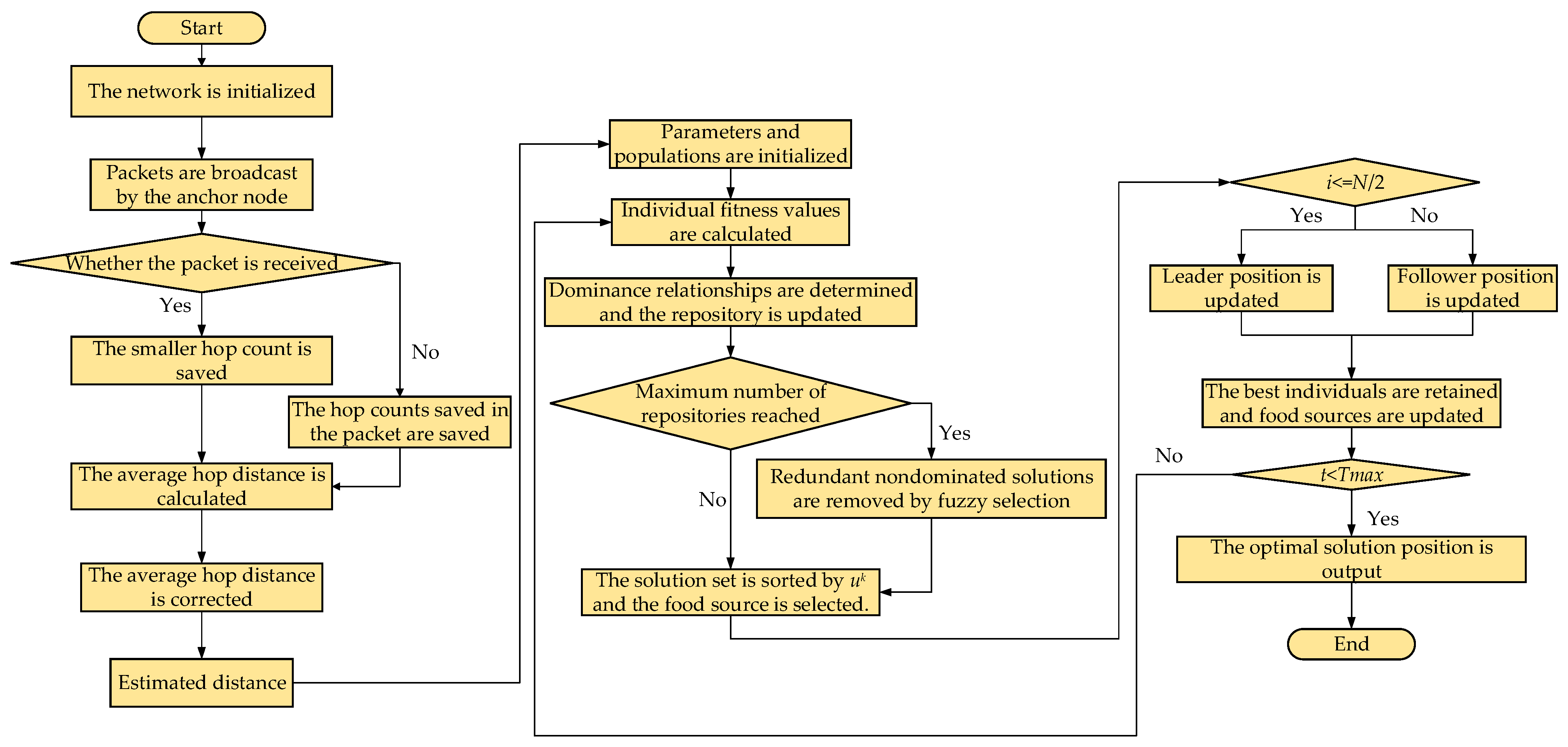
3.6. IMSSA-DV-Hop Algorithm Flow Chart

According to the proposed algorithm improvement strategy, the IMSSA-DV-Hop algorithm is proposed, and the flow chart is shown in Figure 1.

4. Experimental Results and Analysis

4.1. Experimental Environment and Evaluation Criteria

To verify the effectiveness of the IMSSA-DV-Hop algorithm, this algorithm is tested and simulated on MATLAB 2016b on a computer configured with Intel (R) Core (TM) i7-7700HQ CPU @ 2.80 GHz processor (Intel, Santa Clara, CA, USA), 16 GB RAM and Windows 10 operating system. The proposed algorithm is firstly compared with the DV-Hop algorithm in square random topology and C-shaped random topology. The range error line diagram is shown in Figure 2.

As can be seen from Figure 2a,b, the IMSSA-DV-Hop algorithm is significantly improved compared with DV-Hop. Second, to verify the effectiveness of the proposed algorithm, a large number of simulation experiments are conducted with different communication radii, node numbers, beacon node numbers, and areas as constraints. The proposed algorithm is compared with the original DV-Hop algorithm, SSA-DV-Hop algorithm, GWO-DV-Hop algorithm, and ISSA-DV-Hop algorithm. To consider the cost of practical application, specific experimental parameters are shown in

Table 1. Experimental parameter settings.

Parameter	Value
Communication radius (R)	25 m
Nodes	100
Beacon nodes	20
Area	100 × 100 m

.

The normalized relative error equation is used as the index for comparison. The relative error equation after normalization is shown in Equation (47):

$$error={\displaystyle {\sum }_{i=1}^N\sqrt{{(x_0-{\widehat{x}}_0)}^2-{(y_0-{\widehat{y}}_0)}^2}}/(N\times R)$$

(47)

where $(x_0,y_0)$ and $({\widehat{x}}_0,{\widehat{y}}_0)$ are the real and estimated coordinates of the unknown node, and N indicates the number of unknown nodes.

The distribution of nodes in the square random topology and C-shaped random topology is shown in Figure 3a,b.

4.2. The Influence of Communication Radius on Localization Error

In this section, we research the influence of different communication radii on localization error. The node numbers and the beacon node numbers remain the same. At the same time, the communication radius is increased from 20 m to 40 m. The comparison results are shown in Figure 4.

As can be seen from Figure 4a, in the square random topology, the errors of the IMSSA-DV-Hop algorithm are close to those of the GWO-DV-Hop algorithm, when R is small and slightly higher than that of the SSA-DV-Hop algorithm and the ISSA-DV-Hop algorithm. However, with the increase in R, the localization errors decrease significantly. In the C-shaped random topology network, as shown in Figure 4b, the IMSSA-DV-Hop algorithm always has the minimum localization error regardless of the size of R.

The specific experimental data are shown in

Table 2. Localization error in different communication radius in square random topology.

Communication Radius		20	25	30	35	40
Square random topology	DV-Hop	0.4793	0.3504	0.3097	0.2958	0.2849
	GWO-DV-Hop	0.3921	0.2397	0.2116	0.2105	0.2051
	SSA-DV-Hop	0.3673	0.2587	0.2304	0.2417	0.2162
	ISSA-DV-Hop	0.3651	0.2360	0.2109	0.2048	0.2024
	IMSSA-DV-Hop	0.3869	0.2163	0.1773	0.1550	0.1402

and

Table 3. Localization error in different communication radius in C-shaped random topology.

Communication Radius		20	25	30	35	40
C-shaped random topology	DV-Hop	1.5847	1.1970	0.9225	0.7766	0.6467
	GWO-DV-Hop	0.8149	0.5525	0.4484	0.4340	0.3692
	SSA-DV-Hop	0.8335	0.5957	0.4966	0.4423	0.3981
	ISSA-DV-Hop	0.7438	0.5283	0.4402	0.3963	0.3589
	IMSSA-DV-Hop	0.7181	0.5172	0.4311	0.3832	0.3322

. The bolded data in Table are the optimal localization error values.

It can be seen from Table 2 that in square random topology, compared with the DV-Hop algorithm, the IMSSA-DV-Hop algorithm reduces the localization errors by 19.28%, 38.27%, 42.75%, 47.60%, and 50.79%. It can be seen from Table 3 that in the C-shaped random topology, the errors are reduced by 54.69%, 56.79%, 53.27%, 50.66%, and 48.63%. The comparison of localization errors improvement is shown in Figure 5. Compared with the GWO-DV-Hop algorithm, the localization errors of the IMSSA-DV-Hop algorithm in the two topologies are increased by 31.64% and 11.88%.

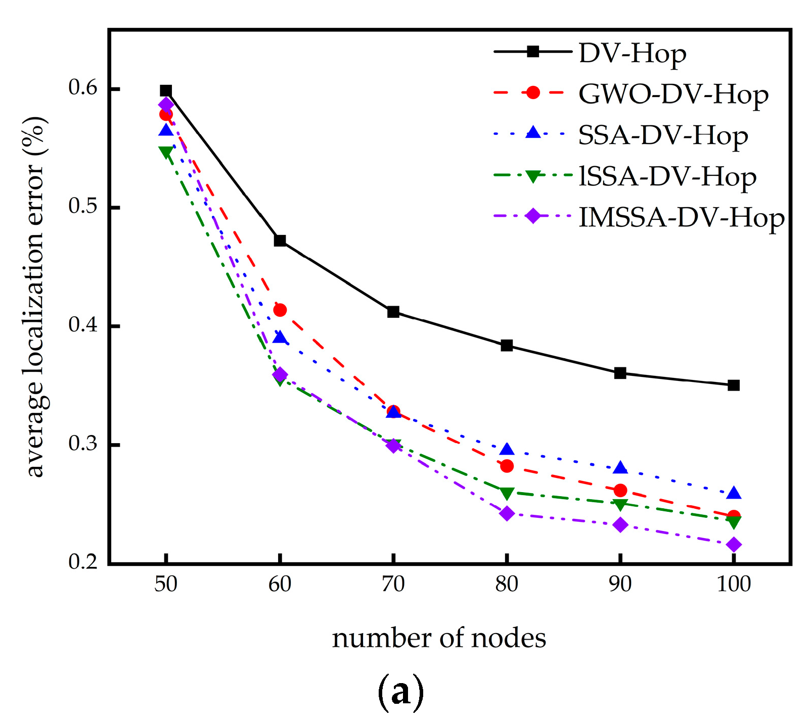
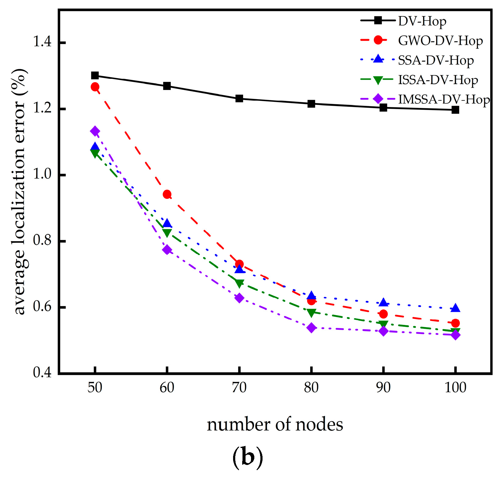
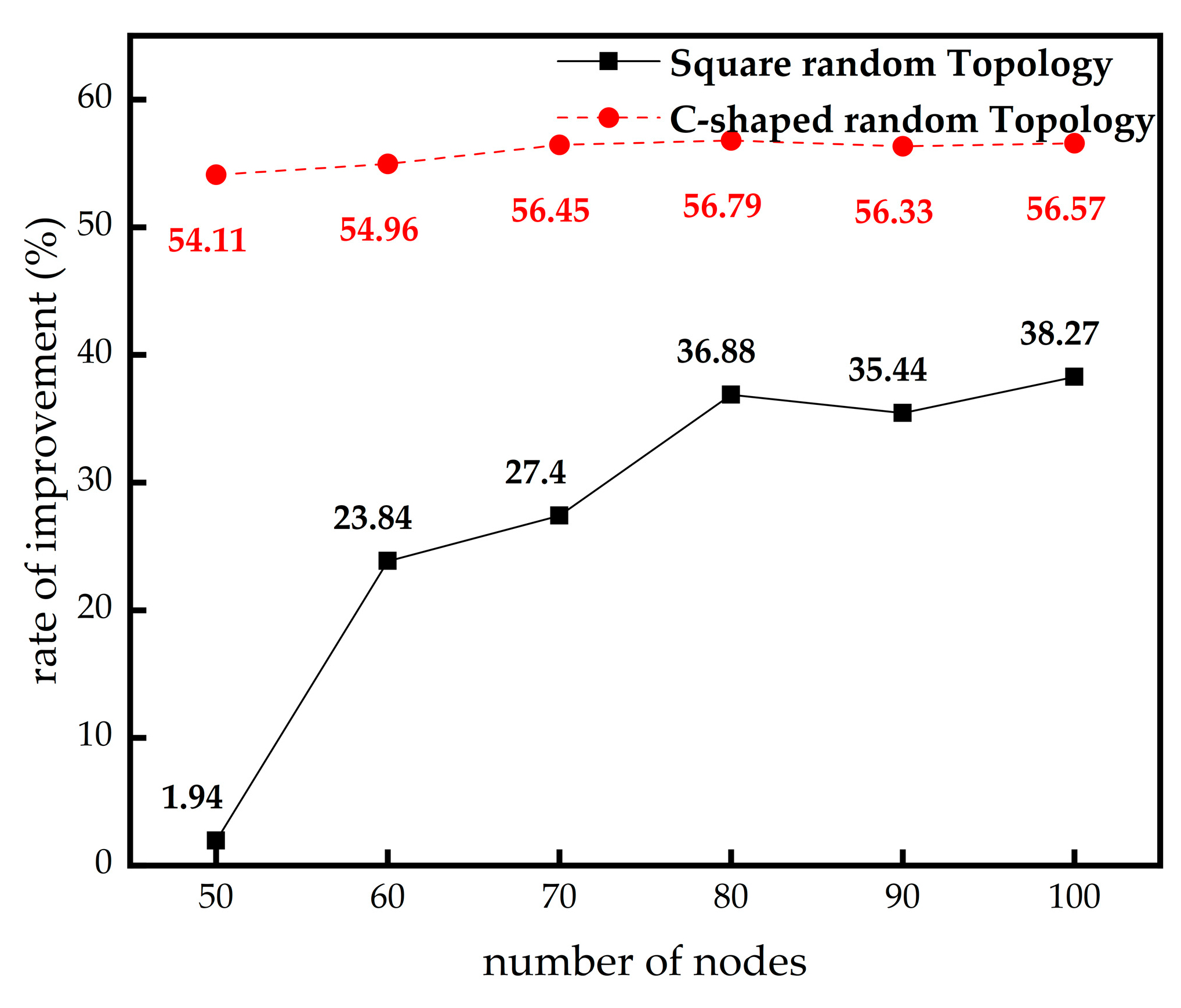
4.3. The Influence of Node Numbers on Localization Error

In this section, we investigate the effect of different node numbers on the localization error. The communication radii and the beacon node numbers remain the same, while the node numbers are increased from 50 to 100. The comparison results are shown in Figure 6.

It can be seen from Figure 6a,b that in the two network topologies, the localization error of the IMSSA-DV-Hop algorithm is slightly greater than that of the three comparison algorithms when the node numbers are small. With the increase in the node numbers, the location errors of the IMSSA-DV-Hop algorithm improve significantly. No matter how the node numbers change, it is better than the DV-Hop algorithm.

The specific experimental data are shown in

Table 4. Localization error in different number of nodes in square random topology.

Number of Nodes		50	60	70	80	90	100
Square random Topology	DV-Hop	0.5986	0.4723	0.4124	0.3839	0.3608	0.3504
	GWO-DV-Hop	0.5789	0.4141	0.3284	0.2824	0.2620	0.2397
	SSA-DV-Hop	0.5644	0.3897	0.3268	0.2954	0.2798	0.2587
	ISSA-DV-Hop	0.5479	0.3562	0.3014	0.2606	0.2511	0.2360
	IMSSA-DV-Hop	0.5870	0.3597	0.2994	0.2423	0.2329	0.2163

and

Table 5. Localization error in different number of nodes in C-shaped random topology.

Number of Nodes		50	60	70	80	90	100
C-shaped random Topology	DV-Hop	1.3009	1.2689	1.2315	1.2156	1.2036	1.1970
	GWO-DV-Hop	1.2668	0.9418	0.7309	0.6203	0.5806	0.5525
	SSA-DV-Hop	1.0839	0.8523	0.7131	0.6338	0.6122	0.5957
	ISSA-DV-Hop	1.0680	0.8284	0.6751	0.5868	0.5509	0.5283
	IMSSA-DV-Hop	1.1330	0.7749	0.6289	0.5389	0.5288	0.5172

. The bolded data in Table are the optimal localization error values.

From Table 4, in the square random topology, compared with the DV-Hop algorithm, the IMSSA-DV-Hop algorithm reduces the localization errors by 1.94%, 23.84%, 27.40%, 36.88%, 35.44%, and 38.27%. From Table 5, In the C-shaped random topology, it reduces 54.11%, 54.96%, 56.45%, 56.79%, 56.33%, and 56.57%. The comparison of localization error improvement is shown in Figure 7.

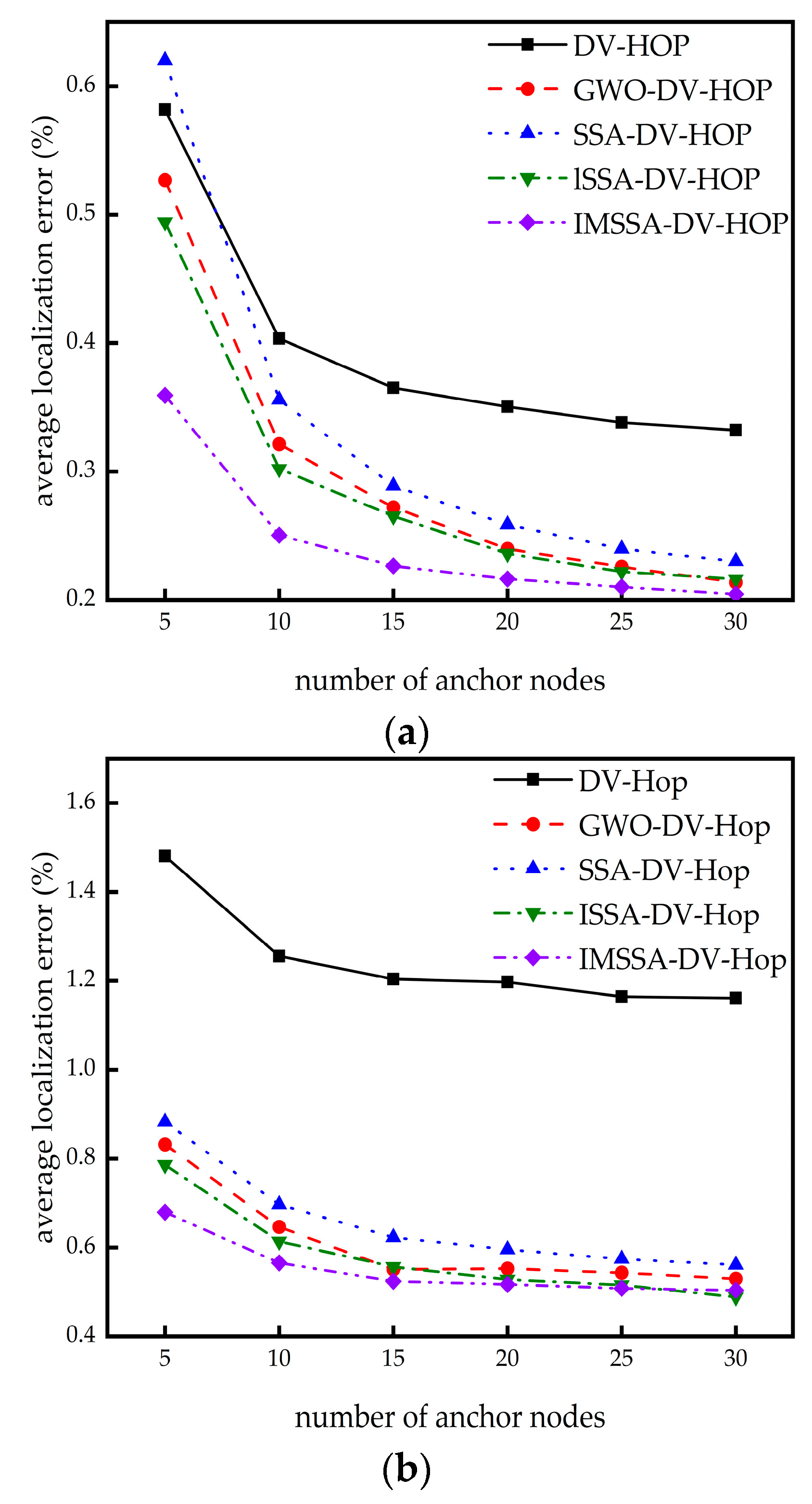
4.4. The Influence of Beacon Node Numbers on Localization Error

In this section, we research the influence of different beacon node numbers on localization error. The node numbers and communication radius remain the same, while the beacon node numbers are increased from 5 to 30. The comparison results are shown in Figure 8.

From Figure 8a,b, it can be seen that the IMSSA-DV-Hop algorithm in two random topologies can achieve lower localization error compared with the three algorithms compared in the case of fewer beacon nodes. In the C-shaped random topology, the performance of this algorithm is close to that of the ISSA-DV-Hop algorithm when the numbers of beacon nodes are large.

The specific experimental data are shown in

Table 6. Localization error in different number of anchor nodes in square random topology.

Number of Beacon Nodes		5	10	15	20	25	30
Square random Topology	DV-Hop	0.5817	0.4035	0.3652	0.3504	0.3382	0.3322
	GWO-DV-Hop	0.5269	0.3213	0.2721	0.2397	0.2258	0.2136
	SSA-DV-Hop	0.6200	0.3559	0.2889	0.2587	0.2397	0.2301
	ISSA-DV-Hop	0.4943	0.3021	0.2652	0.2360	0.2220	0.2162
	IMSSA-DV-Hop	0.3593	0.2504	0.2265	0.2163	0.2101	0.2045

and

Table 7. Localization error in different number of anchor nodes in C-shaped random topology.

Number of Beacon Nodes		5	10	15	20	25	30
C-shaped random Topology	DV-Hop	1.4806	1.2556	1.2038	1.1970	1.1643	1.1610
	GWO-DV-Hop	0.8321	0.6464	0.5507	0.5525	0.5433	0.5298
	SSA-DV-Hop	0.8828	0.6969	0.6229	0.5957	0.5742	0.5611
	ISSA-DV-Hop	0.7864	0.6142	0.5568	0.5283	0.5160	0.4888
	IMSSA-DV-Hop	0.6795	0.5655	0.5242	0.5172	0.5085	0.5042

. The bolded data in Table are the optimal localization error values.

From Table 6, in square random topology, compared with the DV-Hop algorithm, the localization errors of the IMSSA-DV-Hop algorithm are reduced by 38.23%, 37.94%, 37.98%, 38.27%, 37.88%, and 38.44%. From Table 7, In the C-shaped random topology, the localization errors are reduced by 54.11%, 54.96%, 56.45%, 56.79%, 56.33%, and 56.57%. The comparison of localization error improvement is shown in Figure 9. Compared with ISSA-DV-Hop, the localization errors of IMSSA-DV-Hop in the two topologies are increased by 27.31% and 13.59%.

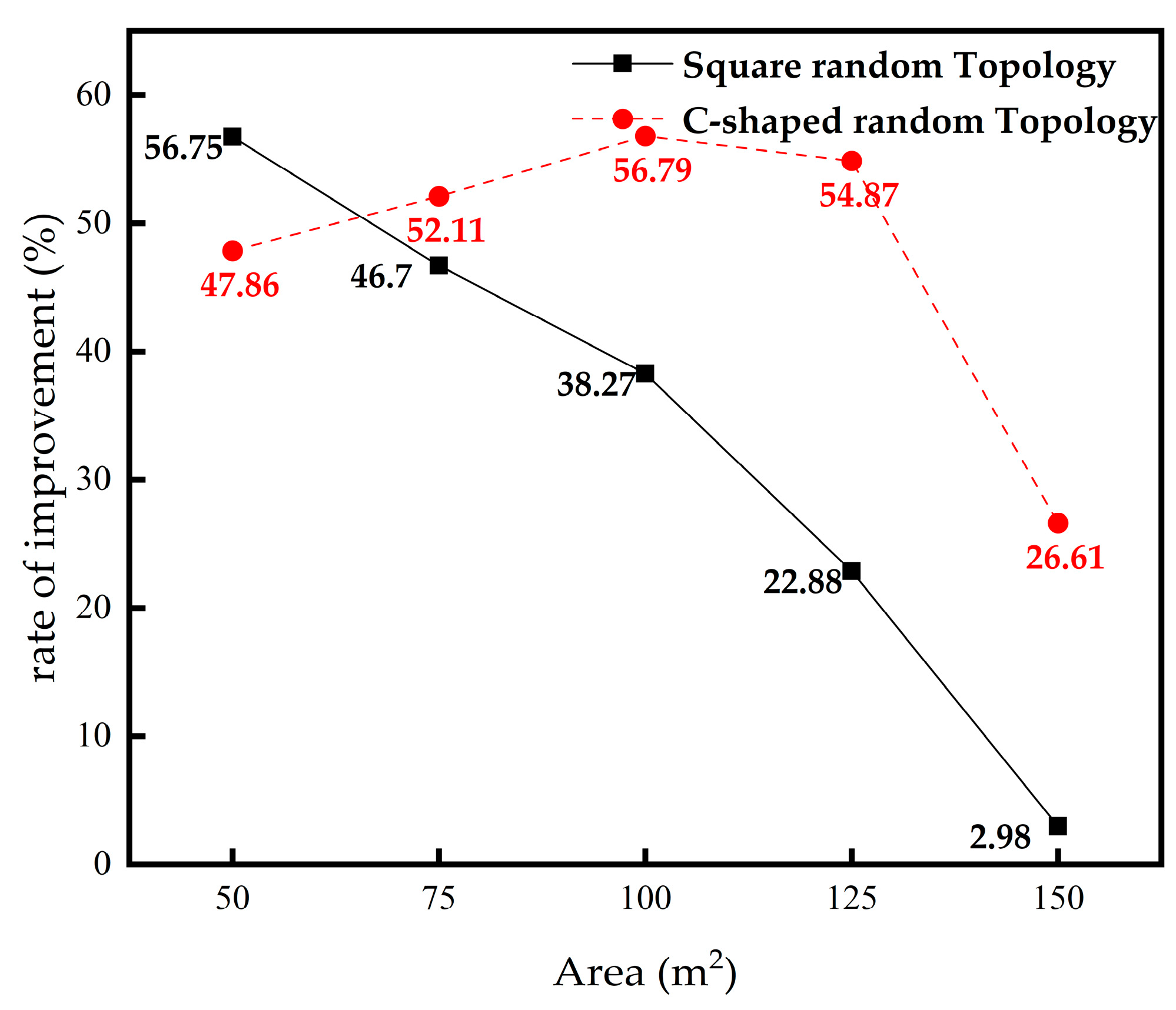
4.5. The Influence of Area on Localization Error

In this section, we study the influence of different regional areas on localization error. The area is increased from 50 × 50 m to 150 × 150 m. The comparison results are shown in Figure 10.

It can be seen from Figure 10a,b that the IMSSA-DV-Hop algorithm is significantly superior to the DV-Hop algorithm and three comparison algorithms in the two random topologies when the area is small at the initial stage. However, in the square topology structure, with the increase in the area, the localization errors of the proposed algorithm and the three comparison algorithms increase significantly. However, in the two topologies, the proposed algorithm is superior to the DV-Hop algorithm regardless of the size of the area.

The specific experimental data are shown in

Table 8. Localization error in different Area in square random topology.

Area		50	75	100	125	150
square random Topology	DV-Hop	0.2833	0.3026	0.3504	0.4813	0.8404
	GWO-DV-Hop	0.2172	0.2139	0.2397	0.3717	1.2178
	SSA-DV-Hop	0.2214	0.2227	0.2587	0.4085	0.9347
	ISSA-DV-Hop	0.1854	0.1730	0.2360	0.3589	0.9519
	IMSSA-DV-Hop	0.1225	0.1613	0.2163	0.3947	1.1674

and

Table 9. Localization error in different Area in C-shaped random topology.

Area		50	75	100	125	150
C-shaped random Topology	DV-Hop	0.5102	0.8216	1.1970	1.5913	1.9785
	GWO-DV-Hop	0.3378	0.4127	0.5525	0.8108	1.4908
	SSA-DV-Hop	0.3569	0.4494	0.5957	0.8523	1.4290
	ISSA-DV-Hop	0.3353	0.4045	0.5283	0.7418	1.4082
	IMSSA-DV-Hop	0.2660	0.3935	0.5172	0.7181	1.4520

. The bolded data in Table are the optimal localization error values.

As can be seen from Table 8, in the square random topology, the localization errors of the IMSSA-DV-Hop algorithm are reduced by 56.75%, 46.70%, 38.27%, 22.88%, and 2.98%, compared with the DV-Hop algorithm. As can be seen from Table 9, localization errors in C-shaped random topology are reduced by 47.86%, 52.11%, 56.79%, 54.87%, and 26.61%. The comparison of localization error improvement is shown in Figure 11.

5. Conclusions

In this paper, we propose an IMSSA-DV-Hop localization algorithm, which uses a multi-objective model based on the DV-Hop single-objective model to reduce the localization error. The first stage of traditional DV-Hop adopts subdivide hop count, average hop distance based, and minimum mean-square error weighting to reduce the errors in the first two stages of the DV-Hop algorithm and improve the localization accuracy. In IMSSA, the initial population of a good point-set is used to facilitate getting rid of local optimal solutions. Additionally, replacing the selection mechanism in the multi-objective salp swarm algorithm with fuzzy selection well selects the desired non-dominated solutions in the repository. In addition, the Levy flight strategy and the floating algorithm position update formula are used in the leader and follower position update, respectively, which improves the search efficiency of the algorithm and reduces the localization error. Experiments are conducted under two network topologies, and the experimental results show that the IMSSA-DV-Hop algorithm outperforms DV-Hop, GWO-DV-Hop, SSA-DV-Hop, and ISSA-DV-Hop.

References

1. Kanwar, V.; Kumar, A. DV-Hop-based range-free localization algorithm for wireless sensor network using runner-root optimization. J. Supercomput. 2020, 77, 3044–3061. [Google Scholar] [CrossRef]
2. Rawat, P.; Singh, K.D.; Chaouchi, H.; Bonnin, J.M. Wireless sensor networks: A survey on recent developments and potential synergies. J. Supercomput. 2013, 68, 1–48. [Google Scholar] [CrossRef]
3. Elhabyan, R.; Shi, W.; St-Hilaire, M. Coverage Protocols for Wireless Sensor Networks: Review and Future Directions. J. Commun. Netw. 2019, 21, 45–60. [Google Scholar] [CrossRef] [Green Version]
4. Ullah, I.; Shen, Y.; Su, X.; Esposito, C.; Choi, C. A Localization Based on Unscented Kalman Filter and Particle Filter Localization Algorithms. IEEE Access 2020, 8, 2233–2246. [Google Scholar] [CrossRef]
5. Wan, X.W.; Lu, J.C. Improved DV-Hop Localization Algorithm Based on Weighted Least Squares Cycle Optimization in Anisotropic Networks. Wirel. Pers. Commun. 2022, 126, 895–909. [Google Scholar] [CrossRef]
6. Messous, S.; Liouane, H. Online Sequential DV-Hop Localization Algorithm for Wireless Sensor Networks. Mob. Inf. Syst. 2020, 2020, 8195309. [Google Scholar] [CrossRef]
7. Ahmad, T.; Li, X.J.; Seet, B.C.; Cano, J.C. Social Network Analysis Based Localization Technique with Clustered Closeness Centrality for 3D Wireless Sensor Networks. Electronics 2020, 9, 738. [Google Scholar] [CrossRef]
8. Chen, T.F.; Hou, S.X.; Sun, L.J.; Sun, K.K. An Enhanced DV-Hop Localization Scheme Based on Weighted Iteration and Optimal Beacon Set. Electronics 2022, 11, 1774. [Google Scholar] [CrossRef]
9. Zhang, L.Z. Improved DV-Hop Algorithm Based on Swarm Intelligence for AI and IoT-Federated Applications in Industry 4.0. Math. Probl. Eng. 2022, 2022, 1194752. [Google Scholar] [CrossRef]
10. Sun, L.J.; Chen, T.F. Difference DV_Distance Localization Algorithm Using Correction Coefficients of Unknown Nodes. Sensors 2018, 18, 2860. [Google Scholar] [CrossRef] [Green Version]
11. Yassin, A.; Nasser, Y.; Awad, M.; Al-Dubai, A.; Liu, R.; Yuen, C.; Raulefs, R.; Aboutanios, E. Recent Advances in Indoor Localization: A Survey on Theoretical Approaches and Applications. IEEE Commun. Surv. Tutor. 2017, 19, 1327–1346. [Google Scholar] [CrossRef] [Green Version]
12. Wang, Y.; Wang, X.D.; Wang, D.M.; Agrawal, D.P. Range-Free Localization Using Expected Hop Progress in Wireless Sensor Networks. IEEE Trans. Parallel Distrib. Syst. 2009, 20, 1540–1552. [Google Scholar] [CrossRef]
13. Chowdhury, T.J.S.; Elkin, C.; Devabhaktuni, V.; Rawat, D.B.; Oluoch, J. Advances on localization techniques for wireless sensor networks: A survey. Comput. Netw. 2016, 110, 284–305. [Google Scholar] [CrossRef]
14. Gui, L.; Zhang, X.; Ding, Q.; Shu, F.; Wei, A. Reference Anchor Selection and Global Optimized Solution for DV-Hop Localization in Wireless Sensor Networks. Wirel. Pers. Commun. 2017, 96, 5995–6005. [Google Scholar] [CrossRef]
15. Elnahrawy, E.; Xiaoyan, L.; Martin, R.P. The limits of localization using signal strength: A comparative study. In Proceedings of the First Annual IEEE Communications Society Conference on Sensor and Ad Hoc Communications and Networks, Santa Clara, CA, USA, 4–7 October 2004; pp. 406–414. [Google Scholar] [CrossRef] [Green Version]
16. Singh, P.; Mittal, N.; Salgotra, R. Comparison of range-based versus range-free WSNs localization using adaptive SSA algorithm. Wirel. Netw. 2022, 28, 1625–1647. [Google Scholar] [CrossRef]
17. Chen, T.F.; Hou, S.X.; Sun, L.J. An Enhanced DV-Hop Positioning Scheme Based on Spring Model and Reliable Beacon Node Set. Comput. Netw. 2022, 209, 108926. [Google Scholar] [CrossRef]
18. Chen, H.Y.; Liu, B.; Huang, P.; Liang, J.L.; Gu, Y. Mobility-Assisted Node Localization Based on TOA Measurements Without Time Synchronization in Wireless Sensor Networks. Mob. Netw. Appl. 2012, 17, 90–99. [Google Scholar] [CrossRef]
19. Luomala, J.; Hakala, I. Analysis and evaluation of adaptive RSSI-based ranging in outdoor wireless sensor networks. Ad Hoc Netw. 2019, 87, 100–112. [Google Scholar] [CrossRef]
20. Mao, G.Q.; Fidan, B.; Anderson, B.D.O. Wireless sensor network localization techniques. Comput. Netw. 2007, 51, 2529–2553. [Google Scholar] [CrossRef] [Green Version]
21. Han, G.; Xu, H.; Duong, T.Q.; Jiang, J.; Hara, T. Localization algorithms of Wireless Sensor Networks: A survey. Telecommun. Syst. 2011, 52, 2419–2436. [Google Scholar] [CrossRef]
22. Liu, J.P.; Liu, M.; Du, X.J.; Stanimirovi, P.S.; Jin, L. An improved DV-Hop algorithm for wireless sensor networks based on neural dynamics. Neurocomputing 2022, 491, 172–185. [Google Scholar] [CrossRef]
23. Jiang, R.; Yang, Z. An improved centroid localization algorithm based on iterative computation for wireless sensor network. Acta Phys. Sin. 2016, 65, 030101. [Google Scholar] [CrossRef]
24. Liu, J.; Wang, Z.; Yao, M.; Qiu, Z. VN-APIT: Virtual nodes-based range-free APIT localization scheme for WSN. Wirel. Netw. 2015, 22, 867–878. [Google Scholar] [CrossRef]
25. Wang, X.; Nie, Y. An improved distance vector-Hop localization algorithm based on coordinate correction. Int. J. Distrib. Sens. Netw. 2017, 13. [Google Scholar] [CrossRef] [Green Version]
26. Niculescu, D.; Nath, B. DV based positioning in ad hoc networks. Telecommun. Syst. 2003, 22, 267–280. [Google Scholar] [CrossRef]
27. Cui, L.; Xu, C.; Li, G.; Ming, Z.; Feng, Y.; Lu, N. A high accurate localization algorithm with DV-Hop and differential evolution for wireless sensor network. Appl. Soft Comput. 2018, 68, 39–52. [Google Scholar] [CrossRef]
28. Messous, S.; Liouane, H.; Cheikhrouhou, O.; Hamam, H. Improved Recursive DV-Hop Localization Algorithm with RSSI Measurement for Wireless Sensor Networks. Sensors 2021, 21, 4152. [Google Scholar] [CrossRef]
29. Zhang, Z.-Y.; Gou, X.; Li, Y.-P.; Shan-shan, H. DV-Hop Based Self-Adaptive Positioning in Wireless Sensor Networks. In Proceedings of the 5th International Conference on Wireless Communications, Networking and Mobile Computing, Beijing, China, 24–26 September 2009. [Google Scholar] [CrossRef]
30. Shoufeng, H.; Xiaojia, Z.; Xinxin, L. A novel DV-Hop localization algorithm for asymmetry distributed wireless sensor networks. In Proceedings of the 2010 3rd International Conference on Computer Science and Information Technology, Chengdu, China, 9–11 July 2010; Volume 4, p. 248. [Google Scholar] [CrossRef] [Green Version]
31. Wang, J.; Hou, A.; Tu, Y.; Yu, H. An Improved DV-Hop Localization Algorithm Based on Selected Anchors. Comput. Mater. Contin. 2020, 65, 977–991. [Google Scholar] [CrossRef]
32. Chen, T.; Sun, L.; Wang, Z.; Wang, Y.; Zhao, Z.; Zhao, P. An enhanced nonlinear iterative localization algorithm for DV_Hop with uniform calculation criterion. Ad Hoc Netw. 2021, 111. [Google Scholar] [CrossRef]
33. Gui, L.; Val, T.; Wei, A.; Dalce, R. Improvement of range-free localization technology by a novel DV-hop protocol in wireless sensor networks. Ad Hoc Netw. 2015, 24, 55–73. [Google Scholar] [CrossRef] [Green Version]
34. Peng, B.; Li, L. An improved localization algorithm based on genetic algorithm in wireless sensor networks. Cogn. Neurodyn. 2015, 9, 249–256. [Google Scholar] [CrossRef] [PubMed] [Green Version]
35. Singh, S.P.; Sharma, S.C. A PSO Based Improved Localization Algorithm for Wireless Sensor Network. Wirel. Pers. Commun. 2017, 98, 487–503. [Google Scholar] [CrossRef]
36. Kaur, A.; Kumar, P.; Gupta, G.P. Nature Inspired Algorithm-Based Improved Variants of DV-Hop Algorithm for Randomly Deployed 2D and 3D Wireless Sensor Networks. Wirel. Pers. Commun. 2018, 101, 567–582. [Google Scholar] [CrossRef]
37. Chai, Q.-W.; Chu, S.-C.; Pan, J.-S.; Hu, P.; Zheng, W.-M. A parallel WOA with two communication strategies applied in DV-Hop localization method. EURASIP J. Wirel. Commun. Netw. 2020, 2020, 50. [Google Scholar] [CrossRef]
38. Li, J.; Gao, M.; Pan, J.-S.; Chu, S.-C. A parallel compact cat swarm optimization and its application in DV-Hop node localization for wireless sensor network. Wirel. Netw. 2021, 27, 2081–2101. [Google Scholar] [CrossRef]
39. Sabahat, E.; Eslaminejad, M.; Ashoormahani, E. A new localization method in internet of things by improving beetle antenna search algorithm. Wirel. Netw. 2022, 28, 1067–1078. [Google Scholar] [CrossRef]
40. Wang, P.; Xue, F.; Li, H.; Cui, Z.; Chen, J. A Multi-Objective DV-Hop Localization Algorithm Based on NSGA-II in Internet of Things. Mathematics 2019, 7, 184. [Google Scholar] [CrossRef] [Green Version]
41. Kanwar, V.; Kumar, A. Range Free Localization for Three Dimensional Wireless Sensor Networks Using Multi Objective Particle Swarm Optimization. Wirel. Pers. Commun. 2020, 117, 901–921. [Google Scholar] [CrossRef]
42. Huang, X.; Han, D.; Weng, T.-H.; Wu, Z.; Han, B.; Wang, J.; Cui, M.; Li, K.-C. A localization algorithm for DV-Hop wireless sensor networks based on manhattan distance. Telecommun. Syst. 2022, 81, 207–224. [Google Scholar] [CrossRef]
43. Mirjalili, S.; Gandomi, A.H.; Mirjalili, S.Z.; Saremi, S.; Faris, H.; Mirjalili, S.M. Salp Swarm Algorithm: A bio-inspired optimizer for engineering design problems. Adv. Eng. Softw. 2017, 114, 163–191. [Google Scholar] [CrossRef]
44. He, G.; Lu, X.L. Good point set and double attractors based-QPSO and application in portfolio with transaction fee and financing cost. Expert Syst. Appl. 2022, 209, 118339. [Google Scholar] [CrossRef]
45. Deepa, R.; Venkataraman, R. Enhancing Whale Optimization Algorithm with Levy Flight for coverage optimization in wireless sensor networks. Comput. Electr. Eng. 2021, 94, 107359. [Google Scholar] [CrossRef]
46. Zervoudakis, K.; Tsafarakis, S. A mayfly optimization algorithm. Comput. Ind. Eng. 2020, 145, 106559. [Google Scholar] [CrossRef]
Figure 1. Flow chart of IMSSA-DV-Hop algorithm.
Sensors 23 03698 g001
Figure 2. Ranging error diagrams: (a) square random topology; (b) C-shaped random topology.
Sensors 23 03698 g002
Figure 3. Node distribution diagrams: (a) square random topology; (b) C-shaped random topology.
Sensors 23 03698 g003
Figure 4. Localization error diagrams for different communication radius: (a) square random topology; (b) C-shaped random topology.
Sensors 23 03698 g004
Figure 5. Comparison of localization error improvement in different communication radius.
Sensors 23 03698 g005
Figure 6. Localization error diagrams for different number of nodes: (a) square random topology; (b) C-shaped random topology.
Sensors 23 03698 g006aSensors 23 03698 g006b
Figure 7. Comparison of localization error improvement in different number of nodes.
Sensors 23 03698 g007
Figure 8. Localization error diagrams for different number of anchor nodes: (a) square random topology; (b) C-shaped random topology.
Sensors 23 03698 g008
Figure 9. Comparison of localization error improvement in different number of anchor nodes.
Sensors 23 03698 g009
Figure 10. Localization error diagrams for different Area: (a) square random topology; (b) C-shaped random topology.
Sensors 23 03698 g010
Figure 11. Comparison of localization error improvement in different Area.
Sensors 23 03698 g011