
Highlighting Shooting Opportunities in Football

Abstract
1. Introduction
2. Materials and Methods
2.1. Data Acquisition
2.2. Procedures
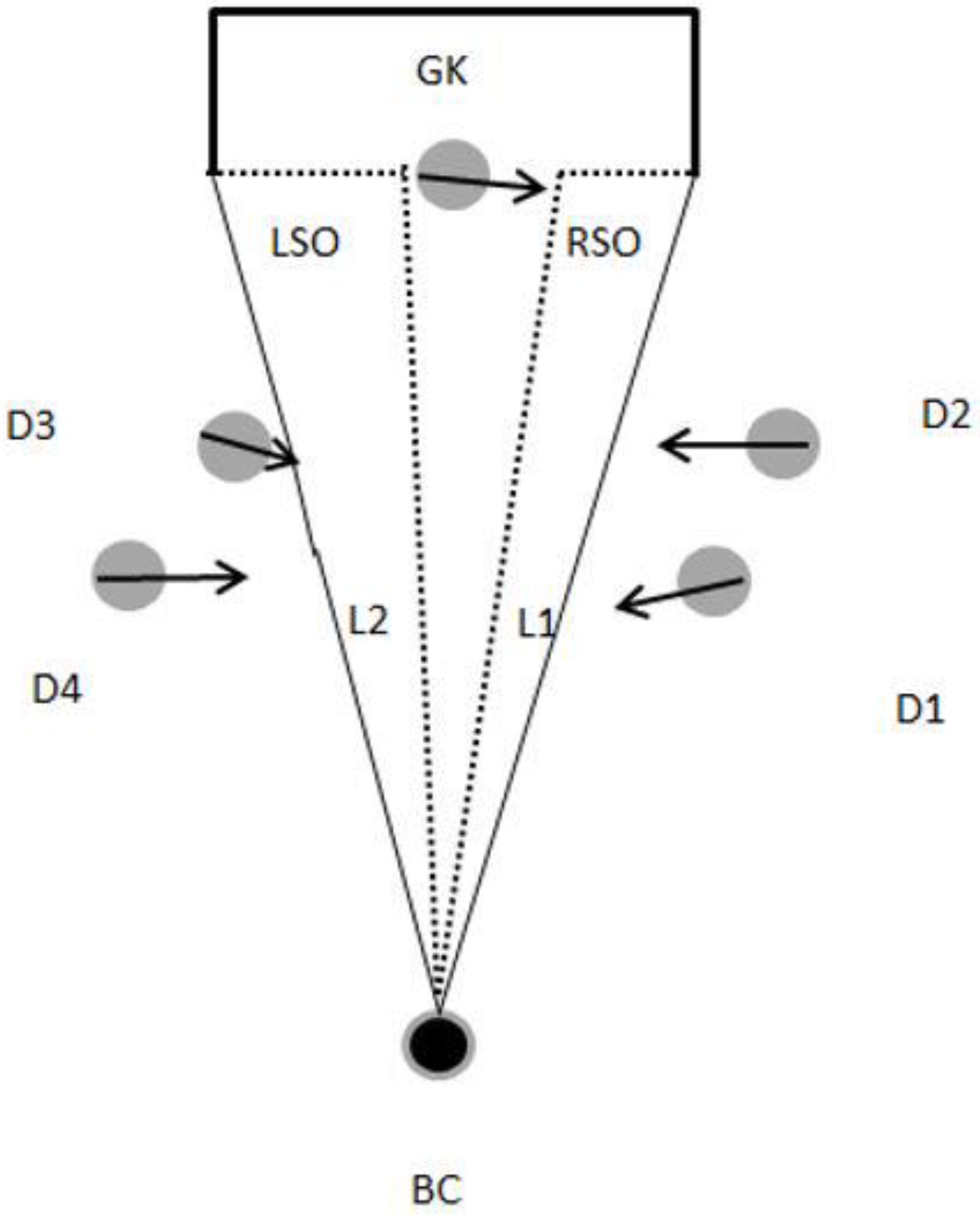
2.3. Algorithm Description
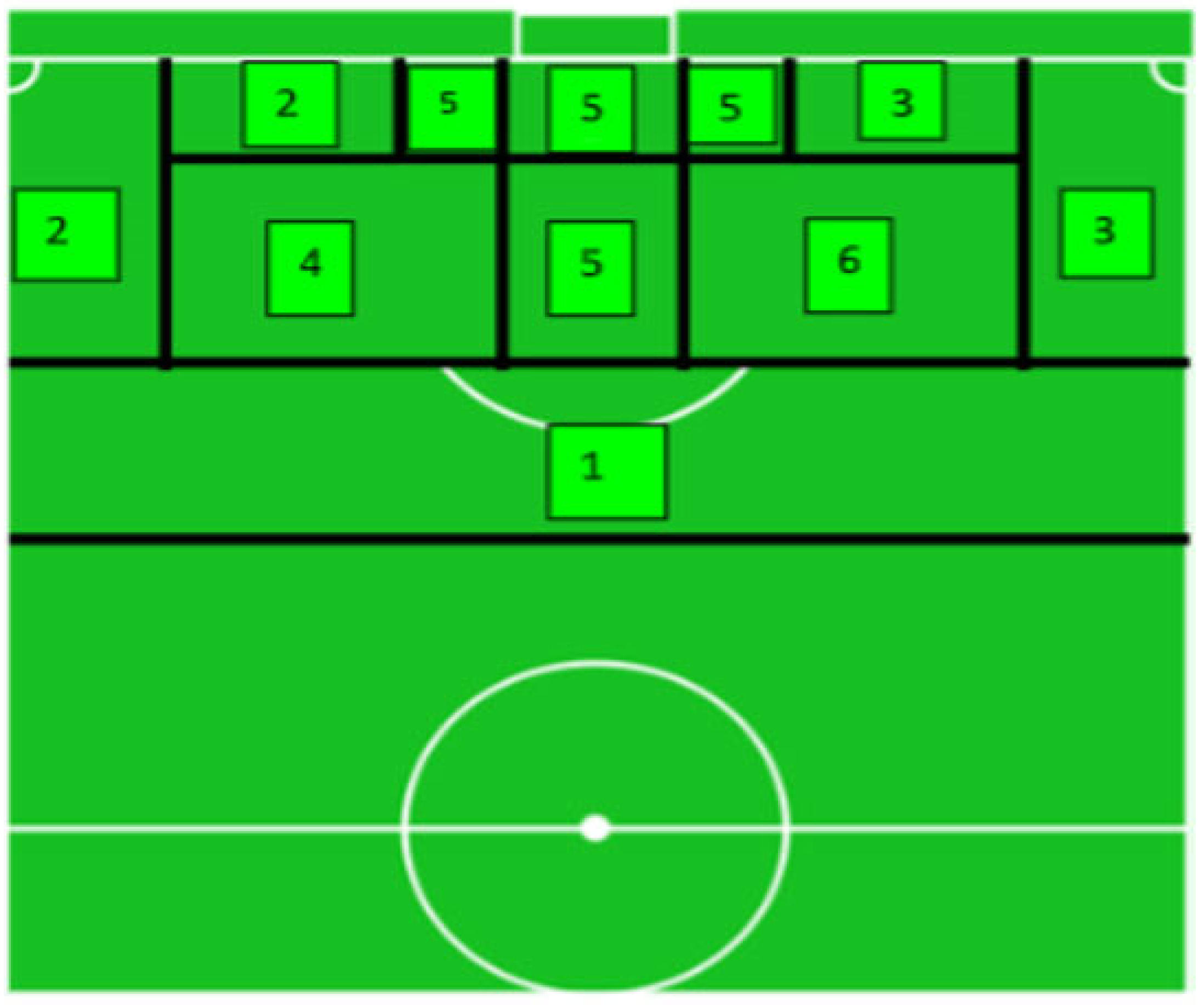
2.4. Distribution of the Shooting Zones and the Level of Threat
2.5. Statistical Procedures
3. Results
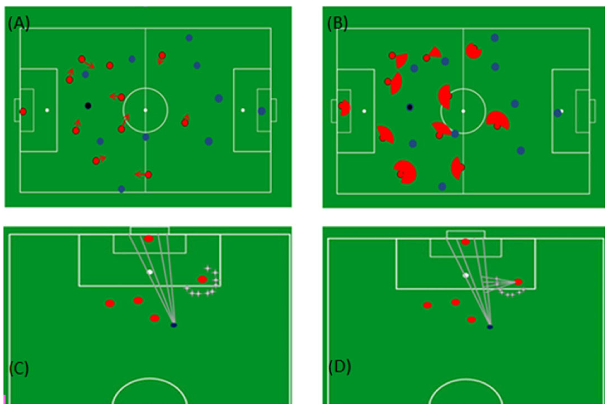
3.1. Landscapes of Shooting Opportunities
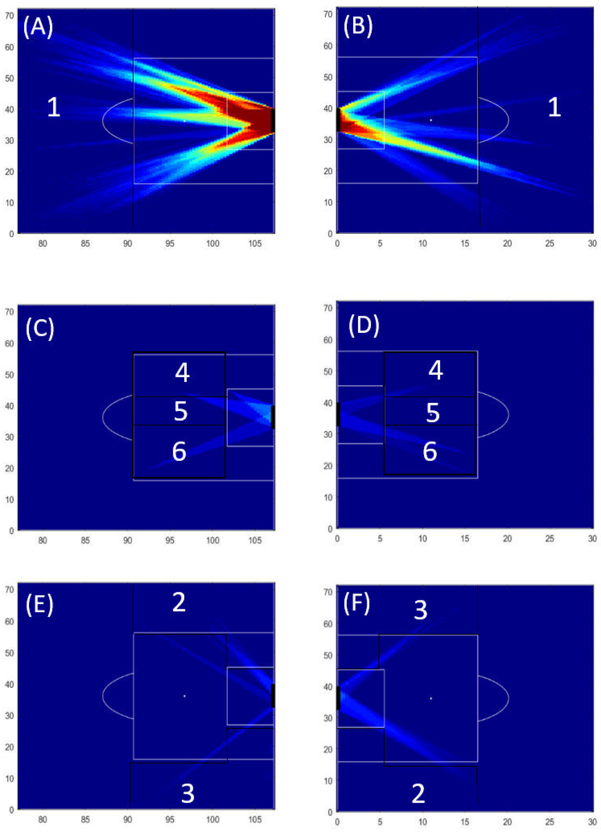
3.1.1. Heatmaps of the Home Team
3.1.2. Heatmaps of the Visitors’ Team
3.2. Descriptive Analysis of Shooting Opportunities
3.3. Statistical Test of Shooting Opportunities
4. Discussion
4.1. Heatmaps and the Threatening Zones
4.2. The Length of the Shooting Opportunities
4.3. Limitations of the Model and Issues for Further Research
5. Conclusions
Author Contributions
Funding
Institutional Review Board Statement
Informed Consent Statement
Data Availability Statement
Acknowledgments
Conflicts of Interest
References
- Gómez-Jordana, L.I.; e Silva, R.A.; Milho, J.; Ric, A.; Passos, P. Illustrating changes in landscapes of passing opportunities along a set of competitive football matches. Sci. Rep. 2021, 11, 9792. [Google Scholar] [CrossRef]
- Passos, P.; E Silva, R.A.; Gomez-Jordana, L.; Davids, K. Developing a two-dimensional landscape model of opportunities for penetrative passing in association football—Stage I. J. Sports Sci. 2020, 38, 2407–2414. [Google Scholar] [CrossRef]
- Rietveld, E.; Kiverstein, J. A rich landscape of affordances. Ecol. Psychol. 2014, 26, 325–352. [Google Scholar] [CrossRef]
- Fajen, B.R.; Riley, M.A.; Turvey, M.T. Information, affordances, and the control of action in sport. Int. J. Sport Psychol. 2009, 40, 79–107. [Google Scholar]
- Gibson, J.J. The Ecological Approach to Visual Perception; Houghton Mifflin: Boston, MA, USA, 1979. [Google Scholar]
- Turvey, M.T. Ecological Foundations of Cognition—Invariants of Perception and Action. In Cognition: Conceptual and Methodological Issues; Pick, H.L., Jr., van den Broek, P.W., Knill, D.C., Eds.; American Psychological Association: Washington, DC, USA, 1992; pp. 85–117. [Google Scholar]
- Duch, J.; Waitzman, J.S.; Amaral, L.A. Quantifying the performance of individual players in a team activity. PLoS ONE 2010, 5, e10937. [Google Scholar] [CrossRef]
- Santos, R.; Passos, P. A Multi-Level Interdependent Hierarchy of Interpersonal Synergies in Team Sports: Theoretical Considerations. Front. Psychol. 2021, 12, 746372. [Google Scholar] [CrossRef]
- Balagué, N.; Pol, R.; Torrents, C.; Ric, A.; Hristovski, R. On the Relatedness and Nestedness of Constraints. Sports Med. Open. 2019, 5, 6. [Google Scholar] [CrossRef]
- Araújo, D.; Passos, P.; Esteves, P.T.; Duarte, R.; Lopes, J.; Hristovski, R.; Davids, K. The micro-macro link in understanding sport tactical behaviours: Integrating information and action at different levels of system analysis in sport. Mov. Sport Sci. 2015, 53–63. [Google Scholar] [CrossRef]
- Kauffman, S. Origins of Order: Self-Organization and Selection in Evolutio; Oxford University Press: Oxford, UK, 1993. [Google Scholar]
- Marsh, K.L.; Richardson, M.J.; Schmidt, R.C. Social connection through joint action and interpersonal coordination. Top. Cogn. Sci. 2009, 1, 320–399. [Google Scholar] [CrossRef]
- Headrick, J.; Davids, K.; Renshaw, I.; Araújo, D.; Passos, P.; Fernandes, O. Proximity-to-goal as a constraint on patterns of behaviour in attacker-defender dyads in team games. J. Sports Sci. 2012, 30, 247–253. [Google Scholar] [CrossRef]
- Laakso, T.; Travassos, B.; Liukkonen, J.; Davids, K. Field location and player roles as constraints on emergent 1-vs-1 interpersonal patterns of play in football. Hum. Mov. Sci. 2017, 54, 347–353. [Google Scholar] [CrossRef]
- Orth, D.; Davids, K.; Araújo, D.; Renshaw, I.; Passos, P.J.M. Effects of a defender on run-up velocity and ball speed when crossing a football. Eur. J. Sport Sci. 2011, 14, S316–S323. [Google Scholar] [CrossRef]
- Passos, P.J.M.; Cordovil, R.; Fernandes, O.D.J.; Barreiros, J. Perceiving affordances in rugby union. J. Sports Sci. 2012, 30, 1175–1182. [Google Scholar] [CrossRef]
- Button, C.; Seifert, L.; Chow, J.Y.; Araujo, D.; Davids, K. Dynamics of Skill Acquisition: An Ecological Dynamics Rationale, 2nd ed.; Human Kinetics: Champaign, IL, USA, 2020. [Google Scholar]
- Davids, K.; Araújo, D.; Hristovski, R.; Passos, P.; Chow, J.Y. Ecological Dynamics and Motor Learning Design in Sport. In Skill Acquisition in Sport: Research, Theory & Practice; Williams, A.M., Hodges, N., Eds.; Routledge: London, UK, 2012; pp. 112–130. [Google Scholar]
- Link, D.; Lang, S.; Seidenschwarz, P. Real Time Quantification of Dangerousity in Football Using Spatiotemporal Tracking Data. PLoS ONE 2016, 11, e0168768. [Google Scholar] [CrossRef]
- Anzer, G.; Bauer, P. A Goal Scoring Probability Model for Shots Based on Synchronized Positional and Event Data in Football (Soccer). Front. Sports Act. Living 2021, 3, 624475. [Google Scholar] [CrossRef]
- Nunome, H.; Lake, M.; Georgakis, A.; Stergioulas, L.K. Impact phase kinematics of instep kicking in soccer. J. Sports Sci. 2006, 24, 11–22. [Google Scholar] [CrossRef]
- Grehaigne, J.F.; Bouthier, D.; David, B. Dynamic-system analysis of opponent relationships in collective actions in soccer. J. Sports Sci. 1997, 15, 137–149. [Google Scholar] [CrossRef]
- Yiannakos, A.; Armatas, V. Evaluation of the goal scoring patterns in European Championship in Portugal 2004. Int. J. Perform. Anal. Sport 2006, 6, 178–188. [Google Scholar] [CrossRef]
- Pollard, R.; Ensum, J.; Taylor, S. Estimating the probability of a shot resulting in a goal: The effects of distance, angle and space. Int. J. Soccer Sci. 2004, 2, 50–55. [Google Scholar]
- Wright, C.; Atkins, S.; Polman, R.; Jones, B.; Sargeson, L. Factors Associated with Goals and Goal Scoring Opportunities in Professional Soccer. Int. J. Perform. Anal. Sport 2011, 11, 438–449. [Google Scholar] [CrossRef]
- Rathke, A. An examination of expected goals and shot efficiency in soccer. J. Hum. Sport Exerc. 2017, 12, S514–S529. [Google Scholar] [CrossRef]
- Schulze, E.; Mendes, B.; Maurício, N.; Furtado, B.; Cesário, N.; Carriço, S.; Meyer, T. Effects of positional variables on shooting outcome in elite football. Sci. Med. Footb. 2018, 2, 93–100. [Google Scholar] [CrossRef]
- Gonzalez-Rodenas, J.; Mitrotasios, M.; Aranda, R.; Armatas, V. Combined effects of tactical, technical and contextual factors on shooting effectiveness in European professional soccer. Int. J. Perform. Anal. Sport 2020, 280–293. [Google Scholar] [CrossRef]
- Krzysztof, M.; Szymanski, D.; Chmura, J. Analysis of goalkeeper performance in the English Premier League. J. Hum. Kinet. 2014, 41, 191–200. [Google Scholar]


| Number of Shooting Opportunities | Mean Time (s) and Standard Deviation (s) | Median Time (s) | Max Time (s) | Min Time (s) | 1st Quartile (s) | 3rd Quartile (s) | IQ Range (s) | |
|---|---|---|---|---|---|---|---|---|
| Home Team | 66 | 1.34 ± 0.78 | 1.2 | 3.6 | 0.4 | 0.6 | 1.8 | 1.2 |
| Visitors’ Team | 9 | 1.6 ± 1.1 | 1 | 3.2 | 0.4 | 0.8 | 2.9 | 2.1 |
| Total | 75 | 1.37 ± 0.82 | 1.2 | 3.6 | 0.4 | 0.6 | 1.8 | 1.2 |
| Zone 1 | Zone 2 | Zone 3 | Zone 4 | Zone 5 | Zone 6 | |
|---|---|---|---|---|---|---|
| Home team | 83% | 3% | 7.5% | 3% | 0% | 3% |
| Visitors’ team | 100% | 0% | 0% | 0% | 0% | 0% |
| Total | 85.3% | 2.6% | 6% | 2.6% | 0% | 2.6% |
| Zone 1 | Zone 2 | Zone 3 | Zone 4 | Zone 5 | Zone 6 | |
|---|---|---|---|---|---|---|
| Home team | 1.4 ± 0.1 | 1.5 ± 0.1 | 0.68 ± 0.13 | 1.3 ± 0.1 | --- | 1.2 ± 0.4 |
| Visitor’s team | 1.6 ± 1.1 | --- | --- | --- | --- | --- |
Disclaimer/Publisher’s Note: The statements, opinions and data contained in all publications are solely those of the individual author(s) and contributor(s) and not of MDPI and/or the editor(s). MDPI and/or the editor(s) disclaim responsibility for any injury to people or property resulting from any ideas, methods, instructions or products referred to in the content. |
© 2023 by the authors. Licensee MDPI, Basel, Switzerland. This article is an open access article distributed under the terms and conditions of the Creative Commons Attribution (CC BY) license (https://creativecommons.org/licenses/by/4.0/).
Share and Cite
Loutfi, I.; Gómez-Jordana, L.I.; Ric, A.; Milho, J.; Passos, P. Highlighting Shooting Opportunities in Football. Sensors 2023, 23, 4244. https://doi.org/10.3390/s23094244
Loutfi I, Gómez-Jordana LI, Ric A, Milho J, Passos P. Highlighting Shooting Opportunities in Football. Sensors. 2023; 23(9):4244. https://doi.org/10.3390/s23094244
Chicago/Turabian StyleLoutfi, Ilias, Luis Ignacio Gómez-Jordana, Angel Ric, João Milho, and Pedro Passos. 2023. "Highlighting Shooting Opportunities in Football" Sensors 23, no. 9: 4244. https://doi.org/10.3390/s23094244
APA StyleLoutfi, I., Gómez-Jordana, L. I., Ric, A., Milho, J., & Passos, P. (2023). Highlighting Shooting Opportunities in Football. Sensors, 23(9), 4244. https://doi.org/10.3390/s23094244