Author Contributions
Conceptualization, H.P.d.S., G.C. and J.F.P.; methodology, C.C., H.P.d.S., D.C.F.S., A.M.M. and G.C.; software, data curation, writing—original draft preparation, and visualization, C.C.; validation, H.P.d.S.; formal analysis, C.C. and H.P.d.S.; investigation, C.C., D.C.F.S. and A.M.M.; writing—review and editing, all authors; supervision, resources and project administration, H.P.d.S., D.C.F.S., A.M.M., G.C. and J.F.P.; funding acquisition, H.P.d.S. All authors have read and agreed to the published version of the manuscript.
Figure 1.
Example of skeletal human body representation: 33 landmarks of MediaPipe Pose, where the right-side landmarks are represented in blue, the left-side landmarks in orange, and the nose landmark in white.
Figure 1.
Example of skeletal human body representation: 33 landmarks of MediaPipe Pose, where the right-side landmarks are represented in blue, the left-side landmarks in orange, and the nose landmark in white.
Figure 2.
Classification of 2D camera-based models for Human Pose Estimation (HPE).
Figure 2.
Classification of 2D camera-based models for Human Pose Estimation (HPE).
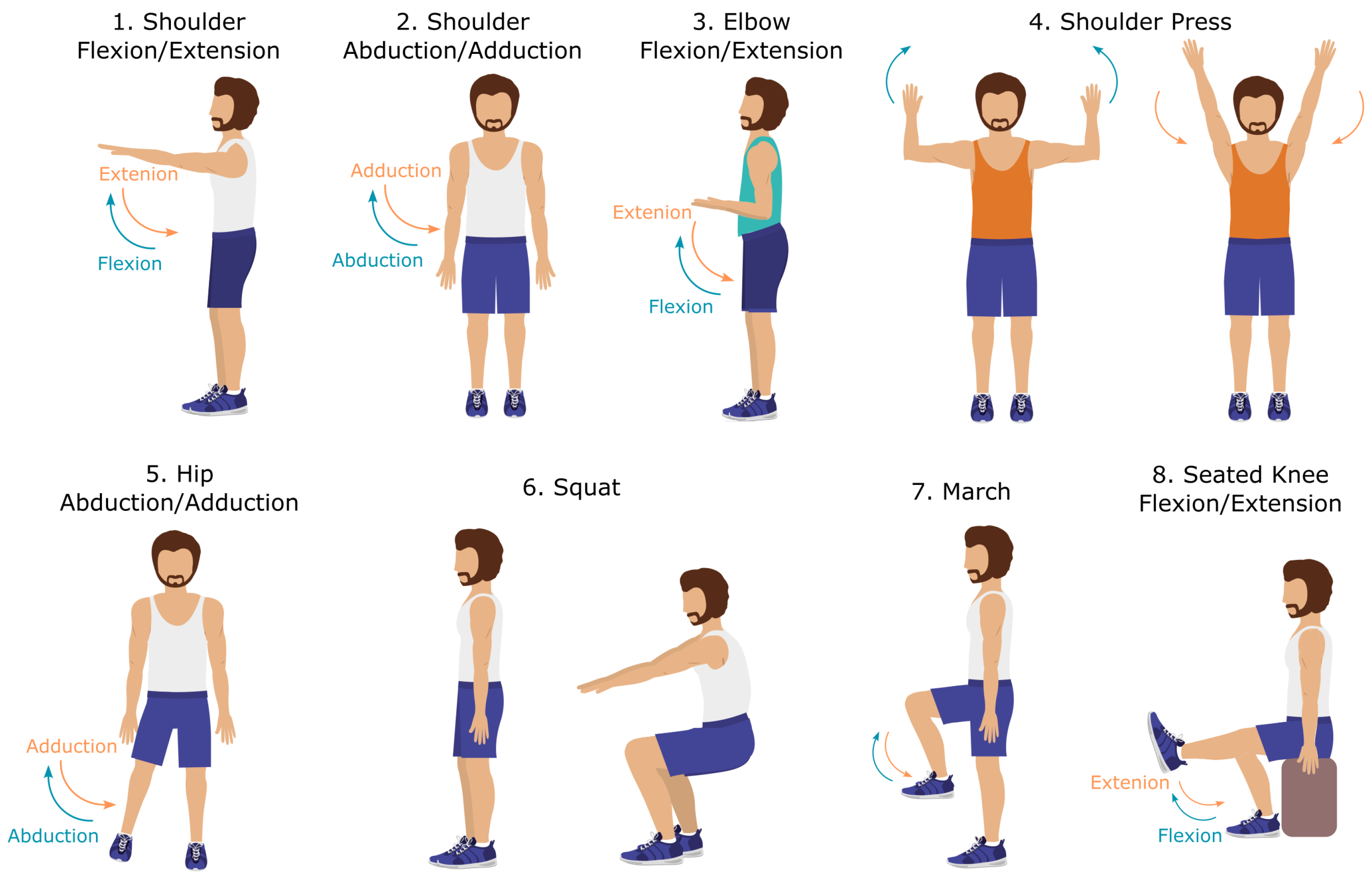
Figure 3.
Eight exercises selected for the experimental study: Shoulder Flexion/Extension (SF), Shoulder Abduction/Adduction (SA), Elbow Flexion/Extension (EF), Shoulder Press (SP), Hip Abduction/Adduction (HA), Squat (SQ), March (MCH), and Seated Knee Flexion/Extension (SKF). Shoulder press and squat exercises are illustrated by a sequence of two representative images of the movement.
Figure 4.
Experimental setup for the data acquisition, showing some of the Qualisys cameras, two 2D cameras, and the relative position between the subject and the two 2D cameras.
Figure 4.
Experimental setup for the data acquisition, showing some of the Qualisys cameras, two 2D cameras, and the relative position between the subject and the two 2D cameras.
Figure 5.
Anatomical location of the six Qualisys MoCap markers.
Figure 5.
Anatomical location of the six Qualisys MoCap markers.
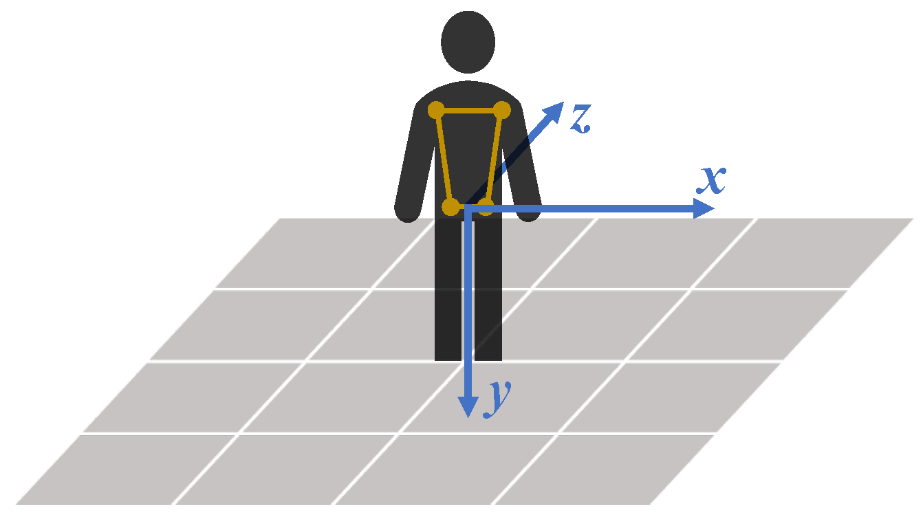
Figure 6.
The 3D Cartesian coordinate system of Qualisys (in orange) and its spatial relation with respect to the participant position during data acquisition.
Figure 6.
The 3D Cartesian coordinate system of Qualisys (in orange) and its spatial relation with respect to the participant position during data acquisition.
Figure 7.
Comparison of the normal vectors of the anatomical planes (in black) with the Qualisys coordinate system (in orange).
Figure 7.
Comparison of the normal vectors of the anatomical planes (in black) with the Qualisys coordinate system (in orange).
Figure 8.
Relation between the participant position and the Cartesian coordinate system of the MediaPipe Pose model for three camera orientations: (a) camera plane parallel to participant frontal plane; (b) camera plane rotated around the Y-axis relative to participant frontal plane; and (c) camera plane rotated around the X-axis relative to participant frontal plane. The camera 2D coordinate system is represented by the X’-axis and Y’-axis, which are parallel to the X-axis and Y-axis of the algorithm coordinate system, respectively.
Figure 9.
The virtual 3D coordinate system of MediaPipe Pose coincident with the normal vectors of the anatomical planes. The origin is the midpoint between the hips. The X-axis is the sagittal plane normal, the Y-axis is the transverse plane normal, and the Z-axis is the frontal plane normal. The four points (representing the shoulders and hips) are used to define the virtual 3D coordinate system.
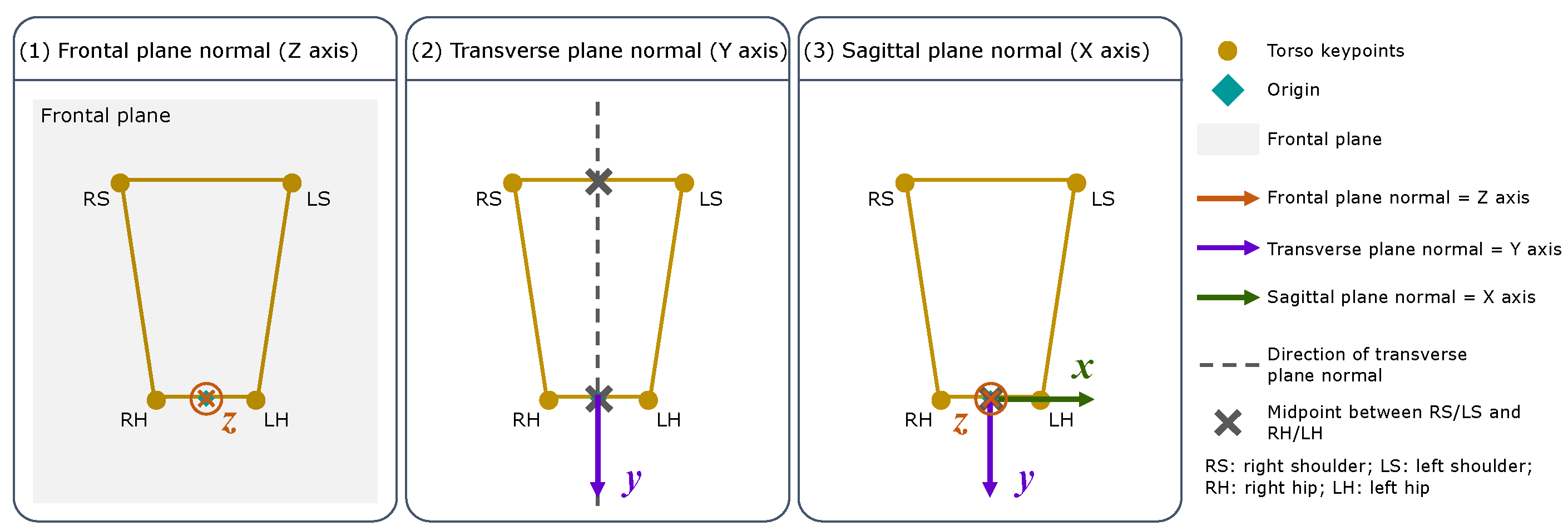
Figure 10.
Representation of virtual 3D coordinate system definition: (1) Z-axis or frontal plane normal; (2) Y-axis or transverse plane normal; and (3) X-axis or sagittal plane normal.
Figure 10.
Representation of virtual 3D coordinate system definition: (1) Z-axis or frontal plane normal; (2) Y-axis or transverse plane normal; and (3) X-axis or sagittal plane normal.
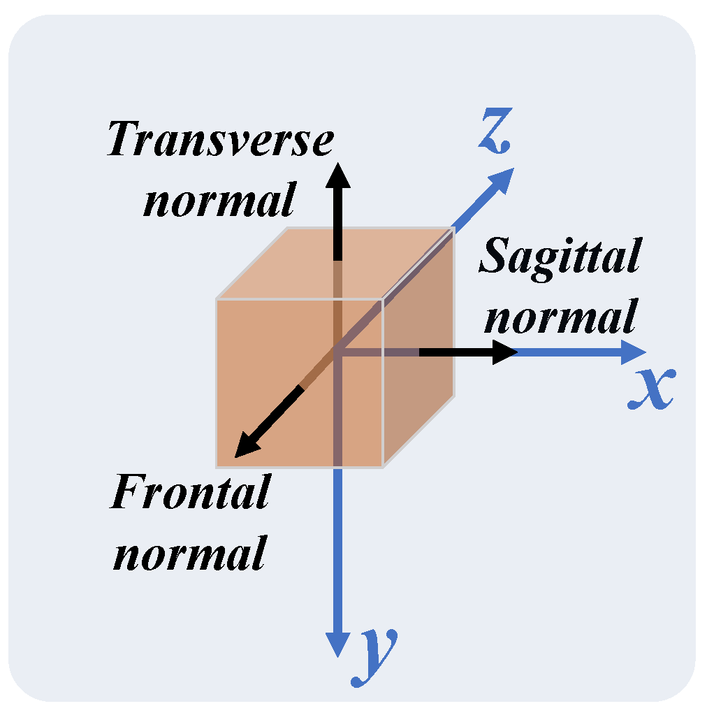
Figure 11.
Comparison of the normal vectors of the anatomical planes (in black) with the MediaPipe Pose virtual coordinate system (in blue).
Figure 11.
Comparison of the normal vectors of the anatomical planes (in black) with the MediaPipe Pose virtual coordinate system (in blue).
Figure 12.
Amplitude calculation between the projected body segment vector and a reference direction.
Figure 12.
Amplitude calculation between the projected body segment vector and a reference direction.
Figure 13.
Data alignment between the Qualisys ground truth amplitudes (in orange) and MediaPipe Pose predicted amplitudes (in blue).
Figure 13.
Data alignment between the Qualisys ground truth amplitudes (in orange) and MediaPipe Pose predicted amplitudes (in blue).
Figure 14.
Example of Qualisys ground truth (in orange) and MediaPipe Pose predicted (in blue) amplitudes for Subject 1 performing SA exercise and SKF exercise. (a,b) show the raw amplitude before the alignment procedure, and (c,d) the aligned amplitude data, before segmenting the sample to extract the exercise repetitions.
Figure 15.
Relation between Qualisys and MediaPipe Pose motion amplitudes for (a) SA exercise and (b) SKF exercise. Each color represents a different subject, and the yellow line is the linear regression that best fits the amplitude data for the exercise; the coefficient of determination () and the linear regression equation (slope and intercept) are also shown, where y and x are the Qualisys and MediaPipe Pose amplitudes, respectively.
Table 1.
Exercises commonly performed in musculoskeletal physiotherapy sessions, and description of the limb in motion, the plane of movement, and the evaluated joint.
Table 1.
Exercises commonly performed in musculoskeletal physiotherapy sessions, and description of the limb in motion, the plane of movement, and the evaluated joint.
| Exercises | Limb in Motion | Plane of Movement | Evaluated Joint |
|---|
| 1. Shoulder Flexion/Extension (SF) | Right arm | Sagittal | Right shoulder |
| 2. Shoulder Abduction/Adduction (SA) | Right arm | Frontal | Right shoulder |
| 3. Elbow Flexion/Extension (EF) | Arms (bilateral) | Sagittal | Right elbow |
| 4. Shoulder Press (SP) | Arms (bilateral) | Frontal | Right shoulder |
| 5. Hip Abduction/Adduction (HA) | Right leg | Frontal | Right hip |
| 6. Squat (SQ) | Legs (bilateral) | Sagittal | Right knee |
| 7. March (MCH) | Legs (bilateral) | Sagittal | Right hip |
| 8. Seated Knee Flexion/Extension (SKF) | Right leg | Sagittal | Right knee |
Table 2.
Relation between the anatomical location of the six Qualisys MoCap markers and the human joints.
Table 2.
Relation between the anatomical location of the six Qualisys MoCap markers and the human joints.
| MoCap Anatomical Location | Joint |
|---|
| 1. Acromion | Shoulder |
| 2. Lateral epicondyle of humerus | Elbow |
| 3. Styloid apophysis of radius | Wrist |
| 4. Greater trochanter | Hip |
| 5. Lateral epicondyle of the femur | Knee |
| 6. Lateral malleolus of the ankle | Ankle |
Table 3.
Information for the ROM evaluation: plane of movement in which the exercise occurs, the body segment, and the reference direction. ↓ represents vertically downward direction.
Table 3.
Information for the ROM evaluation: plane of movement in which the exercise occurs, the body segment, and the reference direction. ↓ represents vertically downward direction.
| Exercises | Plane of Movement | Body Segment (Joint 1–Joint 2) | Reference Direction |
|---|
| 1. SF | Sagittal | Shoulder–elbow | ↓ |
| 2. SA | Frontal | Shoulder–elbow | ↓ |
| 3. EF | Sagittal | Elbow–wrist | ↓ |
| 4. SP | Frontal | Shoulder–elbow | ↓ |
| 5. HA | Frontal | Hip–knee | ↓ |
| 6. SQ | Sagittal | Knee–hip | Foot-knee |
| 7. MCH | Sagittal | Hip–knee | ↓ |
| 8. SKF | Sagittal | Knee–foot | ↓ |
Table 4.
MAE, in degrees, and MAPE, in percentage, between Qualisys and MediaPipe Pose amplitudes (peak and motion) for each exercise. MAPE color code [
34]: <10% (highly accurate forecast) in green; 10–20% (good forecast) in yellow; 20–50% (reasonable forecast) in light orange; >50% (inaccurate forecast) in dark orange. (s) and (f) indicate sagittal and frontal plane exercises, respectively.
| Exercise | Peak Amplitudes | Motion Amplitudes
(Threshold = 1°) |
|---|
| MAE (°) | MAPE (%) | MAE (°) | MAPE (%) |
|---|
| 1. SF (s) | 28.8 | 28.7 | 15.6 | 66.60 |
| 2. SA (f) | 13.0 | 10.2 | 7.7 | 14.90 |
| 3. EF (s) | 11.7 | 9.6 | 10.6 | 24.2 |
| 4. SP (f) | 13.8 | 9.5 | 18.7 | 23.0 |
| 5. HA (f) | 3.7 | 9.0 | 3.2 | 62.9 |
| 6. SQ (s) | 7.6 | 7.9 | 8.3 | 25.0 |
| 7. MCH (s) | 6.3 | 7.7 | 6.3 | 107.4 |
| 8. SKF (s) | 4.9 | 6.6 | 9.9 | 78.10 |
Table 5.
Correlation analysis between the Qualysis and MediaPipe Pose amplitudes (peak and motion) for each exercise: Pearson correlation coefficient (r) and cosine similarity coefficient (cos_sim). The p-value was <0.001, indicating a statistically significant Pearson coefficient. Color code: >0.9 in green; 0.8–0.9 in yellow; 0.7–0.8 in light orange. (s) and (f) indicate sagittal and frontal plane exercises, respectively.
| Exercise | Peak Amplitudes | Motion Amplitudes |
|---|
| cos_sim | | cos_sim |
|---|
| 1. SF (s) | 0.894 | 0.992 | 0.904 | 0.949 |
| 2. SA (f) | 0.939 | 0.999 | 0.996 | 0.999 |
| 3. EF (s) | 0.903 | 0.997 | 0.963 | 0.990 |
| 4. SP (f) | 0.744 | 0.999 | 0.985 | 0.997 |
| 5. HA (f) | 0.915 | 0.995 | 0.985 | 0.987 |
| 6. SQ (s) | 0.833 | 0.998 | 0.981 | 0.993 |
| 7. MCH (s) | 0.961 | 0.996 | 0.964 | 0.979 |
| 8. SKF (s) | 0.765 | 0.997 | 0.942 | 0.961 |
Table 6.
Linear regression between motion amplitudes of Qualisys and MediaPipe Pose for each exercise: slope and intercept values for the equation that better fits the transformation of predictions (MediaPipe Pose points) into expected data (Qualisys points), coefficient of determination (), and curve shape. (s) and (f) indicate sagittal and frontal plane exercises, respectively.
| Exercise | Motion Amplitudes |
|---|
| Slope | Intercept | | Curve Shape |
|---|
| 1. SF (s) | 0.75 | 11.3 | 0.82 | Not linear |
| 2. SA (f) | 0.89 | 1.72 | 0.99 | Linear |
| 3. EF (s) | 1.23 | −11.86 | 0.93 | Not linear |
| 4. SP (f) | 0.96 | −14.2 | 0.97 | Linear |
| 5. HA (f) | 0.92 | 3.39 | 0.97 | Linear |
| 6. SQ (s) | 1.05 | 5.12 | 0.96 | Linear |
| 7. MCH (s) | 1.03 | −0.82 | 0.93 | Linear |
| 8. SKF (s) | 1.13 | −4.19 | 0.89 | Not linear |


 ,
, 


