Quality Analysis of 3D Point Cloud Using Low-Cost Spherical Camera for Underpass Mapping


Abstract
:1. Introduction
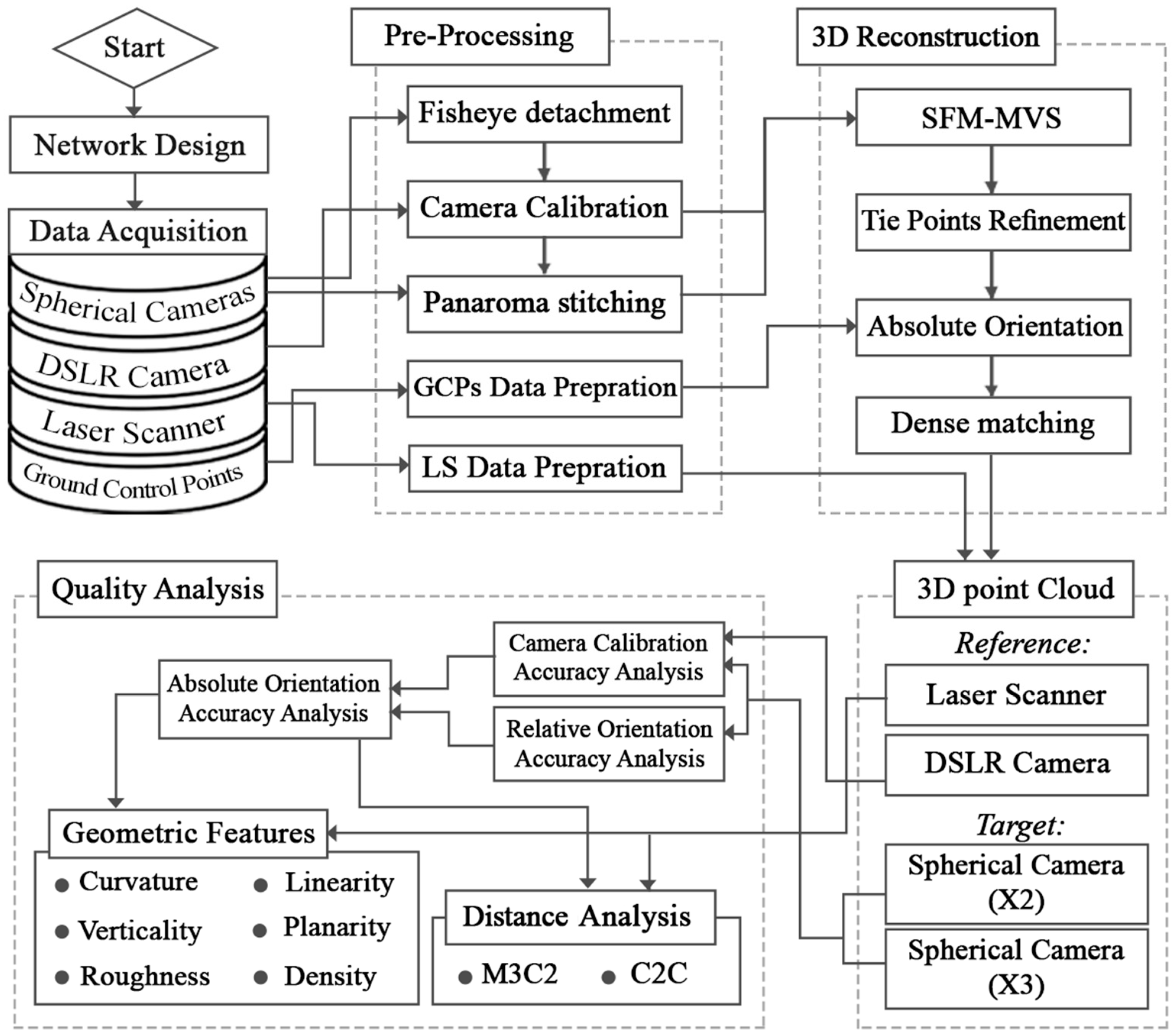
2. Materials and Methods
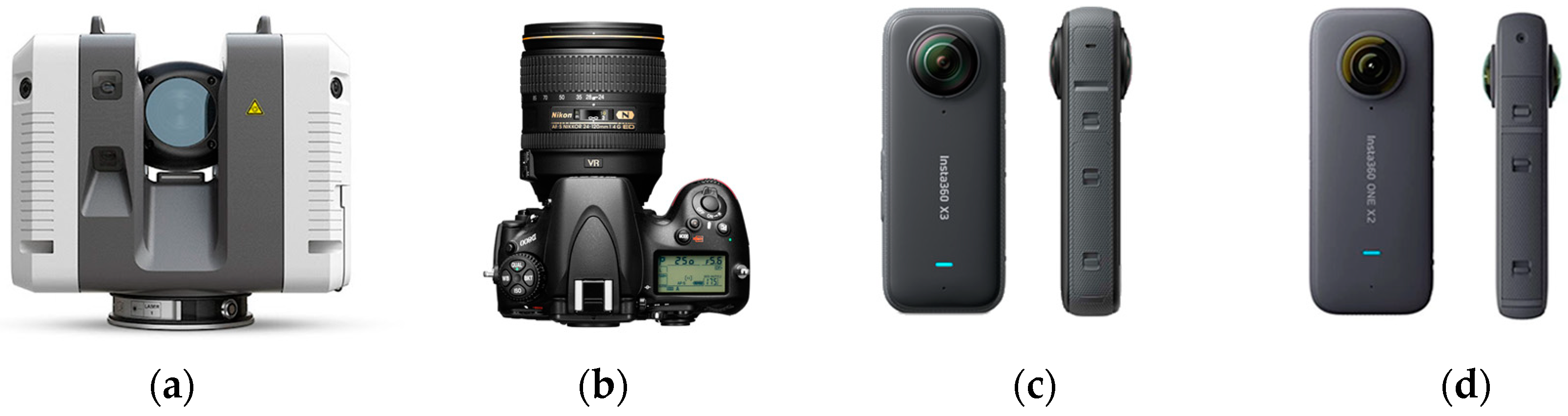
2.1. Case Study and Sensor Selection
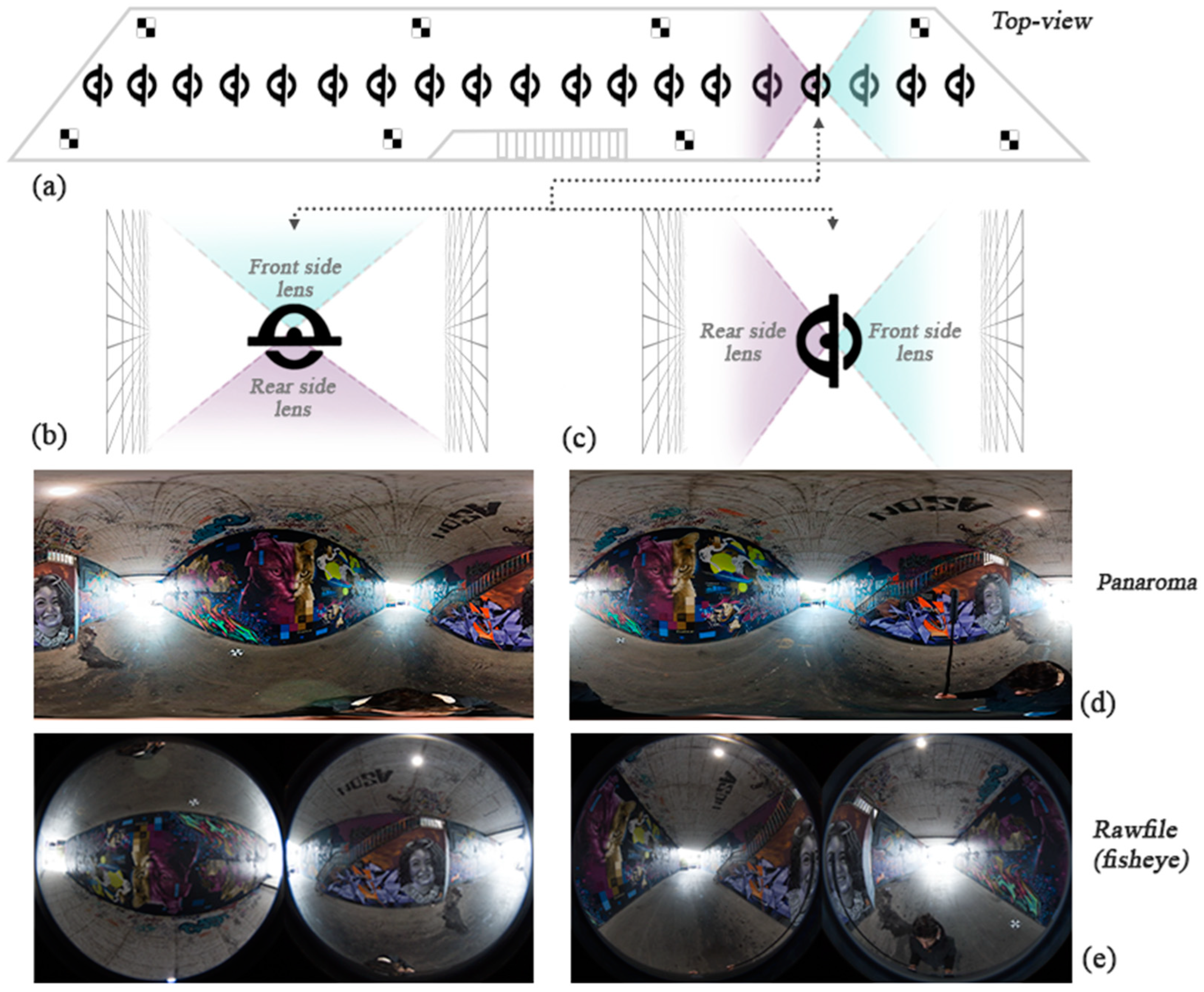
2.2. Network Design
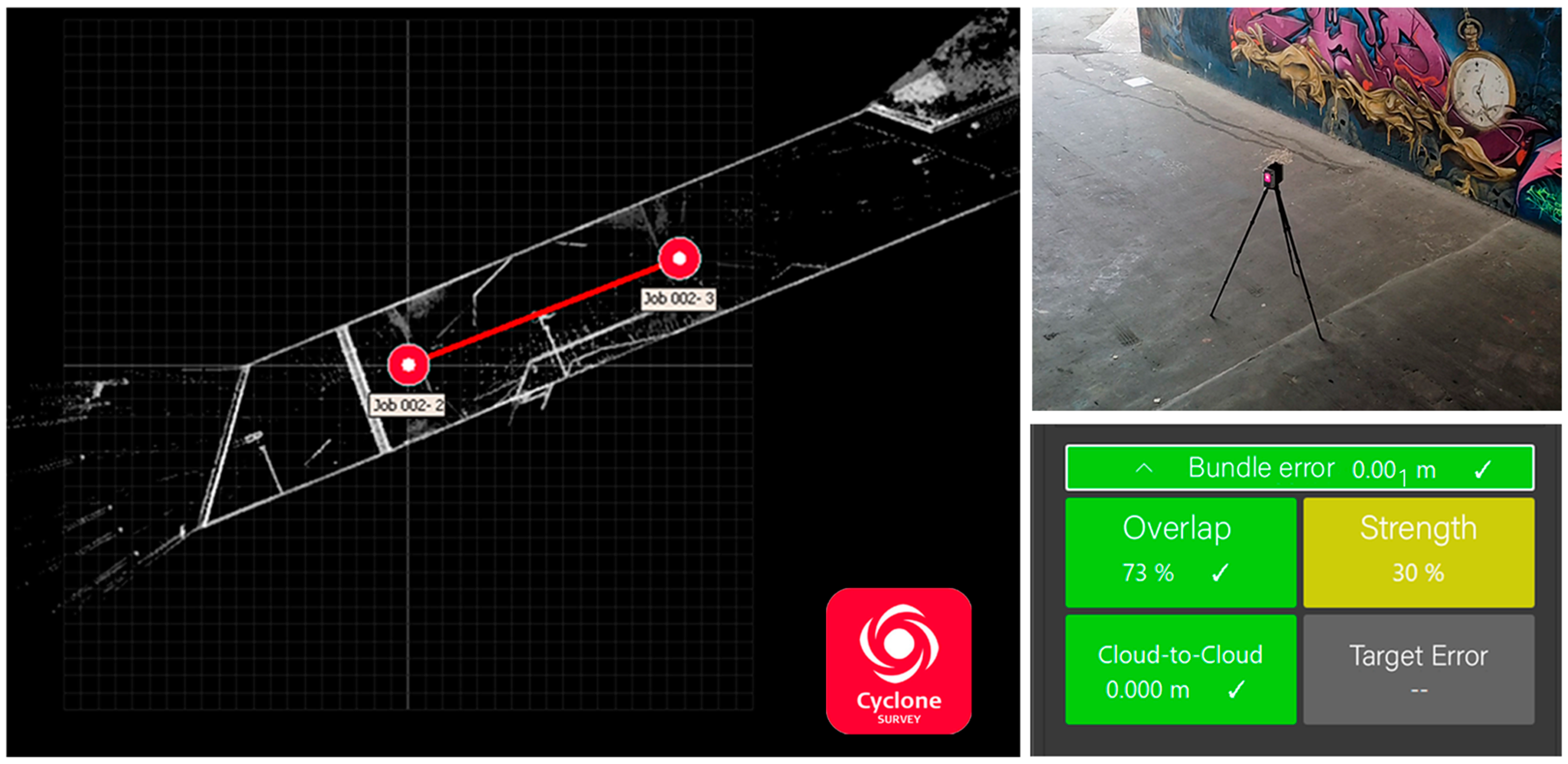
2.3. Data Acquisition
2.4. Pre-Processing
2.4.1. Data Organization
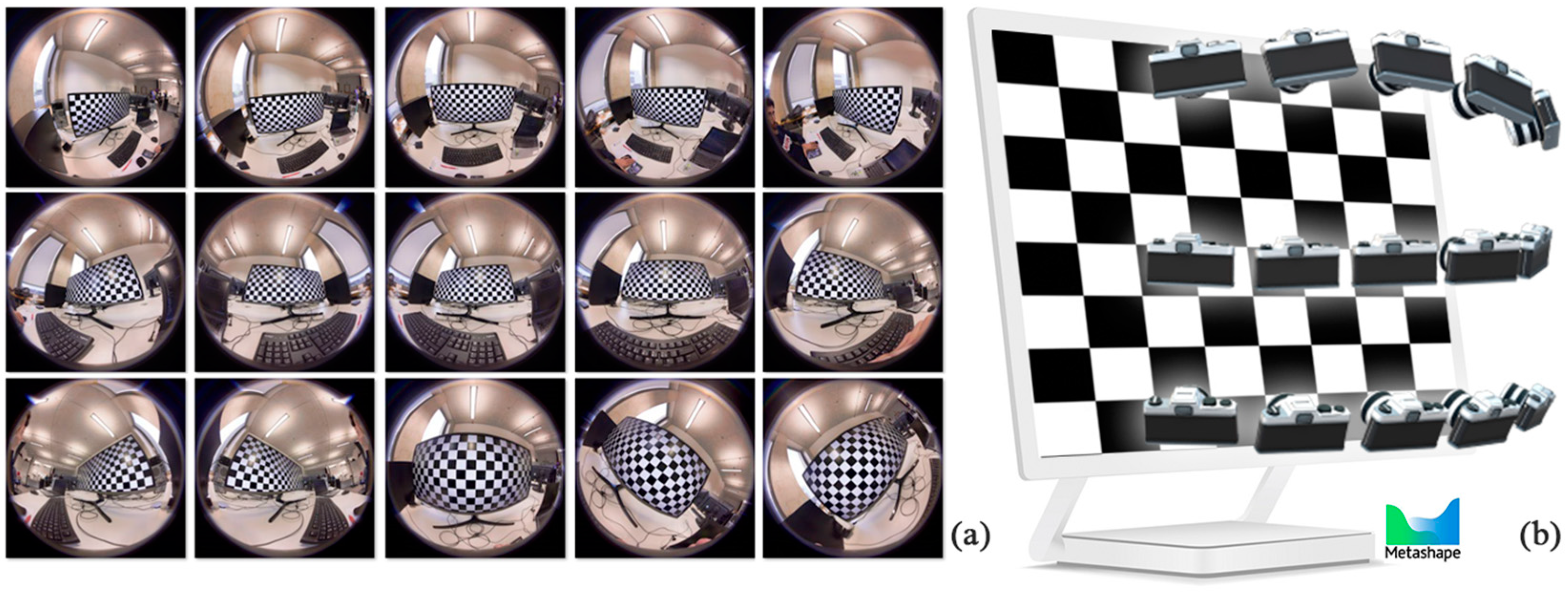
2.4.2. Camera Calibration
2.5. 3D Reconstruction
2.5.1. SFM-MVS
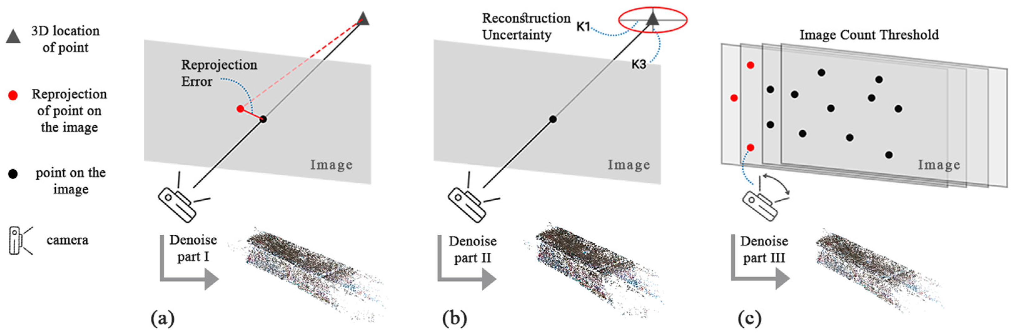
2.5.2. Tie Point Refinement
2.5.3. Absolute Orientation
2.5.4. Dense Matching
2.6. Quality Analysis
2.6.1. Camera Calibration Accuracy Analysis
2.6.2. Relative and Absolute Orientation Accuracy Analysis
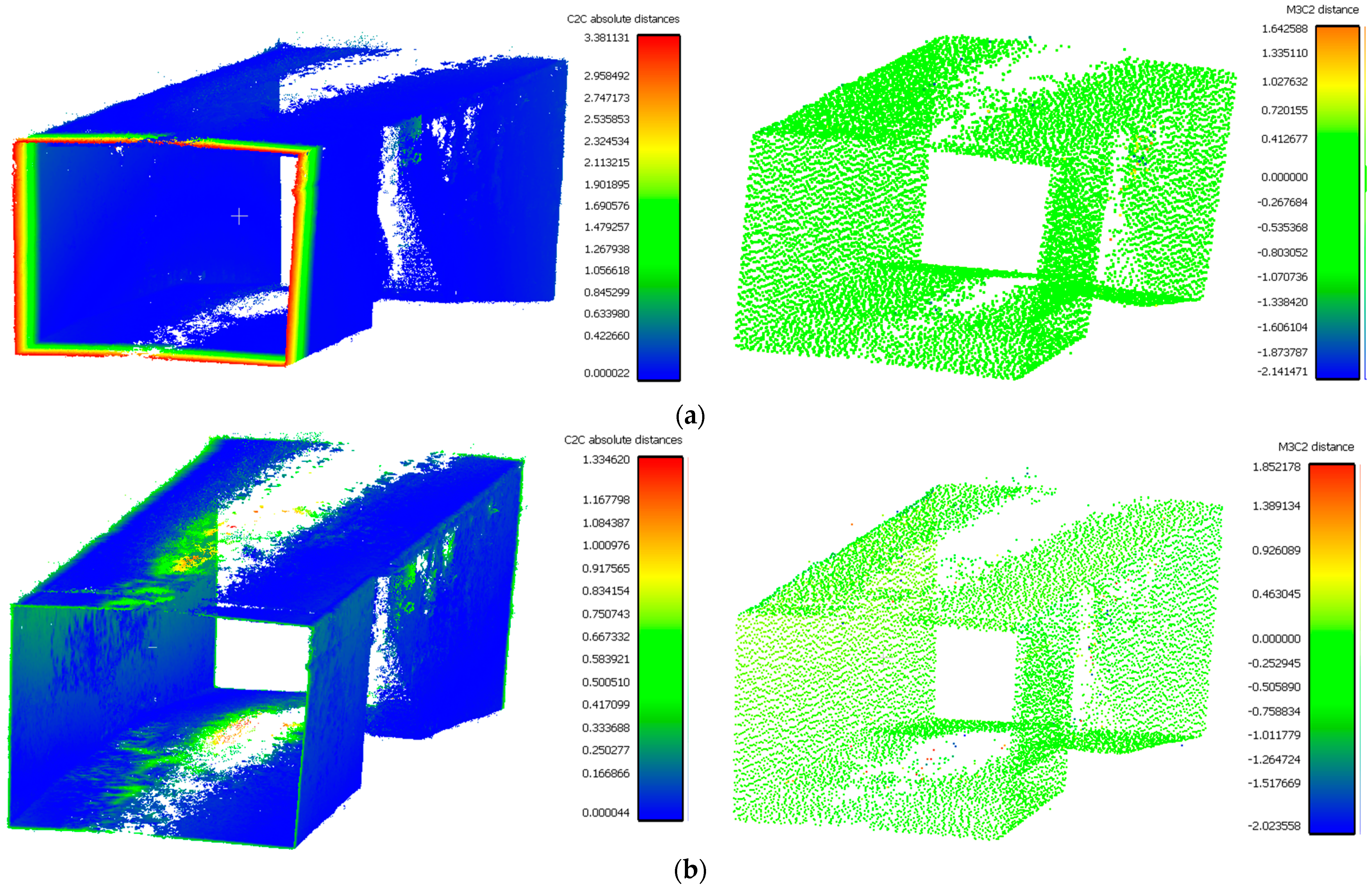
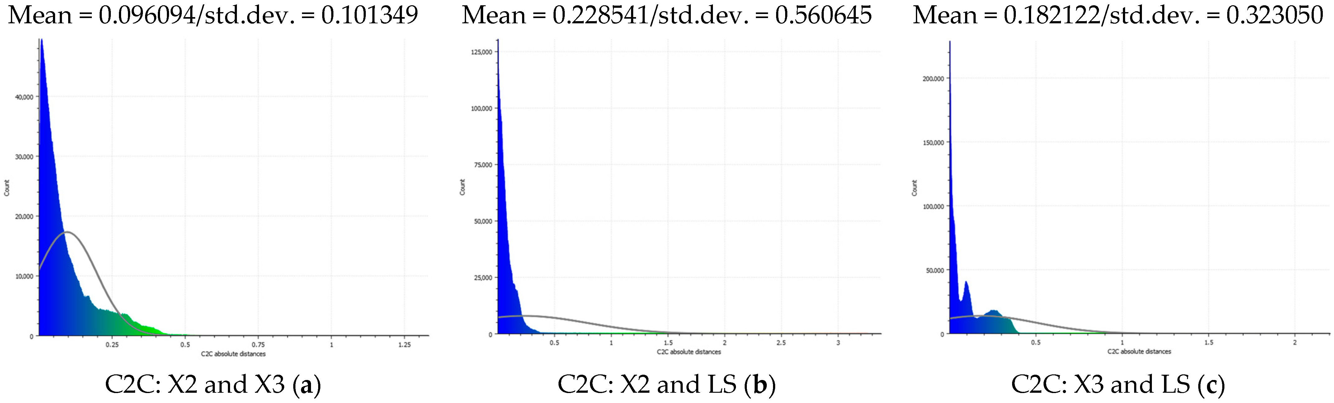
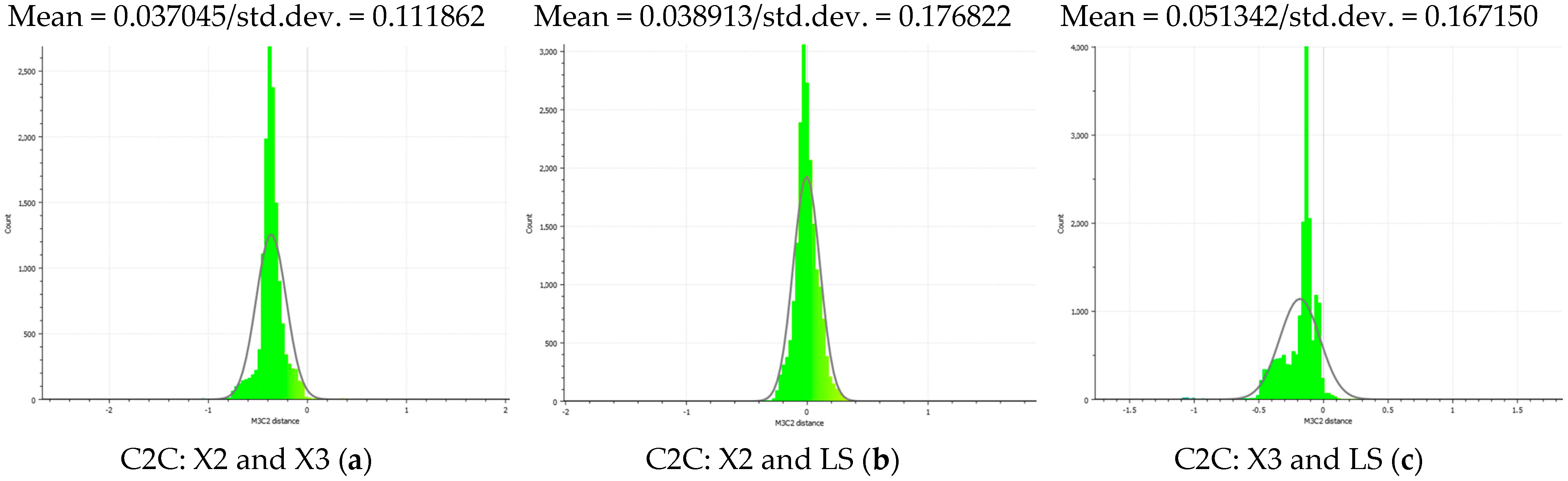
2.6.3. Distance Analysis
2.6.4. Geometric Features
3. Results
4. Discussion and Conclusions
Author Contributions
Funding
Data Availability Statement
Conflicts of Interest
References
- Wu, Y.; Zhou, Z. Intelligent City 3D Modeling Model Based on Multisource Data Point Cloud Algorithm. J. Funct. Spaces 2022, 2022, 6135829. [Google Scholar] [CrossRef]
- Karantanellis, E.; Arav, R.; Dille, A.; Lippl, S.; Marsy, G.; Torresani, L.; Oude Elberink, S. Evaluating the quality of photogrammetric point-clouds in challenging geo-environments—A case study in an alpine valley. ISPRS Int. Arch. Photogramm. Remote Sens. Spat. Inf. Sci. 2020, XLIII-B2-2020, 1099–1105. [Google Scholar]
- Pepe, M.; Alfio, V.S.; Costantino, D.; Herban, S. Rapid and Accurate Production of 3D Point Cloud via Latest-Generation Sensors in the Field of Cultural Heritage: A Comparison between SLAM and Spherical Videogrammetry. Heritage 2022, 5, 1910–1928. [Google Scholar] [CrossRef]
- Zwęgliński, T.; Smolarkiewicz, M. Three-Dimensional model and orthophotomap’s quality evaluation towards facilitating aerial reconnaissance of flood response needs. In Innovation in Crisis Management; Routledge: London, UK, 2022; pp. 215–233. [Google Scholar]
- Mendonca, P.R.S.; Cipolla, R. A simple technique for self-calibration. In Proceedings of the 1999 IEEE Computer Society Conference on Computer Vision and Pattern Recognition, Fort Collins, CO, USA, 23–25 June 1999. [Google Scholar]
- Burger, W. Zhang’s Camera Calibration Algorithm: In-Depth Tutorial and Implementation; Technical Report HGB16-05; FH OÖ: Wels, Austria, 2016. [Google Scholar]
- Pierdicca, R.; Paolanti, M.; Matrone, F.; Martini, M.; Morbidoni, C.; Malinverni, E.S.; Frontoni, E.; Lingua, A.M. Point Cloud semantic segmentation using a deep learning framework for cultural heritage. Remote Sens. 2020, 12, 1005. [Google Scholar] [CrossRef]
- Đurić, I.; Vasiljević, I.; Obradović, M.; Stojaković, V.; Kićanović, J.; Obradović, R. Comparative Analysis of Open-Source and Commercial Photogrammetry Software for Cultural Heritage. In Proceedings of the IneCAADe 2021 International Scientific Conference, Novi Sad, Serbia, 8–10 September 2021; pp. 8–10. [Google Scholar]
- Torkan, M.; Janiszewski, M.; Uotinen, L.; Baghbanan, A.; Rinne, M. Photogrammetric Method to Determine Physical Aperture and Roughness of a Rock Fracture. Sensors 2022, 22, 4165. [Google Scholar] [CrossRef] [PubMed]
- Jiang, S.; You, K.; Li, Y.; Weng, D.; Chen, W. 3D Reconstruction of Spherical Images based on Incremental Structure from Motion (Version 2). arXiv 2023, arXiv:2302.04495. [Google Scholar]
- Su, Z.; Gao, Z.; Zhou, G.; Li, S.; Song, L.; Lu, X.; Kang, N. Building plane segmentation based on point clouds. Remote Sens. 2021, 14, 95. [Google Scholar] [CrossRef]
- Madokoro, H.; Yamamoto, S.; Nishimura, Y.; Nix, S.; Woo, H.; Sato, K. Calibration and 3D Reconstruction of Images Obtained Using Spherical Panoramic Camera. In Proceedings of the 2021 21st International Conference on Control, Automation and Systems (ICCAS), Jeju, Republic of Korea, 12–15 October 2021; pp. 311–318. [Google Scholar] [CrossRef]
- Kouros, G.; Kotavelis, I.; Skartados, E.; Giakoumis, D.; Tzovaras, D.; Simi, A.; Manacorda, G. 3D Underground Mapping with a Mobile Robot and a GPR Antenna. In Proceedings of the 2018 IEEE/RSJ International Conference on Intelligent Robots and Systems (IROS), Madrid, Spain, 1–5 October 2018; pp. 3218–3224. [Google Scholar] [CrossRef]
- Chen, Y.; Medioni, G. Object Modeling by Registration of Multiple Range Images. In Proceedings of the IEEE Conference on Computer Vision and Pattern Recognition, Maui, HI, USA USA, 3–6 June 1991. [Google Scholar]
- Huang, H.-Y.; Chen, Y.-S.; Hsu, W.-H. Color image segmentation using a self-organizing map algorithm. J. Electron. Imaging 2002, 11, 136–148. [Google Scholar] [CrossRef]
- Jiang, S.; You, K.; Li, Y.; Weng, D.; Chen, W. 3D reconstruction of spherical images: A review of techniques, applications, and prospects. Geo-Spat. Inf. Sci. 2024. [Google Scholar] [CrossRef]
- Kim, J.; Kim, H.; Oh, J.; Li, X.; Jang, K.; Kim, H. Distance Measurement of Tunnel Facilities for Monocular Camera-based Localization. J. Inst. Control. Robot. Syst. 2023, 29, 7–14. [Google Scholar] [CrossRef]
- DiFrancesco, P.-M.; Bonneau, D.; Hutchinson, D.J. The Implications of M3C2 Projection Diameter on 3D Semi-Automated Rockfall Extraction from Sequential Terrestrial Laser Scanning Point Clouds. Remote Sens. 2020, 12, 1885. [Google Scholar] [CrossRef]
- Pathak, S.; Moro, A.; Fujii, H.; Yamashita, A.; Asama, H. 3D reconstruction of structures using spherical cameras with small motion. In Proceedings of the 2016 16th International Conference on Control, Automation and Systems (ICCAS), Gyeongju, Republic of Korea, 16–19 October 2016. [Google Scholar]
- Janiszewski, M.; Torkan, M.; Uotinen, L.; Rinne, M. Rapid Photogrammetry with a 360-Degree Camera for Tunnel Mapping. Remote Sens. 2022, 14, 5494. [Google Scholar] [CrossRef]
- Shi, F.; Yang, J.; Li, Q.; He, J.; Chen, B. 3D laser scanning acquisition and modeling of tunnel engineering point cloud data. J. Phys. Conf. Ser. 2023, 2425, 012064. [Google Scholar] [CrossRef]
- Morsy, S.; Shaker, A. Evaluation of LiDAR-Derived Features Relevance and Training Data Minimization for 3D Point Cloud Classification. Remote Sens. 2022, 14, 5934. [Google Scholar] [CrossRef]
- Fangi, G.; Pierdicca, R.; Sturari, M.; Malinverni, E.S. Improving Spherical Photogrammetry Using 360° Omni-Cameras: Use Cases and New Applications. Int. Arch. Photogramm. Remote Sens. Spat. Inf. Sci. 2018, 42, 331–337. [Google Scholar] [CrossRef]
- Bi, Z.; Wang, L. Advances in 3D data acquisition and processing for industrial applications. Robot. Comput.-Integr. Manuf. 2010, 26, 403–413. [Google Scholar] [CrossRef]
- Altuntaş, C. Camera Self-Calibration by Using Structure from Motion Based Dense Matching for Close-Range Images. Eurasian J. Sci. Eng. Technol. 2021, 2, 69–82. [Google Scholar]
- Xie, Y.; Tian, J.; Zhu, X.X. Linking points with labels in 3D: A review of Point Cloud Semantic Segmentation. IEEE Geosci. Remote Sens. Mag. 2020, 8, 38–59. [Google Scholar] [CrossRef]
- Herban, S.; Costantino, D.; Alfio, V.S.; Pepe, M. Use of Low-Cost Spherical Cameras for the Digitisation of Cultural Heritage Structures into 3D Point Clouds. J. Imaging 2022, 8, 13. [Google Scholar] [CrossRef] [PubMed]
- Agisoft. Agisoft Metashape User Manual: Professional Edition, version 2.1; Agisoft LLC: St. Petersburg, Russia, 2024. [Google Scholar]
- Available online: http://www.cs.unc.edu/~isenburg/pointzip/ (accessed on 18 November 2023).
- Rodríguez-Cuenca, B.; García-Cortés, S.; Ordóñez, C.; Alonso, M.C. A study of the roughness and curvature in 3D point clouds to extract vertical and horizontal surfaces. In Proceedings of the 2015 IEEE International Geoscience and Remote Sensing Symposium (IGARSS), Milan, Italy, 26–31 July 2015. [Google Scholar]
- Chen, B.; Shi, S.; Gong, W.; Zhang, Q.; Yang, J.; Du, L.; Sun, J.; Zhang, Z.; Song, S. Multispectral LiDAR Point Cloud Classification: A Two-Step Approach. Remote Sens. 2017, 9, 373. [Google Scholar] [CrossRef]
- Weinmann, M.; Jutzi, B.; Mallet, C. Feature relevance assessment for the semantic interpretation of 3D point cloud data, ISPRS Ann. Photogrammetry. Remote Sens. Spat. Inf. Sci. 2013, 2, 313–318. [Google Scholar]
- Lague, D.; Brodu, N.; Leroux, J. Accurate 3D comparison of complex topography with terrestrial laser scanner: Application to the Rangitikei canyon (N-Z). ISPRS J. Photogramm. Remote Sens. 2013, 82, 10–26. [Google Scholar] [CrossRef]
- Hackel, T.; Wegner, J.D.; Schindler, K. Contour detection in unstructured 3D point clouds. In Proceedings of the IEEE Conference on Computer Vision and Pattern Recognition, Las Vegas, Nevada, USA, 27–30 June 2016; pp. 1610–1618. [Google Scholar]
- Förstner, W.; Wrobel, B.P. Photogrammetric Computer Vision; Geometry and Computing: Geometric Feature Extraction by a Multi-Scale and Multi-Threshold Approach; Springer International Publishing: Cham, Switzerland, 2016. [Google Scholar]
- Gallup, D.; Frahm, J.-M.; Pollefeys, M. Piecewise planar and non-planar stereo for urban scene reconstruction. In Proceedings of the 2010 IEEE Computer Society Conference on Computer Vision and Pattern Recognition, San Francisco, CA, USA, 13–18 June 2010; pp. 1418–1425. [Google Scholar]


| Camera Model | Brand | Resolution (Megapixel) | Image Resolution (pix) | Weight (kg) | Raw File Accessibility | Cost (USD) | Monitoring Software |
|---|---|---|---|---|---|---|---|
| Gear360 | Samsung | 15 | 4096 × 2048 | 0.13 | ✓ | 369 | ✓ |
| Theta Z1 | Ricoh | 23 | 6720 × 3360 | 0.18 | × | 559 | × |
| Theta X | Ricoh | 60 | 11,008 × 5504 | 0.17 | ✓ | 796 | × |
| Max360 | GoPro | 16 | 5760 × 2880 | 0.16 | ✓ | 399 | ✓ |
| One X | Insta360 | 18 | 5760 × 2880 | 0.11 | × | 259 | ✓ |
| One X2 | Insta360 | 48 | 6080 × 3040 | 0.14 | ✓ | 290 | ✓ |
| One X3 | Insta360 | 18.72 | 11,968 × 5984 | 0.18 | ✓ | 399 | ✓ |
| Solutions | Network Design Solution | Data Type Solution | Calibration Solution |
|---|---|---|---|
| Solution 1 | Sideways mode | Fisheye images | Self-calibration |
| Solution 2 | Sideways mode | Fisheye images | Chessboard calibration (splitting mode) |
| Solution 3 | Sideways mode | Fisheye images | Chessboard calibration (without splitting mode) |
| Solution 4 | Sideways mode | Panorama images | --- |
| Solution 5 | Stereo mode | Fisheye images | Self-calibration |
| Solution 6 | Stereo mode | Fisheye images | Chessboard calibration (splitting mode) |
| Solution 7 | Stereo mode | Fisheye images | Chessboard calibration (without splitting mode) |
| Solution 8 | Stereo mode | Panorama images | --- |
| Laser Scanner Accuracy Settings | Values |
|---|---|
| 3D point accuracy | 1.9 mm in 10 m|2.9 mm in 20 m|5.3 mm in 40 m |
| Ground/space sampling resolution | 3 mm (highest sampling resolution) |
| Angular accuracy of LS | 18″ |
| Range accuracy | 1 mm in 10 ppm |
| Optical camera for colorized point cloud | 3 cameras, 36 MP resolution |
| Noise distance | 0.4 mm in 10 m|0.5 mm in 20 m |
| Calibration Parameters | X3 (Front Lens) | X3 (Rear Lens) | X2 (Front Lens) | X2 (Rear Lens) | D800 |
|---|---|---|---|---|---|
| F (Focal length, pix) | 1554.8544 | 1555.5011 | 848.4453 | 848.1613 | 2150.0099 |
| cx (principal point offset in X axis, pix) | −2.4490 | −1.0948 | −8.2083 | −0.4822 | −14.8078 |
| cy (principal point offset in Y axis, pix) | 20.4959 | 24.6478 | 3.7923 | −0.2146 | −3.1103 |
| K1 (radial distortion, pix) | 0.0726 | 0.0893 | 0.0515 | 0.0465 | −0.0357 |
| K2 (radial distortion, pix) | 0.0017 | −0.0424 | −0.0103 | 0.0018 | −0.0124 |
| K3 (radial distortion, pix) | −0.0246 | 0.0230 | 0.0052 | −0.0058 | 0.0316 |
| K4 (radial distortion, pix) | 0.0107 | −0.0067 | −0.0042 | −0.0003 | −0.0236 |
| B1 (non-orthogonality, pix) | −0.5308 | −0.7564 | −0.8797 | −0.8279 | 3.2830 |
| B2 (non-orthogonality, pix) | 1.2574 | 1.7960 | 0.0991 | 0.0945 | 0 |
| P1 (tangential distortion, pix) | −0.0007 | −0.0007 | 4.8196 × 10⁻⁵ | −0.0002 | −0.0001 |
| P2 (tangential distortion, pix) | −0.0007 | −0.0016 | −0.0005 | −0.0006 | −0.0010 |
| Alignment Settings | Values |
|---|---|
| Tie point threshold | 8000 |
| Key point threshold | 40,000 |
| Camera calibration methods | Two methods: Brown fisheye model (self-calibration)|Zhang’s method (chessboard calibration) |
| Accuracy mode | High|Generic preselection |
| Calibration Parameters | Reconstruction Uncertainty | Re-Projection Error | Image Count |
|---|---|---|---|
| Threshold value | 30 | ~1 | 2 |
| Sensor | Camera Orientation | RMSE Re-Projection | Calibration RMS Residual (pix) | Number of Point Clouds | Number of Tie Points |
|---|---|---|---|---|---|
| Without pre-calibration (refined during relative orientation–self-calibration) | |||||
| X2 | stereo | 0.136758 | 0.427 | 4,588,728 | 16,077/67,275 |
| X3 | stereo | 0.126319 | 0.835 | 13,875,434 | 9601/54,016 |
| X2 | sideways | 0.766283 | 1.377 | 18,676,576 | 43,782/62,556 |
| X3 | sideways | 0.343216 | 0.742 | 30,471,652 | 21,968/118,537 |
| Calibration without splitting groups (in two separate chunks) | |||||
| X2 | stereo | 0.176492 | 0.694 | 5,292,014 | 14.210/67.275 |
| X3 | stereo | 0.200214 | 3.1 | 14,747,707 | 6850/54,014 |
| X2 | sideways | 0.26795 | 1.28 | 14,242,671 | 17,238/62,431 |
| X3 | sideways | 0.4989 | 3.762 | 39,937,968 | 37,810/58,581 |
| Calibration with splitting groups (in one chunk) | |||||
| X2 | stereo | 0.27507 | 1.364 | 6,388,632 | 26,857/54,185 |
| X3 | stereo | 0.37041 | 1.226 | 10,652,336 | 5514/57,984 |
| X2 | sideways | 0.24312 | 1.083 | 14,118,170 | 35,312/57,520 |
| X3 | sideways | 0.32965 | 2.357 | 37,484,289 | 32,946/56,378 |
| Calibration | RMSE Re-Projection | Calibration RMS Residual (pix) | Number of Point Clouds | Number of Tie Points |
|---|---|---|---|---|
| Not calibrated | 0.165979 | 0.158 | 42,193,069 | 14,306/29,616 |
| Calibrated | 0.32821 | 1.56 | 11,542,445 | 15,136/29,614 |
| Sensor | Camera Orientation | RMSE Re-Projection | Number of Point Clouds | Number of Tie Points |
|---|---|---|---|---|
| X2 | stereo | 0.702747 | 9,489,270 | 19,518/57,564 |
| X3 | stereo | 0.268801 | 17,671,659 | 21,288/42,700 |
| X2 | sideways | 0.282473 | 11,542,445 | 28,341/37,765 |
| X3 | sideways | 0.414831 | 40,166,750 | 6456/26,155 |
| Sensor | Camera Orientation | GCP Accuracy (m) | Check Point Accuracy (m) |
|---|---|---|---|
| without calibration (being refined during relative orientation) | |||
| X2 | stereo | 0.003592 | 0.047857 |
| X3 | stereo | 0.027332 | 0.100306 |
| X2 | sideways | 0.102562 | 0.7241114 |
| X3 | sideways | 0.001714 | 0.010127 |
| calibration without splitting groups (in two separate chunks) | |||
| X2 | stereo | 0.068918 | 0.368897 |
| X3 | stereo | 0.056098 | 0.504710 |
| X2 | sideways | 0.066433 | 0.453532 |
| X3 | sideways | 0.045880 | 0.079698 |
| calibration with splitting groups (in one chunk) | |||
| X2 | stereo | 0.01 | 0.06 |
| X3 | stereo | 0.02 | 0.13 |
| X2 | sideways | 0.01 | 0.07 |
| X3 | sideways | 0.04 | 0.13 |
| Compared Clouds | C2C Distance Measurement | M3C2 Distance Measurement | ||
|---|---|---|---|---|
| Std. Deviation | Mean Distance | Std. Deviation | Mean Distance | |
| X2 and X3 | 0.101 | 0.096 | 0.176 | 0.038 |
| X2 and LS | 0.560 | 0.228 | 0.111 | 0.037 |
| X3 and LS | 0.323 | 0.181 | 0.167 | 0.051 |
| X2 and DSLR | 0.342 | 0.152 | 0.077 | 0.015 |
| X3 and DSLR | 1.171 | 0.91 | 0.083 | 0.007 |
| Geometric Features | Insta360 One X3 | Insta360 One X2 | Laser Scanner | DSLR Camera |
|---|---|---|---|---|
| Roughness |  |  |  |  |
| Density |  |  |  |  |
| Verticality |  |  |  |  |
| Planarity |  |  |  |  |
| Linearity | 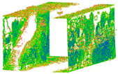 | 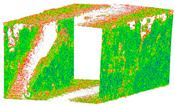 |  | 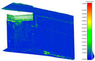 |
| Curvature |  | 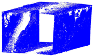 |  |  |
Disclaimer/Publisher’s Note: The statements, opinions and data contained in all publications are solely those of the individual author(s) and contributor(s) and not of MDPI and/or the editor(s). MDPI and/or the editor(s) disclaim responsibility for any injury to people or property resulting from any ideas, methods, instructions or products referred to in the content. |
© 2024 by the authors. Licensee MDPI, Basel, Switzerland. This article is an open access article distributed under the terms and conditions of the Creative Commons Attribution (CC BY) license (https://creativecommons.org/licenses/by/4.0/).
Share and Cite
Rezaei, S.; Maier, A.; Arefi, H. Quality Analysis of 3D Point Cloud Using Low-Cost Spherical Camera for Underpass Mapping. Sensors 2024, 24, 3534. https://doi.org/10.3390/s24113534
Rezaei S, Maier A, Arefi H. Quality Analysis of 3D Point Cloud Using Low-Cost Spherical Camera for Underpass Mapping. Sensors. 2024; 24(11):3534. https://doi.org/10.3390/s24113534
Chicago/Turabian StyleRezaei, Sina, Angelina Maier, and Hossein Arefi. 2024. "Quality Analysis of 3D Point Cloud Using Low-Cost Spherical Camera for Underpass Mapping" Sensors 24, no. 11: 3534. https://doi.org/10.3390/s24113534