Abstract
The use of low-cost environmental sensors has gained significant attention due to their affordability and potential to intensify environmental monitoring networks. These sensors enable real-time monitoring of various environmental parameters, which can help identify pollution hotspots and inform targeted mitigation strategies. Low-cost sensors also facilitate citizen science projects, providing more localized and granular data, and making environmental monitoring more accessible to communities. However, the accuracy and reliability of data generated by these sensors can be a concern, particularly without proper calibration. Calibration is challenging for low-cost sensors due to the variability in sensing materials, transducer designs, and environmental conditions. Therefore, standardized calibration protocols are necessary to ensure the accuracy and reliability of low-cost sensor data. This review article addresses four critical questions related to the calibration and accuracy of low-cost sensors. Firstly, it discusses why low-cost sensors are increasingly being used as an alternative to high-cost sensors. In addition, it discusses self-calibration techniques and how they outperform traditional techniques. Secondly, the review highlights the importance of selectivity and sensitivity of low-cost sensors in generating accurate data. Thirdly, it examines the impact of calibration functions on improved accuracies. Lastly, the review discusses various approaches that can be adopted to improve the accuracy of low-cost sensors, such as incorporating advanced data analysis techniques and enhancing the sensing material and transducer design. The use of reference-grade sensors for calibration and validation can also help improve the accuracy and reliability of low-cost sensor data. In conclusion, low-cost environmental sensors have the potential to revolutionize environmental monitoring, particularly in areas where traditional monitoring methods are not feasible. However, the accuracy and reliability of data generated by these sensors are critical for their successful implementation. Therefore, standardized calibration protocols and innovative approaches to enhance the sensing material and transducer design are necessary to ensure the accuracy and reliability of low-cost sensor data.
1. Introduction
Climate change is a significant challenge for environmental sustainability [1,2], and to address this issue effectively, it is crucial to advance scientific knowledge by collecting and comprehending information on various aspects related to climate change [3]. This requires a comprehensive understanding of the global environmental system and data collection is the most crucial part of this process.
The environment is facing significant challenges worldwide, particularly in terms of pollution which substantially degrades it. These challenges are largely due to a combination of factors, including population growth, the ageing of infrastructure, the impacts of climate change, and ongoing global development [4,5]. Environmental pollution including water, air and soil pollution has become prevalent globally. More research needs to be conducted to effectively monitor and understand the sources, concentrations, and effects of environmental pollutants to aid policymakers and citizens in developing strategies for preventing pollution and protecting the environment, particularly in vulnerable regions.
Thus, there is an urgent need to develop a more effective and rapid method of monitoring environmental pollution given that the traditional methods of collecting data and samples which often involve laboratory analysis are expensive, time-consuming, and labour-intensive. Also, traditional data collection methods are not real-time and lack the fast data collection and dissemination which are needed for an effective and timely response to protect the environment [6,7]. The traditional method of monitoring the environment, e.g., water and air quality parameters, involves manual collection of samples from different areas and carrying out several laboratory analyses to process, analyse and characterise samples. These traditional methods for environmental monitoring are now seen as inadequate for effectively monitoring the environment, partly because they are also prone to human error [6,8]. This has led to several researchers emphasising the need for developing low-cost, robust, and standard methods and sensors for identifying and quantifying pollutants in the environment.
Environmental attributes such as the quality of water, air, and soil are usually observed through traditional sensors located at established monitoring stations. These conventional in-situ methods, employing stationary sensors, come with limitations in data resolution and necessitate intensive training and maintenance. Meanwhile, when using satellite data, challenges arise due to disparities in spatial and temporal scales compared to environmental occurrences [9]. Furthermore, the need for increased data collection density has surged over the last two decades, driven by population growth and escalating levels of air and water pollution.
Recent advancements in digital electronics, wireless communication technologies, and sensor manufacturing [10] have generated a growing demand within the field of environmental science for low-cost sensor networks (LCSNs). These networks are increasingly valuable for addressing both fundamental research inquiries and practical management challenges [11,12]. This shift in approach is driven by the accessibility of low-cost sensors (LCSs) equipped with user-friendly technologies and calibration methods that yield data with enhanced spatial resolution [13,14,15]. Several factors, including the decreased costs of microcontrollers for sensors, environmental sensor components, and straightforward communication modules, have played pivotal roles in bringing about this shift. Additionally, the expanded spatial coverage afforded by LCSs enables the generation of fresh insights into environmental dynamics [16].
The term ‘low-cost’ sensor does not define a specific price range, as the cost can vary depending on the specific parameters being measured. It can be defined as a sensor that is relatively inexpensive to produce, purchase, and maintain compared to other sensors with similar functionalities [14].
Low-cost sensors are the latest and most innovative technology used in monitoring water and air quality in real time. The use of low-cost sensors for environmental sensing and monitoring is increasing due to the availability and affordability of low-cost sensors, internet facilities, and cloud computing services [8,17]. Low-cost sensors also require fewer human interventions to operate and thus are less biased compared to traditional techniques and can be deployed in remote and inaccessible locations.
Wireless network sensors, for example, have become popularly employed by researchers for environmental monitoring of factors such as water quality parameters e.g., temperature, pH, dissolved oxygen, turbidity, water flow rate, and conductivity [18,19]. They have also been used to measure air quality parameters such as particulate matter, carbon monoxide, and nitrogen dioxide [20,21]. For example, in the past 10 years, studies such as [6,22] have attached water and air quality sensors, respectively, to Arduino controllers; an open-source, user-friendly, and simple platform to measure and monitor water quality parameters including dissolved oxygen, pH, temperature, nitrates, and turbidity in their studies.
The real-time water quality data from the above studies were acquired, processed, and automatically transmitted through Internet of Things (IoT) systems. A network of low-cost sensors that can collect real-time data will aid in the detection and understanding of the sources and pathways of pollution in the environment large and remote. This will be significant in effectively modelling and monitoring the vulnerability of human health and the ecosystem to environmental pollution.
However, any sensor that is more affordable than the instrumentation needed to meet regulatory requirements for the parameter under study is categorized as low-cost [22]. In this context, the cost of sensors typically increases when additional components such as microprocessors, data loggers, memory cards, batteries, and display units are incorporated.
The increased adoption of low-cost sensors (LCSs) in recent studies can be attributed to the user-friendly nature of these sensors, which allows for a cost-effective expansion of spatial coverage that has been traditionally limited. While the existing literature acknowledges the value of LCSs as a valuable addition to the commonly used measurement tools, it consistently highlights the potential for sensor misuse leading to more frequent inaccuracies. It is important to note that data collected from these sensors are indicative of specific locations and their ambient conditions, suggesting underlying factors affecting sensor measurements. In essence, the selectivity of a sensor refers to its ability to differentiate between the intended target and any interfering elements [23]. For example, a gas sensor designed to detect one type of particle often exhibits sensitivity to other particles, which can interfere with the accurate measurement of the target pollutant or particle. This phenomenon is known as sensor cross-sensitivity and can be assessed by exposing the sensor to other pollutants [24].
A standard reference sensor tends to show a higher sensitivity to particles, therefore is more precise, and more selective to measure a specific variable of interest. Therefore, according to WMO reports, low-cost sensors should be used under established quality assurance and quality control protocols [25,26,27]. Further, a more precise calibration approach will be attained with selectivity and sensitivity of a low-cost sensor at any location. Therefore, to use an LCS instrument, a published standard set of criteria must be followed which should be provided by regulatory agencies. Selectivity and sensitivity are two essential factors to take into account while considering an LCS for any given investigation.
Low-cost sensors with higher spatial resolution can provide us with better regional accuracy and offer us even more liberty to choose the variables that are appropriate for the region. The existing literature demonstrates, however, that low-cost sensors suffer from significant uncertainties because of large data outliers, weak correlations, and low data precision [28,29]. The selectivity of the sensors may improve the evaluation, but more thorough calibration procedures that address the difficulties that have been raised can produce improved results.
Sensor calibration is the process of comparing the output of the instrument or sensor under test against the output of an instrument of known accuracy when the same input is applied to both instruments [30] by developing a mathematical function that describes the relationship between the uncalibrated variables and the reference [28]. However, the relationship between uncalibrated and reference is not a direct proportion; there exists the influence of multiple other parameters. Therefore, the calibration function can be improved by utilising cross-sensitive parameters that influence the parameter of interest. Automatic and semi-automatic calibration methods are two calibration methods that are largely used for LCSs [13,28,31,32]. This review article aims to answer several questions related to the increasing popularity of low-cost sensors as an alternative to high-cost sensors. The article explores why selectivity and sensitivity of sensors are crucial factors in low-cost sensors, and how calibration functions can improve accuracy. Additionally, the article discusses ways to enhance the accuracy of sensors, providing insights into the development of low-cost sensing technologies.
2. Literature Survey Approach
The literature survey is conducted in a structured approach which covers identification, screening, eligibility assessment, and final inclusion. The PRISMA Statement, which outlines the Preferred Reporting Items for Systematic reviews and Meta-Analyses, was the principal criterion used in this study. PRISMA can be defined as guidelines that provide a structured framework for authors to follow when writing and reporting systematic reviews and meta-analyses [33]. Its use by Cochrane Collaboration defines the systematic review as “an examination of a clearly formulated questions that uses systematics and explicit methods to identify, select, and critically appraise relevant research and to collect and analyse data from the studies that are included in the review. Statistical methods may or may not be used to analyse and summarise the results of the included studies” [34,35]. The primary search criteria applied for identification of the articles in each database are as follows: “(“water quality” or “air quality” AND ‘low-cost sensors’ AND “calibration”)” and with time-period 2013 to 2022. The number of articles identified from the databases SCOPUS, Science Direct, and Web of Science are 127, 12, and 1, respectively. The returned articles were uploaded to the Rayyan online platform [36] for screening and preselection of publications for further review of articles. We excluded papers that were not in English, unpublished, or duplicates, resulting in 70 papers being selected for further review. In the subsequent phase, eight of the authors independently evaluated the title, abstract, and conclusions of these 70 papers based on specific inclusion and exclusion criteria detailed in Table 1 to determine their relevance. This process identified 46 relevant papers and a thorough full-text review of the 46 shortlisted papers was conducted. To write this study, we looked at more than just the aforementioned papers and book chapters to determine the types of sensors for each relevant parameter since there are numerous sensors made explicitly for monitoring specific parameters. The PRISMA diagram as applicable to this systematic review study is shown in Figure 1.

Table 1.
Inclusion and exclusion criteria used for the systematic review.
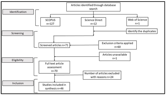
Figure 1.
Flowchart for the selection and screening of the articles.
3. LCSs for Monitoring Air and Water Quality
This article looks at the calibration and validation methods of low-cost sensors with exclusive focus on water and air quality sensors. Table 2 provides a number of selected key studies related to the use of LCSs on air and water quality. The literature shows that in the past decade, the use of LCSs for air-quality assessment has improved rapidly.
Table 2.
Summary of articles considered for the review.
3.1. LCSs for Air Quality
The selection of LCSs for air quality depends upon the parameter of interest and its characteristic. For instance, sensors for particulate matter (PM) and gaseous pollutants (GL) are different. Furthermore, the cross-sensitivity of the parameter also plays a major role in selecting the sensor. International and national level health organisations have created several protocols for standardised pollutants in the air. For example, the World Health Organisation (WHO) has updated a global air quality guideline for both particulate matter and gaseous pollutants in the air; in the European Union (EU), as part of the ‘European Green Deal’ proposed directives that align with WHO standards, the directive 2011/850/EU [65] is the most recent legislation passed to reduce pollution concentration thresholds. Sensors for measuring air quality can be broadly divided into two groups: (1) sensors for estimating particulate matter concentrations (PMx), and (2) sensors for estimating gaseous contaminants in ambient air. In the sections that follow, we go over them.
3.1.1. LCSs for Particulate Matter
PM is a mixture of airborne solid particles and liquid droplets that can be inhaled with air. Particle mass concentration (Pmass) and particle number concentration (Pnum) are the two basic metrics used to measure atmospheric particulate matter (PM). Pnum is the number of particles in a given volume (particles/cm3), and Pmass is the mass of the particles in a given volume (typically g/cm3) [66]. PM in general is characterised by its shape, size, and composition (Table 3). The diameter of the particle sub-categorises PM; for example, PM2.5 and PM10 are for particulate matter of diameter 2.5 and 10 micrometres, respectively. The particle concentration (either mass or number) is measured throughout a range of different particle sizes and is referred to as the particle size distribution (Psd).
Table 3.
Particulate matter characteristics.
Currently, a typical commercially available LCS for PM sensing uses the light-scattering principle, with the sensor consisting of three major components: a light emitting diode, photo-transistor, and a lens to focus the diode light [67,68].
The common reference/validation techniques for LCSs monitoring PM are ‘Tapered Element Oscillation Microbalance’ (TEOM) and ‘Beta Attenuation Monitor’ (BAM), both of which measure properties directly associated with Pmass [69].
3.1.2. LCSs for Gaseous Pollutants
Gaseous pollutants include the following pollutants in their gaseous state emitted by, for example, an engine: carbon monoxide (CO), total hydrocarbons (HC), oxides of nitrogen (NOx), and other greenhouse gases (GHG); NOx being nitric oxide (NO) and nitrogen dioxide (NO2), expressed as NO2 equivalent, and GHG includes carbon dioxide (CO2), methane (CH4), and nitrous oxide (N2O) [70,71,72]. The gas sensors detect the presence of these pollutants (gas concentrations) in the environment using different sensing materials. The main objective of gas sensor development is to establish an array of multifunctional gas sensor technologies that can monitor air pollution at a low cost and be used to create an electronic nose [73]. Different types of gas sensors include electrochemical sensors, metal-oxide semiconductors, catalytic combustion type, acoustic-wave based, and optical gas sensors [73,74] and the selection depends on the gas types, which can be flammable, combustible, and toxic. These sensors are chosen for their affordability, portability, elegant design, limited sensitivity, and selectivity, and the requirement for extra equipment [75] during use. Among them, metal-oxide semiconductor sensors are particularly popular due to their several unique features, such as high sensitivity, rapid response and recovery times, simple manufacturing process, robust stability, easy operation, and low expense [74,75]. Table 4 lists several sensors used for air-quality measurements. PurpleAir is the most used LCS for air-quality parameters due to its easily accessible and cost-effective approach.
Table 4.
Various low-cost sensor models used for air-quality monitoring from the literature.
3.2. LCSs for Water Quality
The quality of water determined by its chemical, physical, and biological properties plays an important role in human health. Monitoring water characteristics including conductivity, pH, salinity, temperature, dissolved oxygen, residual chlorine, and turbidity is essential to maintaining its quality; therefore, water quality monitors are widely used.
Just like in air-quality monitoring, international and national-level health organisations have created several protocols for a standardised range for monitoring water quality. For instance, the Guidelines for Drinking Water Quality (GDWQ) are produced by the World Health Organization (WHO) through regular revisions, of which the most recent is the GDWQ 4th edition. Europe established its own water quality norms by adapting from WHO guidelines known as EU Water Framework Directives (WFD), the most recent being Directive 2006/118/EC [65]. The challenge of maintaining water quality standards is great, and continuous monitoring using a conventional approach is cost-effective and often unable to produce real-time data. Low-cost water quality sensors can overcome this constraint whilst enhancing the spatial density of data. Primary cost components of water quality sensors are designing, installing sensors with power supply utility, communication equipment, access, lighting, security, and environmental conditions of the location.
Two primary approaches for water quality measurement are direct measurement of constituents, and surrogate measurement which are chemical concentrations that indicate the presence of undesired contaminants in the water [78,79]. The following are the most common water quality sensors used to measure key parameters:
3.2.1. Chlorine Residual Sensor
The most popular method of disinfection to lessen water contamination is chlorination. The theory of chlorination is straightforward: When chlorine comes into direct contact with microorganisms in water, it destroys their cellular structure, causing disinfection. Monitoring residual chlorine, which refers to the effective chlorine remaining in water after chlorination, is generally essential to mitigate the risk of chlorine residuals [80]. Although adding a lot of chlorine to the treated water will increase disinfection efficiency, doing so can also cause unpleasant odours, formation of a lot of carcinogenic disinfection by-products, faster distribution system corrosion, and certain health hazards [80,81]. Electrochemical sensors (amperometry and ion-selective electrodes), spectrophotometric sensors (colourimetry and fluorescence), and biosensors are the three main chlorine residual monitoring devices Amperometry sensors, which track changes in current, are the most economical and widely used sensors [82,83]. Moreover, these sensors trigger less with the presence of dissolved oxygen, temperature, pH, and other oxidants than do biosensors and fluorescence sensors.
3.2.2. Total Organic Carbon (TOC) Sensor
TOC measures organic compounds in pure water and aqueous systems and is primarily used in treating wastewater and testing drinking water contamination. The fundamental methods for measuring TOC are based on organic matter oxidation to detect CO2 through conductometry and IR spectroscopy [84,85]; however, the process is time-consuming and expensive. Through low-cost sensors it is possible to monitor TOC regularly, rapidly, and with affordability. Campanella et al. 2002 [85] developed a sensor that measures the amount of CO2 created by the UV-assisted photodegradation of organic matter which is improved by nanosized TiO2 (anatase). TiO2 anatase is a colourless, metastable mineral form of titanium dioxide, which is a suitable photocatalyst in the photodegradation of toxic organic molecules due to its high activity, nontoxicity, and chemical inertness [86], and it is widely regarded as the most suitable photocatalyst for TOC contamination studies [86,87,88].
3.2.3. Turbidity Sensor
Turbidity is the most highlighted parameter, which is also known as haziness of a fluid due to suspended solids [89]. The WHO [90] standard for turbidity in ideal drinking water is below 1 NTU (Nephelometric Turbidity Units), as higher levels of turbidity in water produce favourable conditions for contagious pathogens [91]. As in other water quality measures, the fundamental approach to turbidity monitoring is through laboratory analysis due to its reliability and accuracy. However, these products are economically unviable at large scale, therefore for such products spatio-temporal scales reduce drastically, which is not viable for continuous monitoring. Further, these systems require significant preparation and regular management.
Low-cost sensors filling these gaps and mostly used for turbidity are developed with other sensing parameters such as dissolved oxygen, Ph, phosphorous, etc. Low-cost turbidity sensors typically use transmitted light detection (optical sensor) to monitor the haziness of water, though the accuracy and reliability of these sensors can be lower [92].
3.2.4. Conductivity Sensor
Significant increases in water conductivity indicate that the water is contaminated, unsafe for drinking, and may harm aquatic creatures. Conductivity comes under physical water quality parameters like turbidity, hardness, and temperature. With advancing technologies, sensors that measures the conductivity of water can be made rapidly using materials that are readily available; however, the price of a conductivity sensor is still too costly for good coverage of spatial resolution [93].
3.2.5. pH and ORP Sensors
The pH of water indicates alkalinity characteristics, whereas ORP (Oxygen-reduction Potential) gives an insight into the level of oxidation/reduction reactions occurring in the water. The pH for drinking water should be between 6.5 and 8.5, whereas ORP is not a mandatory parameter according to WHO and EU standards. However, the ORP value is a valuable parameter to estimate the physicochemical properties of water [94]. The ORP is primarily useful to check the oxygen reductions happening in water due to contamination. Electrodes are usually used to analyse these two parameters. Both parameters come under the inorganic category [95] and are inversely proportional to each other, which means as pH decreases, ORP increases, and vice-versa [94].
Most water quality parameters are measurable with higher accuracies using conventional laboratory assessments. However, this time-consuming task is not feasible for monitoring of large spatial networks and real-time values. With the advancements in sensor technologies, an overarching approach has been developed to study a selected range of parameters depending upon the geographical location, risks, and usual contamination history. Several attempts have been made to identify a range of water quality parameters with sensor technology; nevertheless, Internet of Things (IoT) has been the most recent advancement in continuous monitoring of water quality. Sensing of parameters like pH, turbidity, temperature, conductivity, and dissolved oxygens are regularly monitored using IoT. [96] developed IoT to track water quality using Thing Speak (IoT technology) which sends data from numerous sensors to Arduino via the cloud.
Lakshmikantha et al. 2021 [97] introduced LED additions to an IoT-based water monitoring system which is connected to a Raspberry Pi using Java. Several sensors were used to determine the range of water quality, and accordingly these LEDs lit up. Salunke & Kate 2017 [98] developed a sensor network with the Intel Galileo Gen 2 board to test water monitoring and demonstrated improved results. On an application to assess agriculture water quality, Paepae (et al., 2021) [99] used a virtual sensing system to demonstrate physical sensor methods with clear results. These water quality sensors typically are exposed to environmental conditions such as rainfall, dust, and wind. To overcome this challenge, [63] developed a 3D printing system, with a method of fabrication which is durable in the long term. Brewin et al. 2019 [62], developed a pocket-size hand-held device with marine-resistant materials using a 3D printer to measure water clarity and colour in lakes, estuaries, and nearshore regions. Despite the fact that these innovations are brand new for IoT sensor applications for water-quality measurement, there is a lot of room for improvement in terms of artificial algorithms for accurate calibration.
4. Self-Calibration Techniques
Self-calibration techniques refer to methods and processes that enable a system, device, or instrument to automatically calibrate itself without the need for external reference standards or manual intervention [100]. They have been gaining attention in various fields, including engineering, metrology, and sensor technologies [100]. These techniques are particularly valuable in situations where traditional calibration methods may be impractical, time-consuming, or cost-prohibitive [101]. Self-calibration techniques are employed in various fields such as in-situ calibration, sensor fusion, machine learning calibration, and environmental monitoring [15,102,103,104].
Studies by [15,24,102,105,106,107] highlight the numerous benefits of self-calibration techniques. These advantages include real-time adjustment capabilities, allowing for continuous monitoring and adjustment of measurement equipment to maintain accuracy over time. Unlike traditional calibration methods, self-calibration reduces the need for human intervention, minimizing downtime and interruptions to equipment operation. Additionally, self-calibration enhances accuracy by continuously monitoring and correcting measurement deviations, reducing the risk of drift or changes between calibration sessions. Automation in calibration processes also decreases the likelihood of human error, ensuring more consistent and reliable calibration results. Moreover, self-calibration systems adapt to environmental changes and operating conditions, maintaining accuracy despite variations in external factors. While initial implementation may require investment, the potential for reduced manual labour and increased efficiency offers long-term cost savings.
Self-calibration methods vary depending on the type of sensor and the specific factors being addressed. For instance, the approach for self-calibration differs between chlorine sensors and sensors for gases like CO or HC [108]. These methods typically comprise several steps to ensure precise and dependable measurements. For example, zero calibration is the initial step, involving placing the sensor in a solution with zero chlorine concentration, such as deionized water, to establish a baseline reading. This calibrates the sensor to a reference point in the absence of chlorine. Subsequently, span calibration requires immersing the sensor in a known concentration of chlorine solution to calibrate its response at a specific chlorine concentration. Adjustments are then made by comparing sensor readings with expected values at zero and span calibration points, aligning the sensor output accordingly. Regular maintenance checks and calibrations are crucial for monitoring sensor accuracy over time, considering factors like sensor drift, environmental conditions, and aging. Some advanced chlorine sensors may provide automated calibration features or routines, necessitating adherence to the manufacturer’s instructions for effective utilization. Finally, verifying sensor performance involves testing it with known chlorine concentrations to ensure ongoing accuracy and reliability. These steps collectively ensure the precision and functionality of chlorine sensors for environmental monitoring applications.
Although there are multiple advantages in self-calibration methods, they do have some drawbacks in terms of accuracy, limited calibration range, and maintenance requirements [108]. It is important to recognize that the sensor’s properties undergo gradual changes over time, resulting in decreased accuracy. Therefore, regular calibration is essential to maintain precision. Additionally, determining the optimal calibration frequency depends on the specific application and is typically established through practical experience.
It is also crucial to acknowledge that self-calibration procedures may not be suitable for all applications or industries [109]. Traditional calibration methods, involving manual calibration by qualified specialists on a regular basis, remain prevalent and trusted in many industries [110].
5. Calibration Techniques and Developments in Their Accuracy
The design of an experiment and its sensor calibration methods may be more effectively directed if it is understood how LCSs differ from standard instruments. A widely reported issue with LCSs is that they suffer from large uncertainties relating to low data precision and accuracy [28,30,31,51]. This uncertainty in performance can be related to various limitations such as low-signal-to-noise ratios for different sensors, environmental factors, and low selectivity. Due to the different types of air quality sensors used, it is often difficult to compare data from different studies. For example, the same air quality parameter (PM2.5) was measured in similar sites in Nairobi, Kenya by Kiai et al. 2021, and Pope et al. 2018 [51,111]. However, there was a difference in the scaling factor used for calibration of the low-cost sensors and this can mainly be related to the differences in the type of low-cost sensors used [51].
In order to address these difficulties, LCSs may need extensive calibration processes. Sensor calibration is defined as ‘a process to determine the mathematical function (calibration function) that defines the relation between independent and dependent variable’. There are various methods used to obtain calibration data, for example, field calibration and laboratory calibration. For low-cost sensors, the calibration processes generally employed are automatic and semi-automatic techniques. The literature shows several methods that have been used to validate the calibrations obtained from LCSs, such as Tapered Element Oscillating Microbalance (TEOM), nephelometer, GRIMM EDM 180 monitor, and predominantly a gravimetric Federally Equivalent Method (FEM) instrument known as Attenuation Monitor (BAM).
Calibration models are applied during pre-deployment of sensors to deal with errors that occur in mapping raw sensor measurements; the fundamental methods here are offset and gain calibration [112]. ‘Gain’ describes the sensor’s response to rising pollutant concentrations, and ‘offset’ describes the sensor’s response to total absence of the target pollutant. In combination, they create the calibration curve.
For instance, Shi et al. 2021 [93] performed a simple one-point calibration before the sensor deployment (Equation (1)), the calibration offset here is the difference between air and depth sensors.
where d is water depth (m), pabs is the absolute pressure (mbar), pair is the ambient air pressure (mbar), ecal is the calibration offset (mbar) and ρwater is the density of water at a specific temperature (kg/m3), and g is the gravitational acceleration constant (9.81 m/s2).
There are other errors reported from the environment such as temperature, wind speed, relative humidity, and turbulence. Fang & Bate 2017 [28] studied cross-sensitive parameters between multiple parameters (Equation (2)) by adding the interaction terms into the calibration function. However, they concluded that using only a single parameter to calibrate low-cost sensors in urban environments is likely to be insufficient.
where Y is the dependent variable, X1 and X2 are independent variables which can be noise, and β is the calibration coefficient.
Data evaluation in LCSs typically includes outlier detection, inter-sensor comparisons, and comparison with traditional monitors [113], all of which contribute to data loss for a network, reducing the spatial resolution. Table 5 provides a summary of low-cost sensors from the literature review and the standard validation and accuracy methods employed in their studies. For instance, Fienberg developed a network of 20 sensor pods to study air quality at the Shelby Farm monitoring site, where three sensors never operated, six failed during operation, and with R2 threshold of 0.5, only six sensor pods met the data quality objective. Such sensor failure and data loss has been detected from other sensor networks as well [48,113,114,115]. Outlier detection is defined as the detection of values that are statistically significantly distinct from the other normal values at a given time and location [113]. Detection of outliers is a crucial element in finding erroneous values and removing them; they occur due to faults in sensors, weather patterns, and dirt attachment to sensors. For assessment of air-quality sensors, many calibration models, primarily Linear Regression (LR), Multivariate Linear Regression (MLR), or a variety of Machine Learning (ML) algorithms, including artificial neural networks, random forests, and support vector regression, among others, were used [29,116].
Water quality monitoring sensors are mostly deployed in water for a long period of time, therefore require protection from fouling/biofouling which leads to uncertainty in values [8]. Various studies [8,117,118] indicated that biofouling may be the cause for degraded water quality monitoring data, and their proposed solution is to design sensor nodes that are suitable for wiper cleaning. Another calibration uncertainty in water quality sensors is due to sensor drift, a temporal shift in the sensor’s response under constant physical and chemical conditions brought on by sensor damage from water pressure and water fluxes [119]. The literature showed that the major drawback concerning non-contact LCSs is practically observed [63] when the turbidity sensor stopped function after one month due to attachment of dirt such as mud/silt/microorganisms which need to be cleaned off regularly. Therefore, a sensor with a self-cleaning mechanism can improve the calibration results. Further, higher linearities for the signals received from sensors compared to actual measurements indicate a reduction in accuracy. Wong et al. 2021 [63] developed a 3D-printed water quality sensor which showed turbidity within the range of 10 to 1000 FNU and gives more accurate results, where optimum measurement ranges for the ultrasonic and temperature sensors are 2–400 cm and 10–50 °C, respectively. Calibration techniques mentioned in Table 5 provide insights into the calibration of both air quality and water quality sensors, including techniques such as MBE, RMSE, determination of correction factors of optical sensors using cyclone samplers, nephelometer, linear regression equation, MLR, LR, ANN, Mini-Vol configuration, correlations, ordinary least square regression, FRM, FEM, multiple linear regression, etc.
Table 5.
Summary of low-cost sensors from the literature review and the standard validation and accuracy methods employed in their studies.
Table 5.
Summary of low-cost sensors from the literature review and the standard validation and accuracy methods employed in their studies.
| Author Ref. | Location | Calibration Methods Used | |
|---|---|---|---|
| Standard Measurement Validation | Calibration Techniques | ||
| Air Quality | |||
| [44] | Patras city in Greece | Compared with GRIMM EDM 180 monitor. | MBE, eMBE, rMAE, RMSE, R2. |
| [51] | Kenya | A standard Andersen dichotomous impactor (Sierra Instruments Inc., Monterey, CA, USA) was used to calibrate the low-cost sensors for four days by collocation. | Correction factor of the optical sensors (PMS7003) was determined from the cyclone samplers (BGI 400S). |
| [52] | Australia | The PurpleAir (PA-II) low-cost sensors were collocated with three reference sensors: Tapered Element Oscillating Microbalance (TEOM), nephelometer, DustTrak monitors. | TEOM sensors were related to the nephelometer using an equation. The low-cost sensors were calibrated (hourly and daily) using a relationship (equation) with the nephlometer and TEOM. |
| [53] | USA | TEOM federal equivalent method (FEM) monitor was used for reference sensor and collocation. | Linear Regression equation for the reference monitor (TEOM) and the low-cost sensors. |
| [54] | USA | A Met One Beta Attenuation Monitor (BAM); a gravimetric FEM instrument was used as the reference monitor and collocation. | Least squares linear regression, MBE, MAE. |
| [55] | USA, Rwanda, Malawi and DR Congo | BAMs were used as the reference monitor and collocation. | Linear regression, MAE. |
| [29] | Serbia | Automatic Monitoring Station (AMS) Stari Grad was used as the reference monitor and collocation. | NRMSE, LR, MLR, MBE and ANN Square Difference (uRMSD). |
| [56] | Palestine, Nablus | AirUs were calibrated for local PM using a filter-based, low-volume air sampler Mini-Vol configured for PM2.5 collection. | Mini-Vol configured for PM2.5 collection. |
| [50] | Australia | Correlation between the KOALA and TEOM over a 12-month period. | (R2 = 0.89), >0.90 for the daily averages between the TEOM and KOALA for PM2.5. |
| [49] | N/A | Fan-based. | Correlations (R). |
| [120] | USA | Calibration performed with reference to a reference ozone analyser (Thermo 49i), is manufactured by Thermo Fisher Scientific, located in Waltham, MA, USA | Ordinary least squares (OLS) regression. |
| [121] | China | Calibration and validation were performed with reference to US federal reference methods (FRMs; TEOM-FDMS, BAM, SHARP). | Linear regression, RH adjusted linear regression. |
| [122] | USA | Calibration and validation was performed with reference to federal equivalent method (BAM). | Multiple linear regression with the BAM PM2.5, RH, and T as predictors. |
| [58] | USA | Validation with reference to federal reference method (FRM). | Validation with reference to federal reference method (FRM) and federal equivalent method (FEM) monitors. |
| [123] | USA | Proxy model developed from a reference instrument. | Proxy corrected sensor data and K-means clustering. |
| Water quality | |||
| [61] | Taihu Lake and Yuqiao Reservoir | Based on synchronous measurements with a field spectrometer, the results were validated. | RMSE, MRE, R2. |
| [62] | UK and destinations in the South Atlantic | An iButton temperature logger was attached to the mini-secchi disk and it was calibrated against a NIST-traceable (and NPL-traceable) Hart Scientific. | Comparison between the housed iButton and the NIST-traceable probe with the difference in average, median, absolute average, median absolute in N number of samples. |
Linear regression (LR), Normalized Root Mean Squared Error (NRMSE), Multivariate linear regression (MLR), Mean Bias Error (MBE), Mean Absolute Error (MAE), and Artificial Neural Network (ANN), Coefficient of correlation (R), coefficient of determination (R2).
Most of the current studies utilizing low-cost sensors for air pollution measurement use simple linear regression to calibrate low-cost sensors in relation to the reference device to improve accuracy. However, linear regression cannot model this relationship since several non-linear and environmental variables can affect the accuracy of low-cost sensors [29]. Thus, to truly account for these variables, machine learning techniques may prove very useful [46,68,107].
There are several metrics that were employed to estimate the accuracy of sensor monitored values (Table 6). These metrics are designed to capture the main aspects of the time-series behaviours. The accuracy between these sensors and standard measures changes due to the seasons, location, and meteorological/water quality conditions of air/water. The accuracy of Plantower PMS7003 sensors was evaluated by Kiai et al. 2021 [51] and they showed that the sensor’s level of accuracy is high; earlier studies on Plantower sensors demonstrated better accuracies as well. These studies aid scientists and other interested parties in choosing a low-cost sensor for their research.
Table 6.
Summary of accuracy assessment formulae from literature.
Rapid changes in meteorological conditions/water quality affects a sensor’s detected values and when the accuracy is assessed, the sensor shows large fluctuations [63,124].
From the literature, it can be seen that the calibration for any such LCS should be carried out using five primary indicators. They are (i) environment and its condition, (ii) pollutant/contaminant parameter(s) to be monitored, (iii) sensor specifications with its lower and higher accuracy range, (iv) validation instrument that was/were to be used, and (v) the type of regression model/models one uses to study the parameters [16].
6. Conclusions and Future Research Directions
This review article thoroughly explores the complex domain of low-cost sensors (LCSs), particularly those designed for monitoring air and water quality. The study also provides a brief insight into their advancements and barriers. Emphasizing the crucial contribution of LCSs to environmental research and public health, the discussion highlights their growing availability and cost-effectiveness as key facilitators.
Improved technologies and efforts in understanding environmental pollution are making low-cost sensors more available for research and understanding of the environment. The current study reveals that recent research has focused heavily on PM sensors in relation to air quality sensing. This may be due to the affordability of low-cost PM sensors and the growing public awareness of the health crisis caused by air pollution. However, these inexpensive sensors have faced significant difficulties due to the capital costs associated with installation, communication networks, maintenance, and the instruments for data interpretation [10].
The study also showed that, in contrast to air pollution, there is little research being done on the potential of water quality sensors. This may be as a result of a lack of regulations pertaining to water quality sensor technologies, as well as poorly defined categories of contaminants and exposure levels. The usage of LCSs in water quality applications, however, may rise as a result of growing concern over poor water quality and the cost benefits associated. To give good results, and to avoid malfunctioning, it is recommended to use sensors with a self-cleaning mechanism. For water quality measurement, the need for low-cost sensor devices with antifouling characteristics should be investigated and developed for commercial use [8], and additionally, standard algorithms for sensor drift should be developed [119]. However, these facilities demand a good power source and self-cleaning mechanism, which again is not adequately attainable with inexpensive sensors. For measurement of air pollution, several studies revealed that meteorological parameters such as relative humidity (RH), temperature (T), pressure (P), and wind impact the performance of low-cost sensors and therefore there is a need to use standard reference-grade monitoring stations for evaluation and validation. It is further advised to not rely on low-cost air-quality sensors at higher RH value locations [125].
In addition, the study also summarized self-calibration techniques and their contribution to enhancing accuracy, efficiency, and reliability. Calibrating low-cost environmental sensors presents both challenges and opportunities in the realm of air and water quality monitoring. While these sensors offer cost-effective solutions and increased spatial data density, they often suffer from uncertainties related to accuracy and precision. Challenges such as sensor drift, environmental factors, and limited calibration ranges underscore the need for robust calibration techniques. Various calibration methods, including automatic and semi-automatic techniques, have been employed to address these challenges, with a focus on offset and gain calibration models. Despite these challenges, advancements in self-calibration techniques and machine learning algorithms offer promising opportunities to improve sensor accuracy and reliability over time. Studies have highlighted the benefits of self-calibration, such as real-time adjustment capabilities and reduced reliance on manual intervention, leading to increased efficiency and cost savings in the long run. Additionally, machine learning algorithms have potential to act as a powerful tool for modelling complex relationships between sensor readings and environmental variables, enhancing the accuracy of low-cost sensor measurements.
The literature study further reveals that most of the correlations used were of the R square form and RMSE for measurement error analysis. Further, the accuracy of the sensors depends upon the environmental conditions, geological location, standard reference used, and the regression models [16]. Further, the literature review showed that Purple Air is the most used for air quality whereas many experiments on water quality have relied on IoT to monitor multiple parameters.
There is still a lack of regulatory bodies to maintain gathered data and oversee processing and usage of data for these sensors. Regular processing and maintenance of LCSs for commercial entities and scientific bodies is very challenging due to limited budgets. Citizen-owned networks with regulatory bodies may help to overcome part of this challenge.
To build confidence in low-cost sensors for real-world monitoring, regular calibration and validation with a co-located standard instrument is critical [125]. Improved statistical methods, IoT-based platforms, and space-based sensors can all improve methodological approaches for environmental pollution. Additionally, an inclusive approach using installed LCSs, standard measuring units, remote sensing, smart networks with effective communication, and data preservation can constitute best practice, while cutting-edge computational techniques like machine learning can make it easier to make a reliable forecast estimate for the future. For IoT sensors, an optimum maintenance time is required to ensure performance and cost-effectiveness of the system. Although there are still many issues related to LCSs that need to solved, their potential has been expanding due to the growing need for a clean environment and the climate change crisis in addition to the need to involve citizens in monitoring the local environment. The participation of citizens and their recognition of the obligation to maintain pollution metrics, such as indoor, outdoor air quality and water quality, has markedly expanded LCSs at the citizen level and is contributing to further advancements in sensor technologies.
However, it is essential to recognize that calibration procedures may not be suitable for all applications, and traditional calibration methods remain prevalent in many industries. Furthermore, ongoing research is needed to address the limitations of low-cost sensors, such as sensor drift and environmental factors, and to develop standardized calibration protocols for widespread adoption.
Author Contributions
Conceptualization: N.V.S.R.N., S.G., I.A. (Iulia Anton) and K.R.; Methodology: N.V.S.R.N., I.A. (Ismaila Abimbola), T.A., I.A. (Iulia Anton), K.R., Q.I., A.B., A.T. and S.G.; Software: K.R.; Validation: N.V.S.R.N., I.A. (Ismaila Abimbola) and S.G.; Formal analysis: N.V.S.R.N.; Investigation: N.V.S.R.N. and Q.I.; Resources: N.V.S.R.N.; Data curation: I.A. (Iulia Anton), K.R. and N.V.S.R.N.; Writing—original draft preparation: N.V.S.R.N., I.A. (Ismaila Abimbola), K.R., I.A. (Iulia Anton), A.B., T.A. and A.T.; Writing—review and editing: N.V.S.R.N.; Visualization: N.V.S.R.N.; Supervision: S.G., I.A. (Iulia Anton) and N.V.S.R.N.; Project administration: S.G. and N.V.S.R.N.; Funding acquisition: S.G. All authors have read and agreed to the published version of the manuscript.
Funding
The research project for this article has received funding from the European Union’s Horizon 2020 research and innovation programme under grant agreement No 101003534. This output reflects the views of the authors, and the European Commission is not responsible for any use that may be made of the information contained therein.
Institutional Review Board Statement
Not applicable.
Informed Consent Statement
Not applicable.
Data Availability Statement
Data are contained within the article.
Conflicts of Interest
The authors declare no conflict of interest.
References
- Klingelhöfer, D.; Müller, R.; Braun, M.; Brüggmann, D.; Groneberg, D.A. Climate change: Does international research fulfill global demands and necessities? Environ. Sci. Eur. 2020, 32, 137. [Google Scholar] [CrossRef] [PubMed]
- Lehtonen, A.; Salonen, A.O.; Cantell, H. Climate change education: A new approach for a world of wicked problems. In Sustainability, Human Well-Being, and the Future of Education; Springer: Cham, Switzerland, 2018. [Google Scholar] [CrossRef]
- Faghmous, J.H.; Kumar, V. A Big Data Guide to Understanding Climate Change: The Case for Theory-Guided Data Science. Big Data 2014, 2, 155–163. [Google Scholar] [CrossRef] [PubMed]
- Tran, H.M.; Tsai, F.J.; Lee, Y.L.; Chang, J.H.; Chang, L.T.; Chang, T.Y.; Chung, K.F.; Kuo, H.P.; Lee, K.Y.; Chuang, K.J.; et al. The impact of air pollution on respiratory diseases in an era of climate change: A review of the current evidence. Sci. Total Environ. 2023, 898, 166340. [Google Scholar] [CrossRef] [PubMed]
- Ameen, R.F.M.; Mourshed, M. Urban environmental challenges in developing countries—A stakeholder perspective. Habitat Int. 2017, 64, 1–10. [Google Scholar] [CrossRef]
- Lambrou, T.P.; Anastasiou, C.C.; Panayiotou, C.G.; Polycarpou, M.M. A low-cost sensor network for real-time monitoring and contamination detection in drinking water distribution systems. IEEE Sens. J. 2014, 14, 2765–2772. [Google Scholar] [CrossRef]
- Chen, S. Study on Real-Time Monitoring Method of Marine Ecosystem Micro-Plastic Pollution. J. Coast. Res. 2020, 95, 1032. [Google Scholar] [CrossRef]
- Adu-Manu, K.S.; Tapparello, C.; Heinzelman, W.; Katsriku, F.A.; Abdulai, J.D. Water quality monitoring using wireless sensor networks: Current trends and future research directions. ACM Trans. Sens. Netw. 2017, 13, 1–41. [Google Scholar] [CrossRef]
- Chan, K.; Schillereff, D.N.; Baas, A.C.W.; Chadwick, M.A.; Main, B.; Mulligan, M.; O’Shea, F.T.; Pearce, R.; Smith, T.E.L.; van Soesbergen, A.; et al. Low-cost electronic sensors for environmental research: Pitfalls and opportunities. Prog. Phys. Geogr. 2021, 45, 305–338. [Google Scholar] [CrossRef]
- Kumar, P.; Morawska, L.; Martani, C.; Biskos, G.; Neophytou, M.; Di Sabatino, S.; Bell, M.; Norford, L.; Britter, R. The rise of low-cost sensing for managing air pollution in cities. Environ. Int. 2015, 75, 199–205. [Google Scholar] [CrossRef]
- Benedetti, M.; Ioriatti, L.; Martinelli, M.; Viani, F. Wireless Sensor Network: A Pervasive Technology for Earth Observation. IEEE J. Sel. Top. Appl. Earth Obs. Remote Sens. 2010, 3, 488–496. [Google Scholar] [CrossRef]
- Mao, F.; Khamis, K.; Krause, S.; Clark, J.; Hannah, D.M. Low-Cost Environmental Sensor Networks: Recent Advances and Future Directions. Front. Earth Sci. 2019, 7, 221. [Google Scholar] [CrossRef]
- Fisher, R.; Ledwaba, L.; Hancke, G.; Kruger, C. Open hardware: A role to play in wireless sensor networks? Sensors 2015, 15, 6818–6844. [Google Scholar] [CrossRef]
- Karagulian, F.; Barbiere, M.; Kotsev, A.; Spinelle, L.; Gerboles, M.; Lagler, F.; Redon, N.; Crunaire, S.; Borowiak, A. Review of the performance of low-cost sensors for air quality monitoring. Atmosphere 2019, 10, 506. [Google Scholar] [CrossRef]
- Ojha, T.; Misra, S.; Raghuwanshi, N.S. Wireless sensor networks for agriculture: The state-of-the-art in practice and future challenges. Comput. Electron. Agric. 2015, 118, 66–84. [Google Scholar] [CrossRef]
- Kang, Y.; Aye, L.; Ngo, T.D.; Zhou, J. Performance evaluation of low-cost air quality sensors: A review. Sci. Total Environ. 2022, 818, 151769. [Google Scholar] [CrossRef]
- Kale, A.; Chaczko, Z. iMuDS: An internet of multimodal data acquisition and analysis systems for monitoring urban waterways. In Proceedings of the 25th International Conference on Systems Engineering, ICSEng, Las Vegas, NV, USA, 22–23 August 2017; Volume 2017. [Google Scholar]
- Lopez-Ramirez, G.A.; Aragon-Zavala, A. Wireless Sensor Networks for Water Quality Monitoring: A Comprehensive Review. IEEE Access 2023, 11, 95120–95142. [Google Scholar] [CrossRef]
- Ahmedi, F.; Ahmedi, L. Dataset on water quality monitoring from a wireless sensor network in a river in Kosovo. Data Brief 2022, 44, 108486. [Google Scholar] [CrossRef] [PubMed]
- Khedo, K.; Perseedoss, R.; Mungur, A. A Wireless Sensor Network Air Pollution Monitoring System. Int. J. Wirel. Mob. Netw. 2010, 2, 31–45. [Google Scholar] [CrossRef]
- Christakis, I.; Tsakiridis, O.; Kandris, D.; Stavrakas, I. Air Pollution Monitoring via Wireless Sensor Networks: The Investigation and Correction of the Aging Behavior of Electrochemical Gaseous Pollutant Sensors. Electronics 2023, 12, 1842. [Google Scholar] [CrossRef]
- Rai, A.C.; Kumar, P.; Pilla, F.; Skouloudis, A.N.; Di Sabatino, S.; Ratti, C.; Yasar, A.; Rickerby, D. End-user perspective of low-cost sensors for outdoor air pollution monitoring. Sci. Total Environ. 2017, 607–608, 691–705. [Google Scholar] [CrossRef]
- Wusiman, M.; Taghipour, F. Methods and mechanisms of gas sensor selectivity. Crit. Rev. Solid State Mater. Sci. 2022, 47, 416–435. [Google Scholar] [CrossRef]
- Narayana, M.V.; Jalihal, D.; Shiva Nagendra, S.M. Establishing A Sustainable Low-Cost Air Quality Monitoring Setup: A Survey of the State-of-the-Art. Sensors 2022, 22, 394. [Google Scholar] [CrossRef]
- Lewis, A.; Peltier, W.R.; von Schneidemesser, E. Low-Cost Sensors for the Measurement of Atmospheric Composition: Overview of Topic and Future Applications; World Meteorological Organization (WMO): Geneva, Switzerland, 2018. [Google Scholar]
- Peltier, R.; Casterll, N.; Clements, A.; Dye, T.; Huglin, C.; Kroll, J.; Lung, S.C.; Ning, Z.; Parsons, M.; Penza, M.; et al. An Update on Low-Cost Sensors for the Measurement of Atmospheric Composition; World Meterological Organization (WMO): Geneva, Switzerland, 2021. [Google Scholar]
- García, E.; Ponluisa, N.; Quiles, E.; Zotovic-Stanisic, R.; Gutiérrez, S.C. Solar Panels String Predictive and Parametric Fault Diagnosis Using Low-Cost Sensors. Sensors 2022, 22, 332. [Google Scholar] [CrossRef]
- Fang, X.; Bate, I. Using multi-parameters for calibration of low-cost sensors in urban environment. In Proceedings of the International Conference on Embedded Wireless Systems and Networks, Uppsala, Sweden, 20–22 February 2017. [Google Scholar]
- Topalović, D.B.; Davidović, M.D.; Jovanović, M.; Bartonova, A.; Ristovski, Z.; Jovašević-Stojanović, M. In search of an optimal in-field calibration method of low-cost gas sensors for ambient air pollutants: Comparison of linear, multilinear and artificial neural network approaches. Atmos. Environ. 2019, 213, 640–658. [Google Scholar] [CrossRef]
- Morris, A.S.; Langari, R. Calibration of measuring sensors and instruments. In Measurement and Instrumentation; Academic Press: Cambridge, MA, USA, 2021. [Google Scholar] [CrossRef]
- Balzano, L.; Nowak, R. Blind Calibration of Sensor Networks. In Proceedings of the 2007 6th International Symposium on Information Processing in Sensor Networks, Cambridge, MA, USA, 25–27 April 2007. [Google Scholar] [CrossRef]
- Bychkovskiy, V.; Megerian, S.; Estrin, D.; Potkonjak, M. A collaborative approach to in-place sensor calibration. In Proceedings of the Information Processing in Sensor Networks: Second International Workshop, IPSN 2003, Palo Alto, CA, USA, 22–23 April 2003; Volume 2634. [Google Scholar] [CrossRef]
- Prill, R.; Karlsson, J.; Ayeni, O.R.; Becker, R. Author guidelines for conducting systematic reviews and meta-analyses. Knee Surg. Sports Traumatol. Arthrosc. 2021, 29, 2739–2744. [Google Scholar] [CrossRef]
- Higgins, J.P.T.; Thomas, J.; Chandler, J.; Cumpston, M.; Li, T.; Page, M.J.; Welch, V.A. Cochrane Handbook for Systematic Reviews of Interventions; John Wiley & Sons, Ltd: Hoboken, NJ, USA, 2019. [Google Scholar] [CrossRef]
- Sierra-Correa, P.C.; Cantera Kintz, J.R. Ecosystem-based adaptation for improving coastal planning for sea-level rise: A systematic review for mangrove coasts. Mar. Policy 2015, 51, 385–393. [Google Scholar] [CrossRef]
- Ouzzani, M.; Hammady, H.; Fedorowicz, Z.; Elmagarmid, A. Rayyan-a web and mobile app for systematic reviews. Syst. Rev. 2016, 5, 210. [Google Scholar] [CrossRef]
- Dhammapala, R.; Basnayake, A.; Premasiri, S.; Chathuranga, L.; Mera, K. PM2.5 in Sri Lanka: Trend Analysis, Low-cost Sensor Correlations and Spatial Distribution. Aerosol Air Qual. Res. 2022, 22, 210266. [Google Scholar] [CrossRef]
- Peters, D.R.; Popoola, O.A.M.; Jones, R.L.; Martin, N.A.; Mills, J.; Fonseca, E.R.; Stidworthy, A.; Forsyth, E.; Carruthers, D.; Dupuy-Todd, M.; et al. Evaluating uncertainty in sensor networks for urban air pollution insights. Atmos. Meas. Tech. 2022, 15, 321–334. [Google Scholar] [CrossRef]
- Cavellin, L.D.; Weichenthal, S.; Tack, R.; Ragettli, M.S.; Smargiassi, A.; Hatzopoulou, M. Investigating the Use of Portable Air Pollution Sensors to Capture the Spatial Variability of Traffic-Related Air Pollution. Environ. Sci. Technol. 2016, 50, 313–320. [Google Scholar] [CrossRef]
- Han, I.; Symanski, E.; Stock, T.H. Feasibility of using low-cost portable particle monitors for measurement of fine and coarse particulate matter in urban ambient air. J. Air Waste Manag. Assoc. 2017, 67, 330–340. [Google Scholar] [CrossRef]
- Papapostolou, V.; Zhang, H.; Feenstra, B.J.; Polidori, A. Development of an environmental chamber for evaluating the performance of low-cost air quality sensors under controlled conditions. Atmos. Environ. 2017, 171, 82–90. [Google Scholar] [CrossRef]
- Reece, S.; Williams, R.; Colón, M.; Southgate, D.; Huertas, E.; O’shea, M.; Iglesias, A.; Sheridan, P. Spatial-temporal analysis of PM2.5 and NO2 concentrations collected using low-cost sensors in Peñuelas, Puerto Rico. Sensors 2018, 18, 4314. [Google Scholar] [CrossRef]
- Kim, S.; Park, S.; Lee, J. Evaluation of performance of inexpensive laser based PM2.5 sensor monitors for typical indoor and outdoor hotspots of South Korea. Appl. Sci. 2019, 9, 1947. [Google Scholar] [CrossRef]
- Kosmopoulos, G.; Salamalikis, V.; Pandis, S.N.; Yannopoulos, P.; Bloutsos, A.A.; Kazantzidis, A. Low-cost sensors for measuring airborne particulate matter: Field evaluation and calibration at a South-Eastern European site. Sci. Total Environ. 2020, 748, 141396. [Google Scholar] [CrossRef]
- Kuula, J.; Mäkelä, T.; Aurela, M.; Teinilä, K.; Varjonen, S.; González, Ó.; Timonen, H. Laboratory evaluation of particle-size selectivity of optical low-cost particulate matter sensors. Atmos. Meas. Tech. 2020, 13, 2413–2423. [Google Scholar] [CrossRef]
- Connolly, R.E.; Yu, Q.; Wang, Z.; Chen, Y.H.; Liu, J.Z.; Collier-Oxandale, A.; Papapostolou, V.; Polidori, A.; Zhu, Y. Long-term evaluation of a low-cost air sensor network for monitoring indoor and outdoor air quality at the community scale. Sci. Total Environ. 2022, 807, 150797. [Google Scholar] [CrossRef]
- Jacob, M.T.; Michaux, K.N.; Bertrand, B.; Yvette Flore, T.S.; Nasser, N.; Vitrice Ruben, F.S.; Ruth Line, T.M. Saïdou Low-cost air quality monitoring system design and comparative analysis with a conventional method. Int. J. Energy Environ. Eng. 2021, 12, 873–884. [Google Scholar] [CrossRef]
- Miskell, G.; Alberti, K.; Feenstra, B.; Henshaw, G.S.; Papapostolou, V.; Patel, H.; Polidori, A.; Salmond, J.A.; Weissert, L.; Williams, D.E. Reliable data from low cost ozone sensors in a hierarchical network. Atmos. Environ. 2019, 214, 116870. [Google Scholar] [CrossRef]
- Mui, W.; Der Boghossian, B.; Collier-Oxandale, A.; Boddeker, S.; Low, J.; Papapostolou, V.; Polidori, A. Development of a Performance Evaluation Protocol for Air Sensors Deployed on a Google Street View Car. Environ. Sci. Technol. 2021, 55, 1477–1486. [Google Scholar] [CrossRef]
- Kuhn, T.; Jayaratne, R.; Thai, P.K.; Christensen, B.; Liu, X.; Dunbabin, M.; Lamont, R.; Zing, I.; Wainwright, D.; Witte, C.; et al. Air quality during and after the Commonwealth Games 2018 in Australia: Multiple benefits of monitoring. J. Aerosol Sci. 2021, 152, 105707. [Google Scholar] [CrossRef]
- Kiai, C.; Kanali, C.; Sang, J.; Gatari, M. Spatial Extent and Distribution of Ambient Airborne Particulate Matter (PM2.5) in Selected Land Use Sites in Nairobi, Kenya. J. Environ. Public Health 2021, 2021, 4258816. [Google Scholar] [CrossRef]
- Robinson, D.L. Accurate, low cost PM2.5 measurements demonstrate the large spatial variation in wood smoke pollution in Regional Australia and improve modeling and estimates of health costs. Atmosphere 2020, 11, 856. [Google Scholar] [CrossRef]
- Feinberg, S.N.; Williams, R.; Hagler, G.; Low, J.; Smith, L.; Brown, R.; Garver, D.; Davis, M.; Morton, M.; Schaefer, J.; et al. Examining spatiotemporal variability of urban particulate matter and application of high-time resolution data from a network of low-cost air pollution sensors. Atmos. Environ. 2019, 213, 579–584. [Google Scholar] [CrossRef]
- Feenstra, B.; Papapostolou, V.; Hasheminassab, S.; Zhang, H.; Boghossian, B.D.; Cocker, D.; Polidori, A. Performance evaluation of twelve low-cost PM2.5 sensors at an ambient air monitoring site. Atmos. Environ. 2019, 216, 116946. [Google Scholar] [CrossRef]
- Malings, C.; Tanzer, R.; Hauryliuk, A.; Saha, P.K.; Robinson, A.L.; Presto, A.A.; Subramanian, R. Fine particle mass monitoring with low-cost sensors: Corrections and long-term performance evaluation. Aerosol Sci. Technol. 2020, 54, 160–174. [Google Scholar] [CrossRef]
- Khader, A.; Martin, R.S. Use of low-cost ambient particulate sensors in Nablus, Palestine with application to the assessment of regional dust storms. Atmosphere 2019, 10, 539. [Google Scholar] [CrossRef]
- Feinberg, S.; Williams, R.; Hagler, G.S.W.; Rickard, J.; Brown, R.; Garver, D.; Harshfield, G.; Stauffer, P.; Mattson, E.; Judge, R.; et al. Long-term evaluation of air sensor technology under ambient conditions in Denver, Colorado. Atmos. Meas. Tech. 2018, 11, 4605–4615. [Google Scholar] [CrossRef]
- Collier-Oxandale, A.; Feenstra, B.; Papapostolou, V.; Zhang, H.; Kuang, M.; Der Boghossian, B.; Polidori, A. Field and laboratory performance evaluations of 28 gas-phase air quality sensors by the AQ-SPEC program. Atmos. Environ. 2020, 220, 117092. [Google Scholar] [CrossRef]
- Eidam, E.F.; Langhorst, T.; Goldstein, E.B.; McLean, M. OpenOBS: Open-source, low-cost optical backscatter sensors for water quality and sediment-transport research. Limnol. Oceanogr. Methods 2022, 20, 46–59. [Google Scholar] [CrossRef]
- Matos, T.; Faria, C.L.; Martins, M.S.; Henriques, R.; Gomes, P.A.; Goncalves, L.M. Development of a cost-effective optical sensor for continuous monitoring of turbidity and suspended particulate matter in marine environment. Sensors 2019, 19, 4439. [Google Scholar] [CrossRef]
- Gao, M.; Li, J.; Zhang, F.; Wang, S.; Xie, Y.; Yin, Z.; Zhang, B. Measurement of water leaving reflectance using a digital camera based on multiple reflectance reference cards. Sensors 2020, 20, 6580. [Google Scholar] [CrossRef]
- Brewin, R.J.W.; Brewin, T.G.; Phillips, J.; Rose, S.; Abdulaziz, A.; Wimmer, W.; Sathyendranath, S.; Platt, T. A printable device for measuring clarity and colour in lake and nearshore waters. Sensors 2019, 19, 936. [Google Scholar] [CrossRef]
- Wong, Y.J.; Nakayama, R.; Shimizu, Y.; Kamiya, A.; Shen, S.; Muhammad Rashid, I.Z.; Nik Sulaiman, N.M. Toward industrial revolution 4.0: Development, validation, and application of 3D-printed IoT-based water quality monitoring system. J. Clean. Prod. 2021, 324, 129230. [Google Scholar] [CrossRef]
- Zeng, R.; Mannaerts, C.M.; Shang, Z. A low-cost digital colorimetry setup to investigate the relationship between water color and its chemical composition. Sensors 2021, 21, 6699. [Google Scholar] [CrossRef]
- World Health Organization. WHO Global Air Quality Guidelines: Particulate Matter (PM2.5 and PM10), Ozone, Nitrogen Dioxide, Sulfur Dioxide and Carbon Monoxide; World Health Organization: Geneva, Switzerland, 2021. [Google Scholar]
- Lowther, S.D.; Jones, K.C.; Wang, X.; Whyatt, J.D.; Wild, O.; Booker, D. Particulate Matter Measurement Indoors: A Review of Metrics, Sensors, Needs, and Applications. Environ. Sci. Technol. 2019, 53, 11644–11656. [Google Scholar] [CrossRef]
- Giordano, M.R.; Malings, C.; Pandis, S.N.; Presto, A.A.; McNeill, V.F.; Westervelt, D.M.; Beekmann, M.; Subramanian, R. From low-cost sensors to high-quality data: A summary of challenges and best practices for effectively calibrating low-cost particulate matter mass sensors. J. Aerosol Sci. 2021, 158, 105833. [Google Scholar] [CrossRef]
- Wang, Y.; Li, J.; Jing, H.; Zhang, Q.; Jiang, J.; Biswas, P. Laboratory Evaluation and Calibration of Three Low-Cost Particle Sensors for Particulate Matter Measurement. Aerosol Sci. Technol. 2015, 49, 1063–1077. [Google Scholar] [CrossRef]
- Bulot, F.M.J.; Johnston, S.J.; Basford, P.J.; Easton, N.H.C.; Apetroaie-Cristea, M.; Foster, G.L.; Morris, A.K.R.; Cox, S.J.; Loxham, M. Long-term field comparison of multiple low-cost particulate matter sensors in an outdoor urban environment. Sci. Rep. 2019, 9, 7497. [Google Scholar] [CrossRef]
- Li, C.; Feng, S.; Qiu, X.; Guo, G.; Zhang, E.; He, Q.; He, X.; Ma, W.; Fittschen, C. Palm-sized laser spectrometer with high robustness and sensitivity for trace gas detection using a novel double-layer toroidal cell. Anal. Chem. 2021, 93, 4552–4558. [Google Scholar] [CrossRef]
- Hayashi, D.; Sakaguchi, Y.; Minami, M. Control of gas concentration distribution in a semiconductor process chamber using CT-TDLAS measurement. AIP Adv. 2021, 11, 025034. [Google Scholar] [CrossRef]
- Zhu, Y.; Shen, X.; Zhou, M.; Su, X.; Li, J.; Yang, G.; Shao, H.; Zhou, Y. Ultra-broadband 1.0 μm band emission spectroscopy in Pr3+/Nd3+/Yb3+ tri-doped tellurite glass. Spectrochim. Acta Part A Mol. Biomol. Spectrosc. 2019, 222, 117178. [Google Scholar] [CrossRef] [PubMed]
- Soo, K. Gas Sensors for Monitoring Air Pollution. In Monitoring, Control and Effects of Air Pollution; IntechOpen: London, UK, 2011. [Google Scholar] [CrossRef]
- Gomes, J.B.A.; Rodrigues, J.J.P.C.; Rabêlo, R.A.L.; Kumar, N.; Kozlov, S. IoT-enabled gas sensors: Technologies, applications, and opportunities. J. Sens. Actuator Netw. 2019, 8, 57. [Google Scholar] [CrossRef]
- Majhi, S.M.; Mirzaei, A.; Kim, H.W.; Kim, S.S.; Kim, T.W. Recent advances in energy-saving chemiresistive gas sensors: A review. Nano Energy 2021, 79, 105369. [Google Scholar] [CrossRef]
- Muis, S.; Apecechea, M.I.; Dullaart, J.; de Lima Rego, J.; Madsen, K.S.; Su, J.; Yan, K.; Verlaan, M. A High-Resolution Global Dataset of Extreme Sea Levels, Tides, and Storm Surges, Including Future Projections. Front. Mar. Sci. 2020, 7, 263. [Google Scholar] [CrossRef]
- Weissert, L.; Alberti, K.; Miles, E.; Miskell, G.; Feenstra, B.; Henshaw, G.S.; Papapostolou, V.; Patel, H.; Polidori, A.; Salmond, J.A.; et al. Low-cost sensor networks and land-use regression: Interpolating nitrogen dioxide concentration at high temporal and spatial resolution in Southern California. Atmos. Environ. 2020, 223, 117287. [Google Scholar] [CrossRef]
- Horowitz, A.J. A review of selected inorganic surface water quality-monitoring practices: Are we really measuring what we think, and if so, are we doing it right? Environ. Sci. Technol. 2013, 47, 2471–2486. [Google Scholar] [CrossRef] [PubMed]
- KIL, J. Introduction of residual chlorine sensor using constant voltage method and its measurement principles. Eur. J. Mater. Sci. Eng. 2021, 6, 113–118. [Google Scholar] [CrossRef]
- Lin, T.-F.; Watson, S.; Dietrich, A.M.; Suffet, I.H. (Mel) Taste and Odour in Source and Drinking Water: Causes, Controls, and Consequences; IWA Publishing: London, UK, 2019. [Google Scholar] [CrossRef]
- Baranwal, J.; Barse, B.; Gatto, G.; Broncova, G.; Kumar, A. Electrochemical Sensors and Their Applications: A Review. Chemosensors 2022, 10, 363. [Google Scholar] [CrossRef]
- Hernández, P.R.; Galán, C.A.; Morales, A.; Alegret, S. Measuring system for amperometric chemical sensors using the three-electrode technique for field application. J. Appl. Res. Technol. 2003, 1, 107–113. [Google Scholar] [CrossRef]
- Visco, G.; Campanella, L.; Nobili, V. Organic carbons and TOC in waters: An overview of the international norm for its measurements. Microchem. J. 2005, 79, 185–191. [Google Scholar] [CrossRef]
- Campanella, L.; Ferri, T.; Sammartino, M.P.; Sangiorgio, P.; Visco, G. Development of a new sensor for total organic carbon (TOC) determination. Sens. Rev. 2002, 22, 57–61. [Google Scholar] [CrossRef]
- Sun, B.; Smirniotis, P.G. Interaction of anatase and rutile TiO2 particles in aqueous photooxidation. Catal. Today 2003, 88, 49–59. [Google Scholar] [CrossRef]
- Fox, M.A.; Dulay, M.T. Heterogeneous photocatalysis. Chem. Rev. 1993, 93, 341–357. [Google Scholar] [CrossRef]
- Hoffman, C.A.; Carroll, C.R. Can we sustain the biological basis of agriculture? Annu. Rev. Ecol. Syst. 1995, 26, 69–92. [Google Scholar] [CrossRef]
- Azman, A.A.; Rahiman, M.H.F.; Taib, M.N.; Sidek, N.H.; Abu Bakar, I.A.; Ali, M.F. A low cost nephelometric turbidity sensor for continual domestic water quality monitoring system. In Proceedings of the 2016 IEEE International Conference on Automatic Control and Intelligent Systems, I2CACIS 2016, Selangor, Malaysia, 22 October 2016; pp. 202–207. [Google Scholar] [CrossRef]
- World Health Organization. Water Quality and Health—Review of Turbidity: Information for Regulators and Water Suppliers; Who/Fwc/Wsh/17.01; World Health Organization: Geneva, Switzerland, 2017. [Google Scholar]
- Hussain, I.; Ahamad, K.; Nath, P. Water turbidity sensing using a smartphone. RSC Adv. 2016, 6, 22374–22382. [Google Scholar] [CrossRef]
- Wang, Z.; Wang, D.; Peng, Z.R.; Cai, M.; Fu, Q.; Wang, D. Performance assessment of a portable nephelometer for outdoor particle mass measurement. Environ. Sci. Process. Impacts 2018, 20, 370–383. [Google Scholar] [CrossRef]
- Shi, B.; Catsamas, S.; Kolotelo, P.; Wang, M.; Lintern, A.; Jovanovic, D.; Bach, P.M.; Deletic, A.; McCarthy, D.T. A low-cost water depth and electrical conductivity sensor for detecting inputs into urban stormwater networks. Sensors 2021, 21, 3056. [Google Scholar] [CrossRef]
- Ustaoğlu, F.; Tepe, Y.; Taş, B. Assessment of stream quality and health risk in a subtropical Turkey river system: A combined approach using statistical analysis and water quality index. Ecol. Indic. 2020, 113, 105815. [Google Scholar] [CrossRef]
- Zulkifli, S.N.; Rahim, H.A.; Lau, W.J. Detection of contaminants in water supply: A review on state-of-the-art monitoring technologies and their applications. Sens. Actuators B Chem. 2018, 255, 2657–2689. [Google Scholar] [CrossRef]
- Pasika, S.; Gandla, S.T. Smart water quality monitoring system with cost-effective using IoT. Heliyon 2020, 6, e04096. [Google Scholar] [CrossRef] [PubMed]
- Lakshmikantha, V.; Hiriyannagowda, A.; Manjunath, A.; Patted, A.; Basavaiah, J.; Anthony, A.A. IoT based smart water quality monitoring system. Glob. Transit. Proc. 2021, 2, 181–186. [Google Scholar] [CrossRef]
- Salunke, P.; Kate, J. Advanced smart sensor interface in internet of things for water quality monitoring. In Proceedings of the 2017 International Conference on Data Management, Analytics and Innovation, ICDMAI 2017, Pune, India, 24–26 February 2017. [Google Scholar] [CrossRef]
- Paepae, T.; Bokoro, P.N.; Kyamakya, K. From fully physical to virtual sensing for water quality assessment: A comprehensive review of the relevant state-of-the-art. Sensors 2021, 21, 6971. [Google Scholar] [CrossRef] [PubMed]
- Ridolfi, M.; Kaya, A.; Berkvens, R.; Weyn, M.; Joseph, W.; De Poorter, E. Self-calibration and collaborative localization for uwb positioning systems: A survey and future research directions. ACM Comput. Surv. 2021, 54, 1–27. [Google Scholar] [CrossRef]
- Takruri, M.; Challa, S.; Chakravorty, R. Auto calibration in drift aware wireless sensor networks using the interacting multiple model algorithm. In Proceedings of the Mosharaka International Conference on Communications, Computers and Applications 2008, MIC-CCA 2008, Amman, Jordan, 8–10 August 2008. [Google Scholar] [CrossRef]
- Delaine, F.; Lebental, B.; Rivano, H. In Situ Calibration Algorithms for Environmental Sensor Networks: A Review. IEEE Sens. J. 2019, 19, 5968–5978. [Google Scholar] [CrossRef]
- Rossini, R.; Ferrera, E.; Conzon, D.; Pastrone, C. WSNs self-calibration approach for smart city applications leveraging incremental machine learning techniques. In Proceedings of the 2016 8th IFIP International Conference on New Technologies, Mobility and Security, NTMS 2016, Larnaca, Cyprus, 21–23 November 2016. [Google Scholar] [CrossRef]
- Dakhinkar, P.; Pratik, G.; Gole, A.; Gole, D.; Mohite, R. Low Cost water quality monitoring system using. IOT Int. Res. J. Eng. Technol. 2019, 6, 1783–1786. [Google Scholar]
- Okafor, N.U.; Alghorani, Y.; Delaney, D.T. Improving Data Quality of Low-cost IoT Sensors in Environmental Monitoring Networks Using Data Fusion and Machine Learning Approach. ICT Express 2020, 6, 220–228. [Google Scholar] [CrossRef]
- Ahmad, R.; Rinner, B.; Wazirali, R.; Abujayyab, S.K.M.; Almajalid, R. Two-Level Sensor Self-Calibration Based on Interpolation and Autoregression for Low-Cost Wireless Sensor Networks. IEEE Sens. J. 2023, 23, 25242–25253. [Google Scholar] [CrossRef]
- Concas, F.; Mineraud, J.; Lagerspetz, E.; Varjonen, S.; Liu, X.; Puolamäki, K.; Nurmi, P.; Tarkoma, S. Low-Cost Outdoor Air Quality Monitoring and Sensor Calibration: A Survey and Critical Analysis. ACM Trans. Sen. Netw. 2021, 17, 1–44. [Google Scholar] [CrossRef]
- Jiang, F.; Dai, X.; Xie, Z.; Xu, T.; Yin, S.; Qu, G.; Yang, S.; Zhang, Y.; Yang, Z.; Xu, J.; et al. Flood inundation evolution of barrier lake and evaluation of regional ecological spatiotemporal response—A case study of Sichuan-Tibet region. Environ. Sci. Pollut. Res. 2022, 29, 71290–71310. [Google Scholar] [CrossRef]
- Hu, C.; Zhu, Y.; Hu, J.; Xu, D.; Zhang, M. A holistic self-calibration approach for determination of three-dimensional stage error. IEEE Trans. Instrum. Meas. 2013, 62, 483–494. [Google Scholar] [CrossRef]
- Coakley, D.; Raftery, P.; Keane, M. A review of methods to match building energy simulation models to measured data. Renew. Sustain. Energy Rev. 2014, 37, 123–141. [Google Scholar] [CrossRef]
- Pope, F.D.; Gatari, M.; Ng’ang’a, D.; Poynter, A.; Blake, R. Airborne particulate matter monitoring in Kenya using calibrated low-cost sensors. Atmos. Chem. Phys. 2018, 18, 15403–15418. [Google Scholar] [CrossRef]
- Maag, B.; Zhou, Z.; Thiele, L. A Survey on Sensor Calibration in Air Pollution Monitoring Deployments. IEEE Internet Things J. 2018, 5, 4857–4870. [Google Scholar] [CrossRef]
- van Zoest, V.M.; Stein, A.; Hoek, G. Outlier Detection in Urban Air Quality Sensor Networks. Water Air Soil Pollut. 2018, 229, 111. [Google Scholar] [CrossRef] [PubMed]
- Jiao, W.; Hagler, G.; Williams, R.; Sharpe, R.; Brown, R.; Garver, D.; Judge, R.; Caudill, M.; Rickard, J.; Davis, M.; et al. Community Air Sensor Network (CAIRSENSE) project: Evaluation of low-cost sensor performance in a suburban environment in the southeastern United States. Atmos. Meas. Tech. 2016, 9, 5281–5292. [Google Scholar] [CrossRef] [PubMed]
- Williams, R.; Duvall, R.; Kilaru, V.; Hagler, G.; Hassinger, L.; Benedict, K.; Rice, J.; Kaufman, A.; Judge, R.; Pierce, G.; et al. Deliberating performance targets workshop: Potential paths for emerging PM2.5 and O3 air sensor progress. Atmos. Environ. 2019, 2, 100031. [Google Scholar] [CrossRef] [PubMed]
- Zhou, Z.; Qiu, C.; Zhang, Y. A comparative analysis of linear regression, neural networks and random forest regression for predicting air ozone employing soft sensor models. Sci. Rep. 2023, 13, 22420. [Google Scholar] [CrossRef] [PubMed]
- Delauney, L.; Compare, C.; Lehaitre, M. Biofouling protection for marine environmental sensors. Ocean Sci. 2010, 6, 503–511. [Google Scholar] [CrossRef]
- Xu, G.; Shen, W.; Wang, X. Applications of wireless sensor networks in marine environment monitoring: A survey. Sensors 2014, 14, 16932–16954. [Google Scholar] [CrossRef]
- Holmberg, M.; Davide, F.A.M.; Di Natale, C.; D’Amico, A.; Winquist, F.; Lundström, I. Drift counteraction in odour recognition applications: Lifelong calibration method. Sens. Actuators B Chem. 1997, 42, 185–194. [Google Scholar] [CrossRef]
- Feenstra, B.; Papapostolou, V.; Der Boghossian, B.; Cocker, D.; Polidori, A. Development of a Network of Accurate Ozone Sensing Nodes for Parallel Monitoring in a Site Relocation Study. Sensors 2020, 20, 16. [Google Scholar] [CrossRef] [PubMed]
- Wang, Y.; Rajib, S.M.S.M.; Collins, C.; Grieve, B. Low-Cost Turbidity Sensor for Low-Power Wireless Monitoring of Fresh-Water Courses. IEEE Sens. J. 2018, 18, 4689–4696. [Google Scholar] [CrossRef]
- Magi, B.I.; Cupini, C.; Francis, J.; Green, M.; Hauser, C. Evaluation of PM2.5 measured in an urban setting using a low-cost optical particle counter and a Federal Equivalent Method Beta Attenuation Monitor. Aerosol Sci. Technol. 2020, 54, 147–159. [Google Scholar] [CrossRef]
- Weissert, L.; Miles, E.; Miskell, G.; Alberti, K.; Feenstra, B.; Henshaw, G.S.; Papapostolou, V.; Patel, H.; Polidori, A.; Salmond, J.A.; et al. Hierarchical network design for nitrogen dioxide measurement in urban environments. Atmos. Environ. 2020, 228, 117428. [Google Scholar] [CrossRef]
- Anderson, C.W.; Rounds, S.A. Use of Continuous Monitors and Autosamplers to Predict Unmeasured Water-Quality Constituents in Tributaries of the Tualatin River, Oregon; US Geological Survey: Reston, VA, USA, 2010; Volume 5008, p. 76.
- Spyropoulos, G.C.; Nastos, P.T.; Moustris, K.P. Performance of aether low-cost sensor device for air pollution measurements in urban environments. Accuracy evaluation applying the air quality index (aqi). Atmosphere 2021, 12, 1246. [Google Scholar] [CrossRef]
- Khreis, H.; Johnson, J.; Jack, K.; Dadashova, B.; Park, E.S. Evaluating the Performance of Low-Cost Air Quality Monitors in Dallas, Texas. Int. J. Environ. Res. Public Health 2022, 19, 1647. [Google Scholar] [CrossRef]
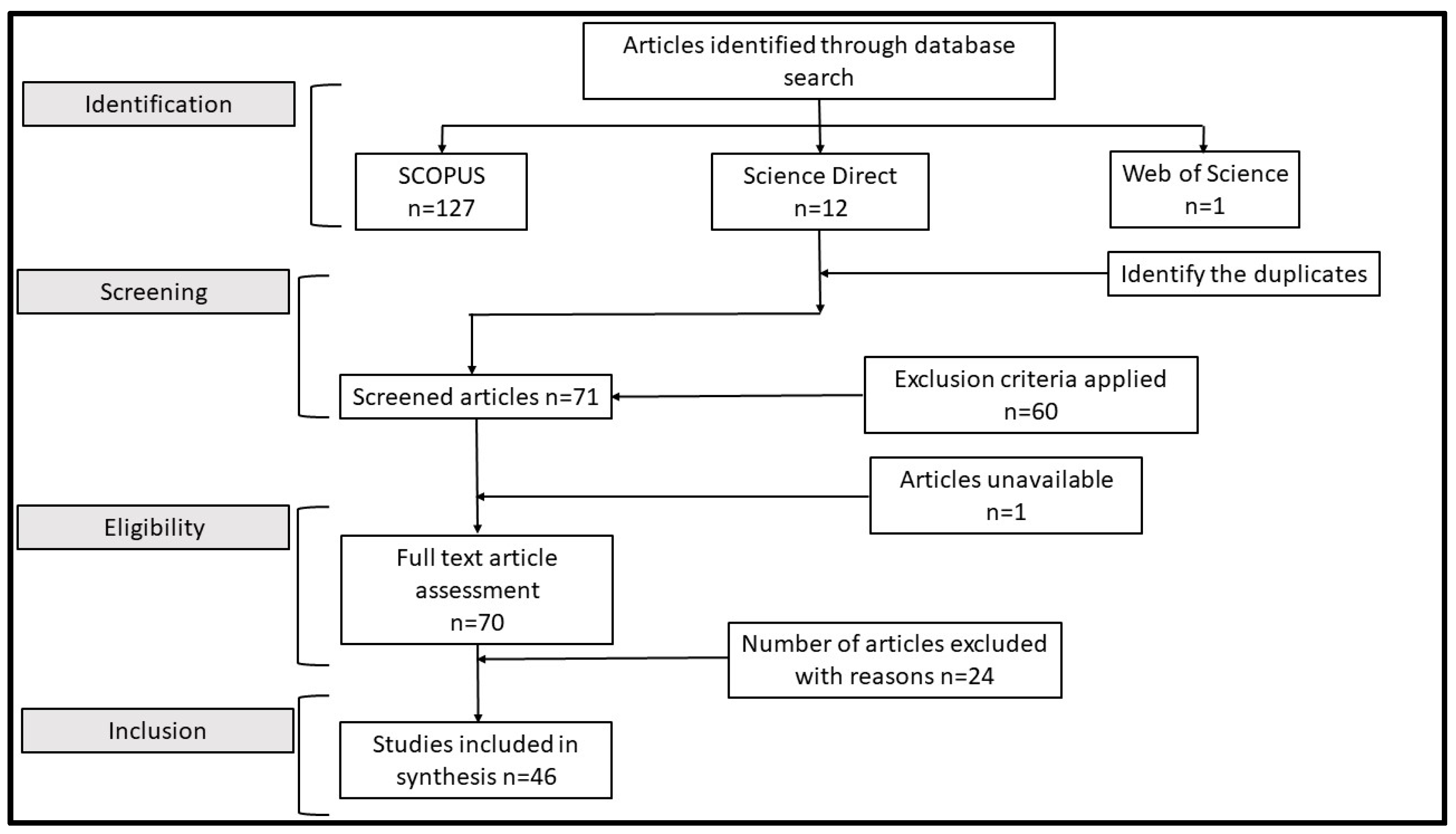
Disclaimer/Publisher’s Note: The statements, opinions and data contained in all publications are solely those of the individual author(s) and contributor(s) and not of MDPI and/or the editor(s). MDPI and/or the editor(s) disclaim responsibility for any injury to people or property resulting from any ideas, methods, instructions or products referred to in the content. |
© 2024 by the authors. Licensee MDPI, Basel, Switzerland. This article is an open access article distributed under the terms and conditions of the Creative Commons Attribution (CC BY) license (https://creativecommons.org/licenses/by/4.0/).