
Real-Time Synthetic Aperture Radar Imaging with Random Sampling Employing Scattered Power Mapping


Abstract
:1. Introduction
2. Methodology
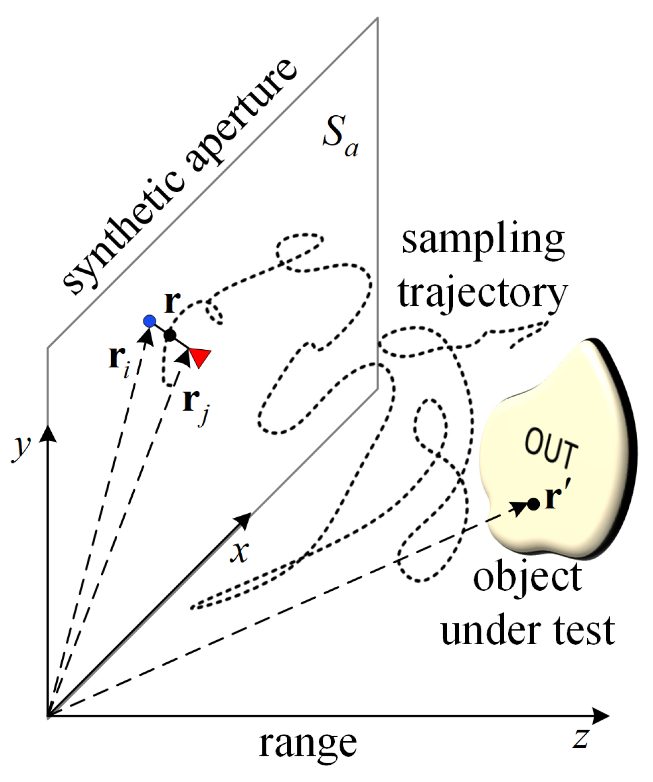
2.1. 3D Scanning
2.2. Image Reconstruction with Randomly Sampled Data Employing Scattered Power Mapping
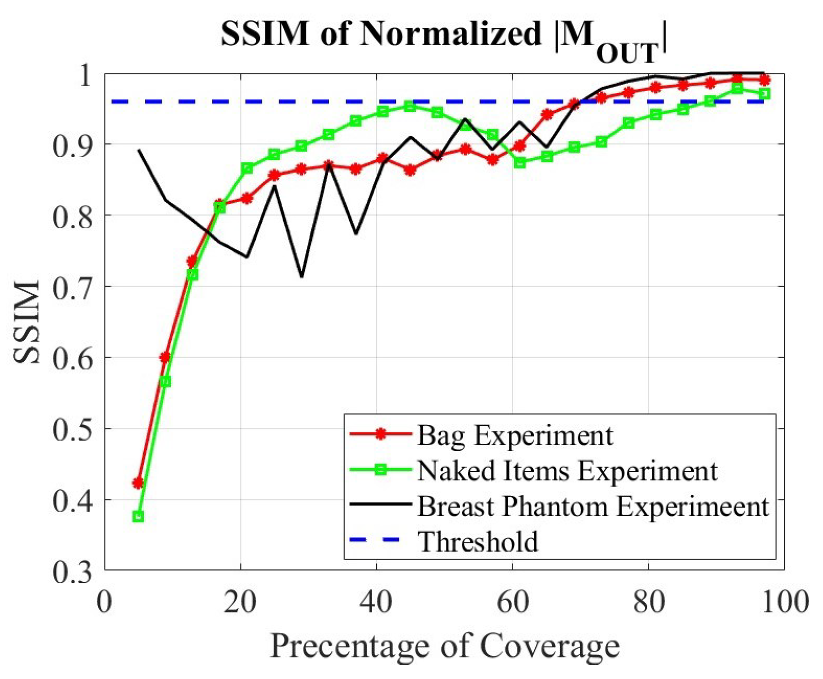
2.3. Image-Convergence Check
3. Validation Examples with Simulated Data
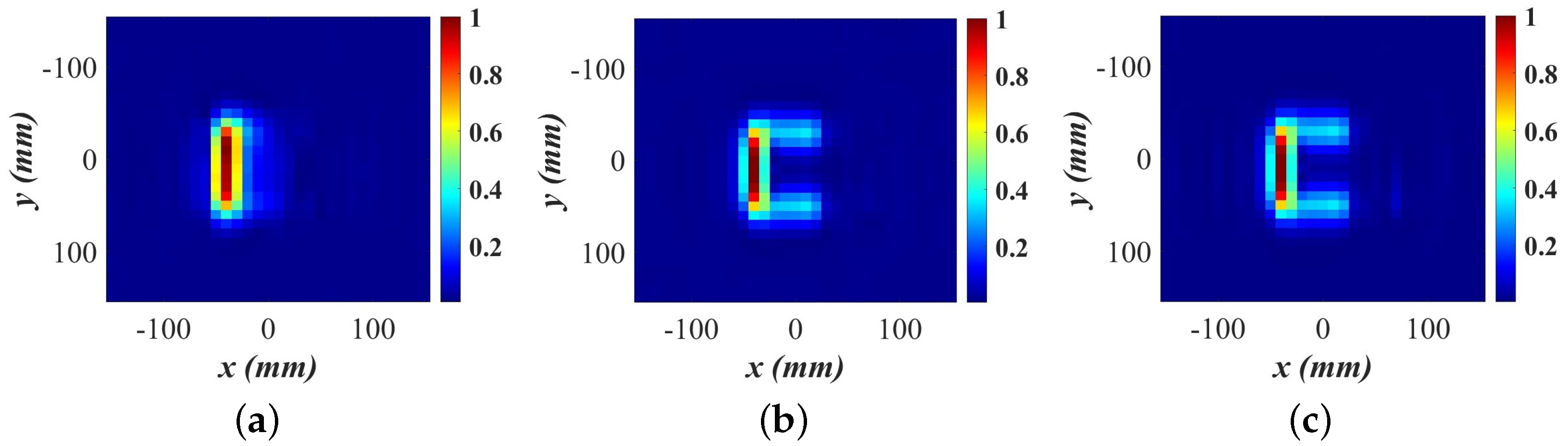
3.1. C Shape Image Reconstruction with Simulated Data
3.2. F Shape Image Reconstruction with LFM Radar Synthetic Data
4. Validation Examples with Measured Data
4.1. Compressed Breast Phantom Imaging
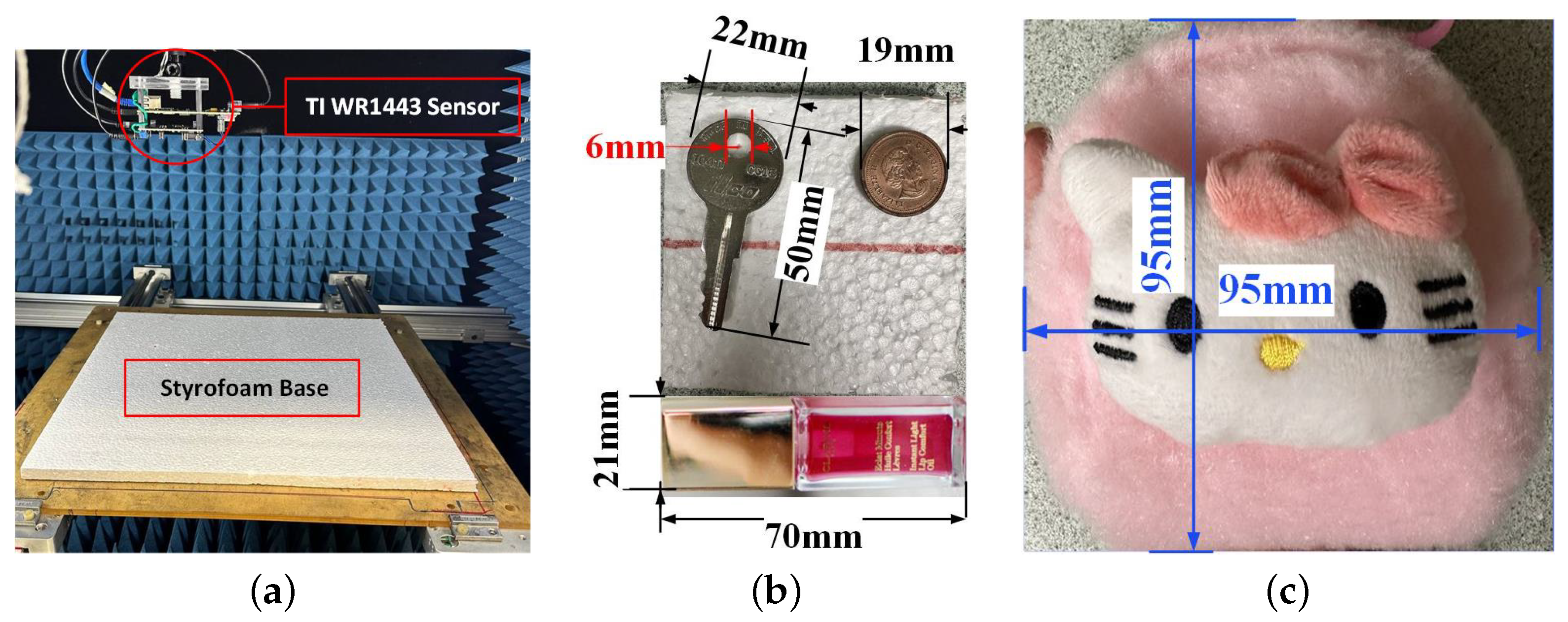
4.2. Imaging of Various Small Items with mm-Wave LFM Radar
5. Discussion
6. Conclusions and Future Work
Author Contributions
Funding
Institutional Review Board Statement
Informed Consent Statement
Data Availability Statement
Acknowledgments
Conflicts of Interest
Correction Statement
References
- Kharkovsky, S.; Case, J.; Abou-Khousa, M.; Zoughi, R.; Hepburn, F. Millimeter-wave detection of localized anomalies in the space shuttle external fuel tank insulating foam. IEEE Trans. Instrum. Meas. 2006, 55, 1250–1257. [Google Scholar] [CrossRef]
- Dvorsky, M.; Sim, S.Y.; Motes, D.T.; Watt, T.; Shah, A.; Qaseer, M.T.A.; Zoughi, R. Multistatic Ka-Band (26.5–40 GHz) Millimeter-Wave 3-D Imaging System. IEEE Trans. Instrum. Meas. 2023, 72, 1–14. [Google Scholar] [CrossRef]
- Horst, M.J.; Ghasr, M.T.; Zoughi, R. A Compact Microwave Camera Based on Chaotic Excitation Synthetic-Aperture Radar. IEEE Trans. Antennas Propag. 2019, 67, 4148–4161. [Google Scholar] [CrossRef]
- Truong, T.; Dinh, A.; Wahid, K. An Ultra-Wideband Frequency System for Non-Destructive Root Imaging. Sensors 2018, 18, 2438. [Google Scholar] [CrossRef]
- Abou-Khousa, M.A.; Rahman, M.S.U.; Donnell, K.M.; Qaseer, M.T.A. Detection of Surface Cracks in Metals Using Microwave and Millimeter-Wave Nondestructive Testing Techniques—A Review. IEEE Trans. Instrum. Meas. 2023, 72, 1–18. [Google Scholar] [CrossRef]
- Liu, C.; Zoughi, R. Adaptive Synthetic Aperture Radar (SAR) Imaging for Optimal Cross-Range Resolution and Image Quality in NDE Applications. IEEE Trans. Instrum. Meas. 2021, 70, 1–7. [Google Scholar] [CrossRef]
- Paun, M. Through-Wall Imaging Using Low-Cost Frequency-Modulated Continuous Wave Radar Sensors. Remote Sens. 2024, 16, 1426. [Google Scholar] [CrossRef]
- Zhuravlev, A.; Razevig, V.; Rogozin, A.; Chizh, M. Microwave Imaging of Concealed Objects with Linear Antenna Array and Optical Tracking of the Target for High-Performance Security Screening Systems. IEEE Trans. Microw. Theory Tech. 2023, 71, 1326–1336. [Google Scholar] [CrossRef]
- Gui, S.; Li, J.; Yang, Y.; Zuo, F.; Pi, Y. A SAR Imaging Method for Walking Human Based on mωka-FrFT-mmGLRT. IEEE Trans. Geosci. Remote Sens. 2022, 60, 1–12. [Google Scholar] [CrossRef]
- Gui, S.; Yang, Y.; Li, J.; Zuo, F.; Pi, Y. THz Radar Security Screening Method for Walking Human Torso with Multi-Angle Synthetic Aperture. IEEE Sensors J. 2021, 21, 17962–17972. [Google Scholar] [CrossRef]
- Zhuravlev, A.; Razevig, V.; Chizh, M.; Dong, G.; Hu, B. A New Method for Obtaining Radar Images of Concealed Objects in Microwave Personnel Screening Systems. IEEE Trans. Microw. Theory Tech. 2021, 69, 357–364. [Google Scholar] [CrossRef]
- Chen, X.; Yang, Q.; Wang, H.; Zeng, Y.; Deng, B. Adaptive ADMM-Based High-Quality Fast Imaging Algorithm for Short-Range MMW MIMO-SAR Systems. IEEE Trans. Antennas Propag. 2023, 71, 8925–8935. [Google Scholar] [CrossRef]
- Pang, L.; Liu, H.; Chen, Y.; Miao, J. Real-time Concealed Object Detection from Passive Millimeter Wave Images Based on the YOLOv3 Algorithm. Sensors 2020, 20, 1678. [Google Scholar] [CrossRef]
- Liang, F.; Wang, P.; Lv, H.; Bai, M.; An, Q.; Han, S.; Zhang, Y.; Wang, J. Change Detection and Enhanced Imaging of Vital Signs Based on Arc-Scanning SAR. IEEE Sensors J. 2024, 24, 8304–8313. [Google Scholar] [CrossRef]
- Owda, A.Y.; Owda, M.; Rezgui, N.D. Synthetic Aperture Radar Imaging for Burn Wounds Diagnostics. Sensors 2020, 20, 847. [Google Scholar] [CrossRef]
- Klemm, M.; Leendertz, J.A.; Gibbins, D.; Craddock, I.J.; Preece, A.; Benjamin, R. Microwave Radar-Based Differential Breast Cancer Imaging: Imaging in Homogeneous Breast Phantoms and Low Contrast Scenarios. IEEE Trans. Antennas Propag. 2010, 58, 2337–2344. [Google Scholar] [CrossRef]
- Li, H.; Zhang, H.; Kong, Y.; Zhou, C. Flexible Dual-Polarized UWB Antenna Sensors for Breast Tumor Detection. IEEE Sens. J. 2022, 22, 13648–13658. [Google Scholar] [CrossRef]
- Ghamati, M.; Taherzadeh, M.; Nabki, F.; Popović, M. Integrated Fast UWB Time-Domain Microwave Breast Screening. IEEE Trans. Instrum. Meas. 2023, 72, 1–12. [Google Scholar] [CrossRef]
- Dachena, C.; Fedeli, A.; Fanti, A.; Lodi, M.B.; Fumera, G.; Randazzo, A.; Pastorino, M. Microwave Imaging of the Neck by Means of Artificial Neural Networks for Tumor Detection. IEEE Open J. Antennas Propag. 2021, 2, 1044–1056. [Google Scholar] [CrossRef]
- Hosseinzadegan, S.; Fhager, A.; Persson, M.; Geimer, S.D.; Meaney, P.M. Discrete Dipole Approximation-Based Microwave Tomography for Fast Breast Cancer Imaging. IEEE Trans. Microw. Theory Tech. 2021, 69, 2741–2752. [Google Scholar] [CrossRef]
- Zhang, L.; Qiao, Z.; Xing, M.d.; Yang, L.; Bao, Z. A Robust Motion Compensation Approach for UAV SAR Imagery. IEEE Trans. Geosci. Remote Sens. 2012, 50, 3202–3218. [Google Scholar] [CrossRef]
- Zhang, F.; Yan, S.; Fu, Y.; Yang, W.; Zhang, W.; Yu, R. A Novel Motion Compensation Framework for Micro UAV FMCW SAR. In Proceedings of the 2023 IEEE 16th International Conference on Electronic Measurement & Instruments (ICEMI), Harbin, China, 9–11 August 2023; pp. 304–308. [Google Scholar] [CrossRef]
- Koo, V.; Chan, Y.K.; Vetharatnam, G.; Chua, M.Y.; Lim, C.H.; Lim, C.S.; Thum, C.C.; Lim, T.S.; bin Ahmad, Z.; Mahmood, K.A.; et al. A new unmanned aerial vehicle synthetic aperture radar for environmental monitoring. Prog. Electromagn. Res. 2012, 122, 245–268. [Google Scholar] [CrossRef]
- Ding, J.; Zhang, K.; Huang, X.; Xu, Z. High Frame-Rate Imaging Using Swarm of UAV-Borne Radars. IEEE Trans. Geosci. Remote Sens. 2024, 62, 1–12. [Google Scholar] [CrossRef]
- Faul, F.T.; Korthauer, D.; Eibert, T.F. Impact of Rotor Blade Rotation of UAVs on Electromagnetic Field Measurements. IEEE Trans. Instrum. Meas. 2021, 70, 1–9. [Google Scholar] [CrossRef]
- Lyu, M.; Zhao, Y.; Huang, C.; Huang, H. Unmanned Aerial Vehicles for Search and Rescue: A Survey. Remote Sens. 2023, 15, 3266. [Google Scholar] [CrossRef]
- Garcia Fernandez, M.; Alvarez Lopez, Y.; Arboleya Arboleya, A.; Gonzalez Valdes, B.; Rodriguez Vaqueiro, Y.; Las-Heras Andres, F.; Pino Garcia, A. Synthetic Aperture Radar Imaging System for Landmine Detection Using a Ground Penetrating Radar on Board a Unmanned Aerial Vehicle. IEEE Access 2018, 6, 45100–45112. [Google Scholar] [CrossRef]
- Lopez, Y.A.; Garcia-Fernandez, M.; Alvarez-Narciandi, G.; Andres, F.L.H. Unmanned Aerial Vehicle-Based Ground-Penetrating Radar Systems: A review. IEEE Geosci. Remote Sens. Mag. 2022, 10, 66–86. [Google Scholar] [CrossRef]
- Garcia-Fernandez, M.; Alvarez-Narciandi, G.; Heras, F.L.; Alvarez-Lopez, Y. Comparison of Scanning Strategies in UAV-Mounted Multichannel GPR-SAR Systems Using Antenna Arrays. IEEE J. Sel. Top. Appl. Earth Obs. Remote Sens. 2024, 7, 3571–3586. [Google Scholar] [CrossRef]
- Amiri, A.; Tong, K.; Chetty, K. Feasibility study of multi-frequency Ground Penetrating Radar for rotary UAV platforms. In Proceedings of the IET International Conference on Radar Systems (Radar 2012), Glasgow, UK, 22–25 October 2012; pp. 1–6. [Google Scholar] [CrossRef]
- Weib, M.; Ender, J. A 3D imaging radar for small unmanned airplanes—ARTINO. In Proceedings of the 2005 European Radar Conference (EURAD 2005), Paris, France, 3–4 October 2005; pp. 209–212. [Google Scholar] [CrossRef]
- Yarleque, M.A.; Alvarez, S.; Martinez, H.J. FMCW GPR radar mounted in a mini-UAV for archaeological applications: First analytical and measurement results. In Proceedings of the 2017 International Conference on Electromagnetics in Advanced Applications (ICEAA), Verona, Italy, 11–15 September 2017; pp. 1646–1648. [Google Scholar] [CrossRef]
- Ludeno, G.; Catapano, I.; Renga, A.; Vetrella, A.R.; Fasano, G.; Soldovieri, F. Assessment of a micro-UAV system for microwave tomography radar imaging. Remote Sens. Environ. 2018, 212, 90–102. [Google Scholar] [CrossRef]
- Grathwohl, A.; Arendt, B.; Grebner, T.; Waldschmidt, C. Detection of Objects Below Uneven Surfaces with a UAV-Based GPSAR. IEEE Trans. Geosci. Remote Sens. 2023, 61, 1–13. [Google Scholar] [CrossRef]
- Pierce, A. Walabot DIY can see into walls. Technol. Today 2017, 76, 8–9. [Google Scholar]
- Vayyar Imaging—Home. Available online: https://vayyar.com/ (accessed on 11 June 2024).
- The World’s Most Advanced Stud Finder. Available online: https://walabot.com/ (accessed on 11 June 2024).
- Nikolova, N.K. Introduction to Microwave Imaging; EuMA High Frequency Technologies Series; Cambridge University Press: Cambridge, UK, 2017. [Google Scholar] [CrossRef]
- Amineh, R.K.; Nikolova, N.K.; Ravan, M. Real-Time Three-Dimensional Imaging of Dielectric Bodies Using Microwave/Millimeter Wave Holography; John Wiley & Sons: Hoboken, NJ, USA, 2019. [Google Scholar]
- Sheen, D.; McMakin, D.; Hall, T. Three-dimensional millimeter-wave imaging for concealed weapon detection. IEEE Trans. Microw. Theory Tech. 2001, 49, 1581–1592. [Google Scholar] [CrossRef]
- Austin, C.D.; Ertin, E.; Moses, R.L. Sparse Signal Methods for 3-D Radar Imaging. IEEE J. Sel. Top. Signal Process. 2011, 5, 408–423. [Google Scholar] [CrossRef]
- Fessler, J.; Sutton, B. Nonuniform fast Fourier transforms using min-max interpolation. IEEE Trans. Signal Process. 2003, 51, 560–574. [Google Scholar] [CrossRef]
- Sun, D.; Pang, B.; Xing, S.; Li, Y.; Wang, X. Direct 3-D Sparse Imaging Using Non-Uniform Samples without Data Interpolation. Electronics 2020, 9, 321. [Google Scholar] [CrossRef]
- Case, J.T.; Ghasr, M.T.; Zoughi, R. Optimum 2-D Nonuniform Spatial Sampling for Microwave SAR-Based NDE Imaging Systems. IEEE Trans. Instrum. Meas. 2012, 61, 3072–3083. [Google Scholar] [CrossRef]
- Marvasti, F. Nonuniform sampling theorems for bandpass signals at or below the Nyquist density. IEEE Trans. Signal Process. 1996, 44, 572–576. [Google Scholar] [CrossRef]
- Marvasti, F. Interpolation of lowpass signals at half the Nyquist rate. In Proceedings of the 1995 International Conference on Acoustics, Speech, and Signal Processing, Detroit, MI, USA, 9–12 May 1995; Volume 2, pp. 1225–1228. [Google Scholar] [CrossRef]
- Zhou, S.; Yang, L.; Zhao, L.; Bi, G. Forward Velocity Extraction From UAV Raw SAR Data Based on Adaptive Notch Filtering. IEEE Geosci. Remote Sens. Lett. 2016, 13, 1211–1215. [Google Scholar] [CrossRef]
- Farhadi, M.; Feger, R.; Fink, J.; Wagner, T.; Stelzer, A. Combining MIMO DBF with Automotive Synthetic Aperture Radar Imaging and Phase Error Correction. IEEE Access 2024, 12, 31944–31959. [Google Scholar] [CrossRef]
- Saurer, M.M.; Hofmann, B.; Eibert, T.F. A Fully Polarimetric Multilevel Fast Spectral Domain Algorithm for 3-D Imaging with Irregular Sample Locations. IEEE Trans. Microw. Theory Tech. 2022, 70, 4231–4242. [Google Scholar] [CrossRef]
- Yegulalp, A. Fast backprojection algorithm for synthetic aperture radar. In Proceedings of the 1999 IEEE Radar Conference. Radar into the Next Millennium (Cat. No.99CH36249), Waltham, MA, USA, 22 April 1999; pp. 60–65. [Google Scholar] [CrossRef]
- Moreira, A.; Huang, Y. Airborne SAR processing of highly squinted data using a chirp scaling approach with integrated motion compensation. IEEE Trans. Geosci. Remote Sens. 1994, 32, 1029–1040. [Google Scholar] [CrossRef]
- Zhou, L.; Zhang, X.; Wang, Y.; Li, L.; Pu, L.; Shi, J.; Wei, S. Unambiguous Reconstruction for Multichannel Nonuniform Sampling SAR Signal Based on Image Fusion. IEEE Access 2020, 8, 71558–71571. [Google Scholar] [CrossRef]
- Krieger, G.; Gebert, N.; Moreira, A. Unambiguous SAR signal reconstruction from nonuniform displaced phase center sampling. IEEE Geosci. Remote Sens. Lett. 2004, 1, 260–264. [Google Scholar] [CrossRef]
- Eldar, Y.; Oppenheim, A. Filterbank reconstruction of bandlimited signals from nonuniform and generalized samples. IEEE Trans. Signal Process. 2000, 48, 2864–2875. [Google Scholar] [CrossRef]
- Lopez-Sanchez, J.; Fortuny-Guasch, J. 3-D radar imaging using range migration techniques. IEEE Trans. Antennas Propag. 2000, 48, 728–737. [Google Scholar] [CrossRef]
- Gao, Y.; Ghasr, M.T.; Zoughi, R. Effects of and Compensation for Translational Position Error in Microwave Synthetic Aperture Radar Imaging Systems. IEEE Trans. Instrum. Meas. 2020, 69, 1205–1212. [Google Scholar] [CrossRef]
- Case, J.T.; Ghasr, M.T.; Zoughi, R. Nonuniform Manual Scanning for Rapid Microwave Nondestructive Evaluation Imaging. IEEE Trans. Instrum. Meas. 2013, 62, 1250–1258. [Google Scholar] [CrossRef]
- Meng, D.; Hu, D.; Ding, C. Precise Focusing of Airborne SAR Data with Wide Apertures Large Trajectory Deviations: A Chirp Modulated Back-Projection Approach. IEEE Trans. Geosci. Remote Sens. 2015, 53, 2510–2519. [Google Scholar] [CrossRef]
- Zhang, G.; Li, C.; Wang, Z.; Hu, J.; Zheng, S.; Liu, X.; Fang, G. An Efficient Spectrum Reconstruction Algorithm for Non-Uniformly Sampled Signals and Its Application in Terahertz SAR. Remote Sens. 2023, 15, 4427. [Google Scholar] [CrossRef]
- Wu, S.; Ding, L.; Li, P.; Li, Y.; Chen, L.; Zhu, Y. Millimeter-Wave SAR Sparse Imaging with 2-D Spatially Pseudorandom Spiral-Sampling Pattern. IEEE Trans. Microw. Theory Tech. 2020, 68, 4672–4683. [Google Scholar] [CrossRef]
- Hu, S.; Molaei, A.M.; Yurduseven, O.; Meng, H.; Nilavalan, R.; Gan, L.; Chen, X. Multistatic MIMO Sparse Imaging Based on FFT and Low-Rank Matrix Recovery Techniques. IEEE Trans. Microw. Theory Tech. 2023, 71, 1285–1295. [Google Scholar] [CrossRef]
- Zhang, T.; Li, Y.; Wang, J.; Xing, M.; Guo, L.; Zhang, P. a Modified Range Model and Extended Omega-K Algorithm for High-Speed-High-Squint SAR with Curved Trajectory. IEEE Trans. Geosci. Remote Sens. 2023, 61, 1–15. [Google Scholar] [CrossRef]
- Xu, Z.; Liu, M.; Zhou, G.; Wei, Z.; Zhang, B.; Wu, Y. An Accurate Sparse SAR Imaging Method for Enhancing Region-Based Features Via Nonconvex and TV Regularization. IEEE J. Sel. Top. Appl. Earth Obs. Remote Sens. 2021, 14, 350–363. [Google Scholar] [CrossRef]
- Liu, M.; Pan, J.; Zhu, J.; Chen, Z.; Zhang, B.; Wu, Y. A Sparse SAR Imaging Method for Low-Oversampled Staggered Mode via Compound Regularization. Remote Sens. 2024, 16, 1459. [Google Scholar] [CrossRef]
- Ao, D.; Wang, R.; Hu, C.; Li, Y. A Sparse SAR Imaging Method Based on Multiple Measurement Vectors Model. Remote Sens. 2017, 9, 297. [Google Scholar] [CrossRef]
- Wang, Y.; He, Z.; Zhan, X.; Fu, Y.; Zhou, L. Three-Dimensional Sparse SAR Imaging with Generalized Lq Regularization. Remote Sens. 2022, 14, 288. [Google Scholar] [CrossRef]
- Candes, E.J.; Wakin, M.B. An Introduction To Compressive Sampling. IEEE Signal Process. Mag. 2008, 25, 21–30. [Google Scholar] [CrossRef]
- Pham, T.H.; Kim, K.H.; Hong, I.P. A Study on Millimeter Wave SAR Imaging for Non-Destructive Testing of Rebar in Reinforced Concrete. Sensors 2022, 22, 30. [Google Scholar] [CrossRef]
- Pu, W.; Huang, Y.; Wu, J.; Yang, H.; Yang, J. Fast Compressive Sensing-Based SAR Imaging Integrated with Motion Compensation. IEEE Access 2019, 7, 53284–53295. [Google Scholar] [CrossRef]
- Yang, J.; Jin, T.; Xiao, C.; Huang, X. Compressed Sensing Radar Imaging: Fundamentals, Challenges, and Advances. Sensors 2019, 19, 3100. [Google Scholar] [CrossRef]
- Kang, M.S.; Baek, J.M. SAR Image Reconstruction via Incremental Imaging with Compressive Sensing. IEEE Trans. Aerosp. Electron. Syst. 2023, 59, 4450–4463. [Google Scholar] [CrossRef]
- Dong, B.; Li, G.; Zhang, Q. High-Resolution and Wide-Swath Imaging of Spaceborne SAR via Random PRF Variation Constrained by the Coverage Diagram. IEEE Trans. Geosci. Remote Sens. 2022, 60, 1–16. [Google Scholar] [CrossRef]
- Abo-Zahhad, M.M.; Hussein, A.I.; Mohamed, A.M. Compressive sensing algorithms for signal processing applications: A survey. Int. J. Commun. Netw. Syst. Sci. 2015, 8, 197–216. [Google Scholar]
- Bernhardt, S.; Boyer, R.; Marcos, S.; Larzabal, P. Compressed Sensing with Basis Mismatch: Performance Bounds and Sparse-Based Estimator. IEEE Trans. Signal Process. 2016, 64, 3483–3494. [Google Scholar] [CrossRef]
- Tu, S.; McCombe, J.J.; Shumakov, D.S.; Nikolova, N.K. Fast quantitative microwave imaging with resolvent kernel extracted from measurements. Inverse Probl. 2015, 31, 045007. [Google Scholar] [CrossRef]
- Shumakov, D.S.; Nikolova, N.K. Fast Quantitative Microwave Imaging with Scattered-Power Maps. IEEE Trans. Microw. Theory Tech. 2018, 66, 439–449. [Google Scholar] [CrossRef]
- Kazemivala, R.; Tajik, D.; Nikolova, N.K. Simultaneous Use of the Born and Rytov Approximations in Real-Time Imaging with Fourier-Space Scattered Power Mapping. IEEE Trans. Microw. Theory Tech. 2022, 70, 2904–2920. [Google Scholar] [CrossRef]
- Kazemivala, R.; Pitcher, A.D.; Nguyen, J.; Nikolova, N.K. Real-Time Millimeter-wave Imaging with Linear Frequency Modulation Radar and Scattered Power Mapping. IEEE Trans. Microw. Theory Tech. 2024; Early Access. [Google Scholar] [CrossRef]
- Liu, L.; Trehan, A.C.; Nikolova, N.K. Near-field detection at microwave frequencies based on self-adjoint response sensitivity analysis. Inverse Probl. 2010, 26, 105001. [Google Scholar] [CrossRef]
- Liu, C.; Qaseer, M.T.A.; Zoughi, R. Influence of Antenna Pattern on Synthetic Aperture Radar Resolution for NDE Applications. IEEE Trans. Instrum. Meas. 2021, 70, 8000911. [Google Scholar] [CrossRef]
- Amineh, R.K.; McCombe, J.; Nikolova, N.K. Microwave Holographic Imaging Using the Antenna Phaseless Radiation Pattern. IEEE Antennas Wirel. Propag. Lett. 2012, 11, 1529–1532. [Google Scholar] [CrossRef]
- Meng, Y.; Lin, C.; Zang, J.; Qing, A.; Nikolova, N.K. General Theory of Holographic Inversion with Linear Frequency Modulation Radar and its Application to Whole-Body Security Scanning. IEEE Trans. Microw. Theory Tech. 2020, 68, 4694–4705. [Google Scholar] [CrossRef]
- Gao, J.; Deng, B.; Qin, Y.; Wang, H.; Li, X. An Efficient Algorithm for MIMO Cylindrical Millimeter-Wave Holographic 3-D Imaging. IEEE Trans. Microw. Theory Tech. 2018, 66, 5065–5074. [Google Scholar] [CrossRef]
- Tajik, D.; Kazemivala, R.; Nguyen, J.; Nikolova, N.K. Accurate Range Migration for Fast Quantitative Fourier-Based Image Reconstruction with Monostatic Radar. IEEE Trans. Microw. Theory Tech. 2022, 70, 4273–4283. [Google Scholar] [CrossRef]
- Cheng, Q.; Alomainy, A.; Hao, Y. Near-Field Millimeter-Wave Phased Array Imaging with Compressive Sensing. IEEE Access 2017, 5, 18975–18986. [Google Scholar] [CrossRef]
- Beaverstone, A.S.; Shumakov, D.S.; Nikolova, N.K. Frequency-Domain Integral Equations of Scattering for Complex Scalar Responses. IEEE Trans. Microw. Theory Tech. 2017, 65, 1120–1132. [Google Scholar] [CrossRef]
- Pozar, D.M. Microwave Engineering, 4th ed.; John Wiley & Sons: Hoboken, NJ, USA, 2012. [Google Scholar]
- Wang, Y.; Abbosh, A.M.; Henin, B.; Nguyen, P.T. Synthetic Bandwidth Radar for Ultra-Wideband Microwave Imaging Systems. IEEE Trans. Antennas Propag. 2014, 62, 698–705. [Google Scholar] [CrossRef]
- Yi, L.; Kaname, R.; Mizuno, R.; Li, Y.; Fujita, M.; Ito, H.; Nagatsuma, T. Ultra-Wideband Frequency Modulated Continuous Wave Photonic Radar System for Three-Dimensional Terahertz Synthetic Aperture Radar Imaging. J. Light. Technol. 2022, 40, 6719–6728. [Google Scholar] [CrossRef]
- Özdemir, C.; Demirci, Ş.; Yiğit, E.; Yilmaz, B. A Review on Migration Methods in B-Scan Ground Penetrating Radar Imaging. Math. Probl. Eng. 2014, 2014, 280738. [Google Scholar] [CrossRef]
- Amineh, R.K.; Khalatpour, A.; Xu, H.; Baskharoun, Y.; Nikolova, N.K. Three-dimensional near-field microwave holography for tissue imaging. J. Biomed. Imaging 2012, 2012, 5. [Google Scholar] [CrossRef]
- Amineh, R.K.; McCombe, J.J.; Khalatpour, A.; Nikolova, N.K. Microwave Holography Using Point-Spread Functions Measured with Calibration Objects. IEEE Trans. Instrum. Meas. 2015, 64, 403–417. [Google Scholar] [CrossRef]
- Altair Feko, Version 2018; Altair Engineering Inc.: Troy, MI, USA, 2018.
- MATLAB, Version R2022b; The MathWorks Inc.: Natick, MA, USA, 2022.
- Tajik, D.; Kazemivala, R.; Nikolova, N.K. Real-Time Imaging with Simultaneous Use of Born and Rytov Approximations in Quantitative Microwave Holography. IEEE Trans. Microw. Theory Tech. 2022, 70, 1896–1909. [Google Scholar] [CrossRef]
- Balanis, C.K. Antenna Theory Analysis and Design; John Wiley & Sons, Inc.: Hoboken, NJ, USA, 1997. [Google Scholar]
- Shahmirzadi, N.V.; Tyagi, V.; Nguyen, J.; Kazemivala, R.; Nikolova, N.K.; Chen, C.H. Planar Array of UWB Active Slot Antennas for Microwave Imaging of the Breast. IEEE Trans. Antennas Propag. 2023, 71, 2946–2957. [Google Scholar] [CrossRef]
- Tajik, D.; Pitcher, A.D.; Nikolova, N.K. Comparative study of the Rytov and Born approximations in quantitative microwave holography. Prog. Electromagn. Res. B 2017, 79, 1–19. [Google Scholar] [CrossRef]
- Texas Instruments. IWR1443BOOST Evaluation Module mmWave Sensing Solution; Texas Instruments: Dallas, TX, USA, 2020. [Google Scholar]
- Texas Instruments. DCA1000EVM Real-Time Data-Capture Adapter for Radar Sensing Evaluation Module; Texas Instruments: Dallas, TX, USA, 2019. [Google Scholar]
- Wen, M.; Houlihan, J. Application of the non-uniform Fourier transform to non-uniformly sampled Fourier transform spectrometers. Opt. Commun. 2023, 540, 129491. [Google Scholar]
- Pitcher, A.D.; Baard, C.W.; Georgiev, M.S.; Nikolova, N.K. Ultra-wideband equivalent-time sampling receiver: Limitations and performance analysis. IEEE Trans. Instrum. Meas. 2024; submitted. [Google Scholar]


| Material (Structure) | ||
|---|---|---|
| Carbon–rubber sheet (averaged breast tissue) | 9.6 | 3.82 |
| Silicone–rubber sheet (averaged skin tissue) | 19.36 | 14 |
| Embedding/matching medium | 11.3 | 2.59 |
| Tumour simulant | 64.11 | 22.32 |
| Fibroglandular tissue simulant | 17.61 | 7.89 |
| Scattering probe (PSF) | 43.7 | 0 |
Disclaimer/Publisher’s Note: The statements, opinions and data contained in all publications are solely those of the individual author(s) and contributor(s) and not of MDPI and/or the editor(s). MDPI and/or the editor(s) disclaim responsibility for any injury to people or property resulting from any ideas, methods, instructions or products referred to in the content. |
© 2024 by the authors. Licensee MDPI, Basel, Switzerland. This article is an open access article distributed under the terms and conditions of the Creative Commons Attribution (CC BY) license (https://creativecommons.org/licenses/by/4.0/).
Share and Cite
Kazemivala, R.; Nikolova, N.K. Real-Time Synthetic Aperture Radar Imaging with Random Sampling Employing Scattered Power Mapping. Sensors 2024, 24, 3849. https://doi.org/10.3390/s24123849
Kazemivala R, Nikolova NK. Real-Time Synthetic Aperture Radar Imaging with Random Sampling Employing Scattered Power Mapping. Sensors. 2024; 24(12):3849. https://doi.org/10.3390/s24123849
Chicago/Turabian StyleKazemivala, Romina, and Natalia K. Nikolova. 2024. "Real-Time Synthetic Aperture Radar Imaging with Random Sampling Employing Scattered Power Mapping" Sensors 24, no. 12: 3849. https://doi.org/10.3390/s24123849
APA StyleKazemivala, R., & Nikolova, N. K. (2024). Real-Time Synthetic Aperture Radar Imaging with Random Sampling Employing Scattered Power Mapping. Sensors, 24(12), 3849. https://doi.org/10.3390/s24123849