Article

Performance Assessment of Two Low-Cost PM2.5 and PM10 Monitoring Networks in the Padana Plain (Italy)

1
National Research Council, Institute of Bioecomony (CNR-IBE), Via Caproni 8, 50145 Firenze, Italy
2
National Research Council, Institute of Polar Sciences (CNR-ISP), Via P. Gobetti 101, 40129 Bologna, Italy
*
Author to whom correspondence should be addressed.
Sensors 2024, 24(12), 3946; https://doi.org/10.3390/s24123946
Submission received: 10 May 2024 / Revised: 10 June 2024 / Accepted: 16 June 2024 / Published: 18 June 2024
(This article belongs to the Special Issue Feature Papers in Remote Sensors 2024)

Abstract

:
Two low-cost (LC) monitoring networks, PurpleAir (instrumented by Plantower PMS5003 sensors) and AirQino (Novasense SDS011), were assessed in monitoring PM2.5 and PM10 daily concentrations in the Padana Plain (Northern Italy). A total of 19 LC stations for PM2.5 and 20 for PM10 concentrations were compared vs. regulatory-grade stations during a full “heating season” (15 October 2022–15 April 2023). Both LC sensor networks showed higher accuracy in fitting the magnitude of PM10 than PM2.5 reference observations, while lower accuracy was shown in terms of RMSE, MAE and R2. AirQino stations under-estimated both PM2.5 and PM10 reference concentrations (MB = −4.8 and −2.9 μg/m3, respectively), while PurpleAir stations over-estimated PM2.5 concentrations (MB = +5.4 μg/m3) and slightly under-estimated PM10 concentrations (MB = −0.4 μg/m3). PurpleAir stations were finer than AirQino at capturing the time variation of both PM2.5 and PM10 daily concentrations (R2 = 0.68–0.75 vs. 0.59–0.61). LC sensors from both monitoring networks failed to capture the magnitude and dynamics of the PM2.5/PM10 ratio, confirming their well-known issues in correctly discriminating the size of individual particles. These findings suggest the need for further efforts in the implementation of mass conversion algorithms within LC units to improve the tuning of PM2.5 vs. PM10 outputs.

1. Introduction

According to the latest World Health Organization (WHO) statistics, 99% of the world’s population is living in places where air pollution levels exceed the WHO guideline limits, with 4.2 million premature deaths estimated worldwide [1]. In Europe, despite ongoing air quality improvements, air pollution is the greatest environmental health risk, causing cardiovascular and respiratory diseases, and preventable deaths [2]. Here, in 2021, 97% (76%) of the urban population was exposed to concentrations of PM2.5 (PM10) above the WHO limits [2]. The Padana Plain (Northern Italy) is one of the most polluted areas in Europe, particularly in terms of PM concentrations [3]. In 2022, PM10 concentrations in the Padana Plain were second only to those in the Balkan countries and in some industrial sites in Spain [4]. The number of annual exceedances of the PM10 daily limit value (50 μg/m3), stated by the EU Directive 2008/50/EC, reached up to 108 days, only being surpassed by that in the former Yugoslavia countries. In 2022, an average of 39.4 annual exceedances per station was recorded in the Padana Plain [4], which is higher than the maximum permitted value of 35. In Italy, air quality monitoring is officially regulated by the environmental protection agencies of each region (ARPAs), which measure PM2.5 and PM10 concentrations at daily resolution. This results in a significant knowledge gap on particulate matter (PM) temporal dynamics occurring during the day, which is critical if considering the severe PM conditions affecting the Padana Plain, particularly during the winter months [5]. This knowledge gap can be effectively filled by using low-cost (LC) sensors.
LC sensor technology has shown dramatic advances in air quality monitoring since the very first prototype developed by Bart et al. [6]. LC air pollution sensors have exhibited across the years an increasing ability to collect accurate, real-time, high spatial and temporal resolution measurements, which has favoured their development worldwide [7]. LC air quality networks are able to detect information on air pollution, temporal trends, hotspots and possibly source apportionment, that traditional (sparser) networks are unable to detect [8]. This has led to a change in air quality monitoring paradigm, as it is no longer exclusive to government organizations [9]. Current air quality legislation, on the other hand, is very inclusive towards LC sensors. In Europe, for example, the EU Directive 2008/50/EC officially incorporates LC monitors, assigning them a different regime than reference monitors, so that a lower accuracy is required to their measurements (called “indicative” rather than “regulatory”). Whereas in measuring PM concentrations, regulatory instruments typically use the gravimetric method, and LC sensors use indirect optical methods based on light scattering by particles [10]. Nephelometers and optical particle counters are the most commonly used LC sensors. The latter directly count particles according to their size, while nephelometers estimate particle density and convert it into particle mass [11]. In any case, the light-scattering approach is sensitive to variations in particle properties such as size distribution, shape and composition [12]. Increases in ambient humidity can affect hygroscopic growth of particles, and thus their light-scattering coefficient, so that the mass reported by optical sensors may be biased [13]. Therefore, the need to perform field calibration/validation of LC sensors by comparing their measurements to those from co-located regulatory stations is recommended when dealing with LC air sensor applications [7].
Over the last few years, PM measurements from several LC monitoring networks worldwide were made publicly available [14]. These networks provide geographic coverage extending from country-(e.g., Village Green, OpenSense) to continent (e.g., Citi-Sense, Smartcitizen) up to a global level (e.g., AirVisual, PurpleAir) [9]. Since most of such LC sensors only rely on calibration performed at manufacturer level (factory calibration), their pre/post-deployment evaluation vs. regulatory monitors is imperative [15]. Several worldwide performance evaluations of PM monitoring LC sensors under different real-world field conditions were performed over the years (e.g., [16]). Typically, LC units were tested vs. co-located (or at most, 1 km away) at reference stations, whereas in many practical applications, they were deployed in areas without a nearby reference system [17]. This is a serious issue, particularly in heavily PM-polluted areas, where it is instrumental to know the spatial representativeness of LC measurements and related citizen exposure.
The present study aims to bridge this gap by assessing the performance of LC sensors in monitoring PM2.5 and PM10 concentrations over a crucial hotspot such as the Padana Plain. LC sensors were assessed against various ARPA reference stations located nearby. Using reference PM2.5 and PM10 daily concentrations during the “heating season” that concurs with the most acute PM pollution episodes, two LC monitoring networks have been assessed and compared: (i) the well-established PurpleAir (https://www.purpleair.com, accessed on 16 April 2024); (ii) the newly emerging AirQino (https://www.airqino.it/en, accessed on 16 April 2024). The meaningfulness of this comparison is enhanced by the fact that these two networks are equipped with sensors built by different manufacturers. Finally, the advantages and the limitations of using LC sensor network data to improve the spatial and temporal scale of reference stations are discussed.

2. Materials and Methods
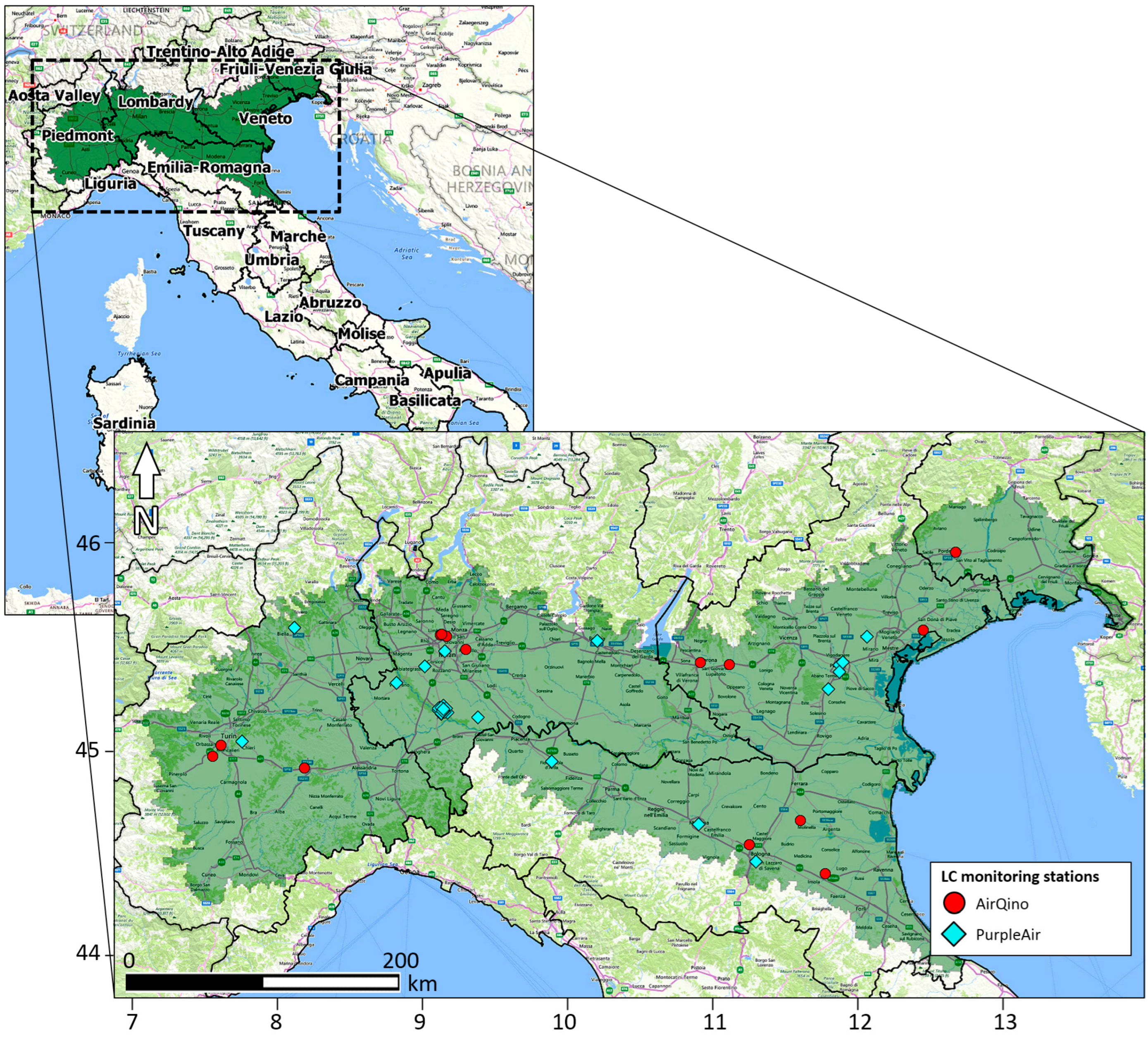
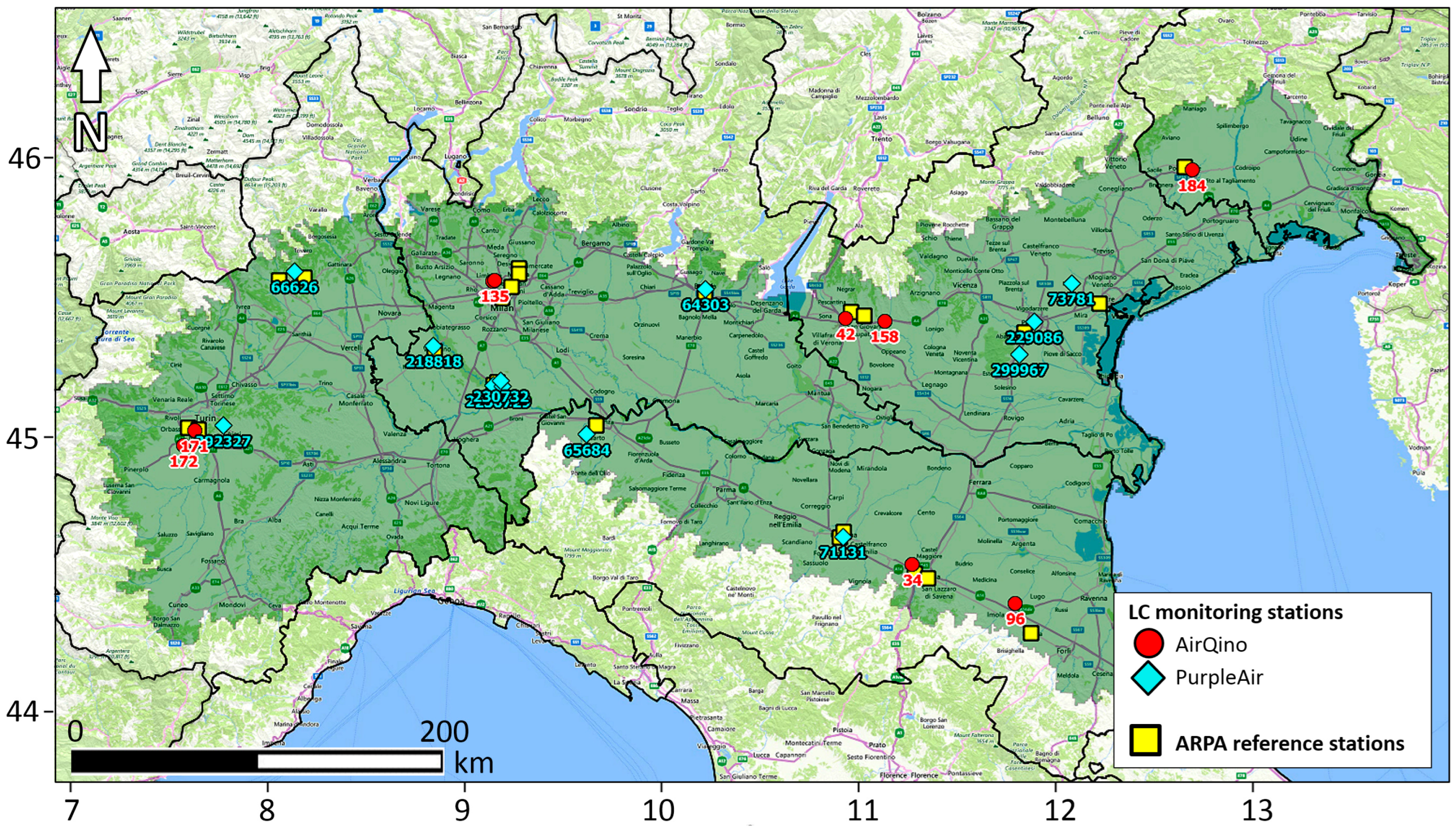
2.1. Study Area

Located in northern Italy, the Padana Plain is a morphologically and hydrographically unitary region, largely made up by the Po river valley, and limited to the N by the Alps and to the S by the Northern Apennines (Figure 1).
The Padana Plain includes five regions: Piedmont, Lombardy, Emilia-Romagna, Veneto, and Friuli-Venezia Giulia. Providing an overall share of the gross domestic product (GDP) of 50.8% [18], the Padana Plain represents a fundamental economical asset to the country. With a surface area of 49,835 m2 (16.5% of the national territory), it is home to 19,208 million inhabitants, approximately one third (32.6%) of the entire countrywide population [19]. The urbanized surface area (6885 km2) is equal to 33.9% of the national one, while population density (385.43 inhab./m2) is almost double the Italian average.
The Padana Plain is a macro-region characterized by strong (often 2 or more times higher than national average) rates of the following: (i) anthropization; (ii) industrialization; (iii) road traffic; (iv) use of biomass heating systems; (v) agricultural and livestock activities. All these drivers result in large emissions of both primary PM and secondary PM precursors such as NOx and NH3. The area is also characterized by strongly adverse meteorological conditions [20]. Particularly during colder months, the Alps and Apennines chains surrounding the region act as natural obstacles to winds and convective motions. This results in frequent wind calms and thermal inversion both at nighttime and daytime that cause the buildup and ageing of the intense emissions affecting the area [21].

2.2. Data

2.2.1. PurpleAir Low-Cost Sensors

PurpleAir (https://www.purpleair.com, accessed on 16 April 2024) is an LC sensor-based PM monitoring network started in 2015 [22], which to date has more than 10,000 monitors deployed worldwide [23]. PurpleAir is based on the PA-II unit, which contains two Plantower PMS5003 sensors (Plantower, Beijing, China) providing real-time PM measurements, units’ inner pressure, temperature, humidity and a microcontroller to communicate with the two PMS5003 sensors and with the PurpleAir server [17]. The two PMS5003 sensors provide two sets of PM readings: (i) particle number, and (ii) mass concentration [14]. These sensors are based on the light-scattering principle, with a photodiode detector converting the scattered light to a voltage pulse. The number of pulses is then converted to the number of particles in sizes of 0.3, 0.5, 1.0, 2.5, 5.0 and 10 μm [17]. A complex mass conversion algorithm—not available to the public—is applied to convert the particle counts to PM1.0, PM2.5 and PM10 mass concentrations [23]. Noteworthy, Plantower PMS5003 sensors are factory calibrated using ambient aerosol across several cities in China [13].
Over the last few years, several studies have assessed the performance of PurpleAir PA-II sensors, particularly in the US, such as in Utah [24], Pennsylvania [13,25], Colorado [10,17], Washington [14] and California [22,23,26]. Further works have also been carried out in Canada [12], China [27], Greece [28] and Africa [29].
In the present study, PM2.5 and PM10 observations from PurpleAir PA-II sensors have been downloaded from OpenAQ (https://openaq.org, accessed on 16 April 2024). OpenAQ is an open-source platform that integrates air quality data publicly released by ground-based monitors around the world as divided into reference-grade stations and LC sensors [30]. Overall, PurpleAir includes 32 LC PM2.5 and PM10 monitoring stations in the Padana Plain (Figure 1). A subset of these PurpleAir stations have been used in the present study; their location is shown in Figure 2, while their characteristics are presented in Table 1.

2.2.2. AirQino Low-Cost Sensors

AirQino (https://www.airqino.it/en, accessed on 16 April 2024) is an LC sensor-based air quality monitoring platform developed by CNR IBE [31]. The unit was conceived, created and implemented within national and international smart cities projects and device development started in 2014 [32,33]. The AirQino network currently consists of about 400 monitors mainly deployed in North and Central Italy (https://map.airqino.it, accessed on 16 April 2024). The unit is equipped with a modular set of industrial LC and high-resolution sensors aimed to collect gaseous pollutants (CO, NO2, O3), particulate matter (PM2.5 and PM10), CO2 and environmental parameters (noise, air temperature and relative humidity). The PM2.5 and PM10 sensors are based on the Novasense SDS011 detector (Nova Fitness, Jinan, China), based on the laser-scattering principle. The AirQino waterproof case was designed to minimize interference with reactive gases such as NO2 and O3; a small brushless fan creates a depression inside the box that attracts air from the inlet window. All sensors are placed beside the inlet window to reduce the contamination of fresh air inside the box (Figure S1). A microcontroller was designed and integrated into the sensor board to acquire, analyze and transmit all data through a GPRS 475G modem unit. Each device transmits geolocalized data to a central web server collecting records at high temporal and spatial resolution. Through a GIS engine and a web application, the data can be displayed, queried and analyzed in real time. The web platform integrates an SQL database and a web interface, while several APIs were developed to download data, either raw or calibrated, in Json or .csv format.
As detailed in the Supplementary Material of [34], the AirQino-integrated PM sensors were subject to various calibration and validation processes in recent years in central Italy [35,36]. The units were also tested in opposite extreme environments such as the Arctic region [37] and the Sub-Saharan Africa [34], thus proving capable of covering a full spectrum of climatic conditions and PM concentrations. Overall, a total of 14 LC PM2.5 and PM10 monitoring stations are operating in the Padana Plain (Figure 1). The location of AirQino stations used in the present study is shown in Figure 2, while their characteristics are reported in Table 1.

2.2.3. ARPA Reference Stations

PM2.5 and PM10 reference observations have been retrieved from the ARPAs operating for each region. Data have been directly downloaded from the following websites (all accessed on 16 April 2024): https://aria.ambiente.piemonte.it/qualita-aria/dati (Piedmont region); https://www.arpalombardia.it/temi-ambientali/aria/form-richiesta-dati-stazioni-fisse (Lombardy); https://www.arpa.fvg.it/temi/temi/aria/sezioni-principali/download-indicatori-e-dati-aria/indicatori-giornalieri-qualita-aria/ (Friuli Venezia Giulia); https://sdati-test.datamb.it/arex (Emilia-Romagna). As for the Veneto region, PM data have been received upon request from local ARPA. PM monitoring was performed by each regional ARPA using a dual-channel filter-based gravimetric sampling method. The location of the ARPA stations used for assessing the LC stations is shown in Figure 2. Their detailed characteristics, along with the pairing with each LC station, are presented in Table S1 (PM2.5) and Table S2 (PM10 concentrations).

2.3. Methods

PM2.5 and PM10 concentrations were collected at hourly resolution by the LC stations and then averaged to daily values to match the resolution of ARPA data. Pairing of LC stations with ARPA stations was based on the following criteria: (i) availability of PM2.5 and/or PM10 data; (ii) geographic proximity (at most within 15 km); (iii) similarity in type; (iv) a minimum of 50% concurrently available data. This resulted in the LC vs. ARPA pairing reported in Table 1 and detailed in Table S1 (PM2.5) and Table S2 (PM10 sensors). To ensure robustness of the assessment process, the monitoring campaign—consistently with [38]—focused on the colder months, i.e., the “heating season” when biomass and wood combustion for heating contributed as an additional emission source to PM concentrations. According to the Italian regulations (DPR no. 412 of 26 August 1993), in the Padana Plain, a maximum 14 h of heating usage is allowed per day during the period from 15 October to 15 April Therefore, the 15 October 2022–15 April 2023 period was selected for the current study. It was also chosen because the climatic conditions in the region trigger the maximum PM levels. An outlier removal procedure based on the interquartile (IQR) range method was applied to all datasets, i.e., removing values below (above) the first (third) quartile minus (plus) 1.5 times the IQR range.
A descriptive statistical analysis of LC and ARPA time series, including 95% confidence interval of the mean, was performed. The following statistical scores were used to assess the LC observations: mean bias (MB), linear regression’s slope and intercept, mean absolute error (MAE), root mean squared error (RMSE), coefficient of determination (R2) and correlation coefficient (r). An F test was also performed to calculate the significance level of LC observations variance with respect to ARPA observations. To evaluate performance of LC sensors in monitoring PM2.5 daily concentrations vs. regulatory monitors, the target values recommended by the United States Environmental Protection Agency (US EPA) for the ‘‘base’’ testing [39] were considered. Indeed, comparison with these target values was intended as indicative rather than stringent. Since the regulatory stations were not co-located, a field assessment—rather than a proper field validation—was performed in the study. The target values for PM2.5 sensors are detailed in Table S3.
The “R-stat” environment vs. 4.3.1 [40] was used to perform all computations. The following packages integrated in “R-stat” (and functions implemented therein) were used: “pastecs” [41] for the descriptive statistical analysis (function “stat.desc”); “Metrics” [42] to calculate the statistical scores (functions “bias”, “mae”, “rmse”); the R Stats Package [43] to calculate other metrics (“sd”, “cor”), the linear regression (“lm”) and F test (“var.test”); the R Graphics Package [44] to plot boxplots (“boxplot”) and time series (“plot”); “ggplot2” [45] to draw the scatter plots (“ggplot”); “OpenAir” [46] to plot the Taylor diagrams [47] (“TaylorDiagram”). Other functions included in the R Base Package such as “mean”, “summary” and “apply” were used.

3. Results

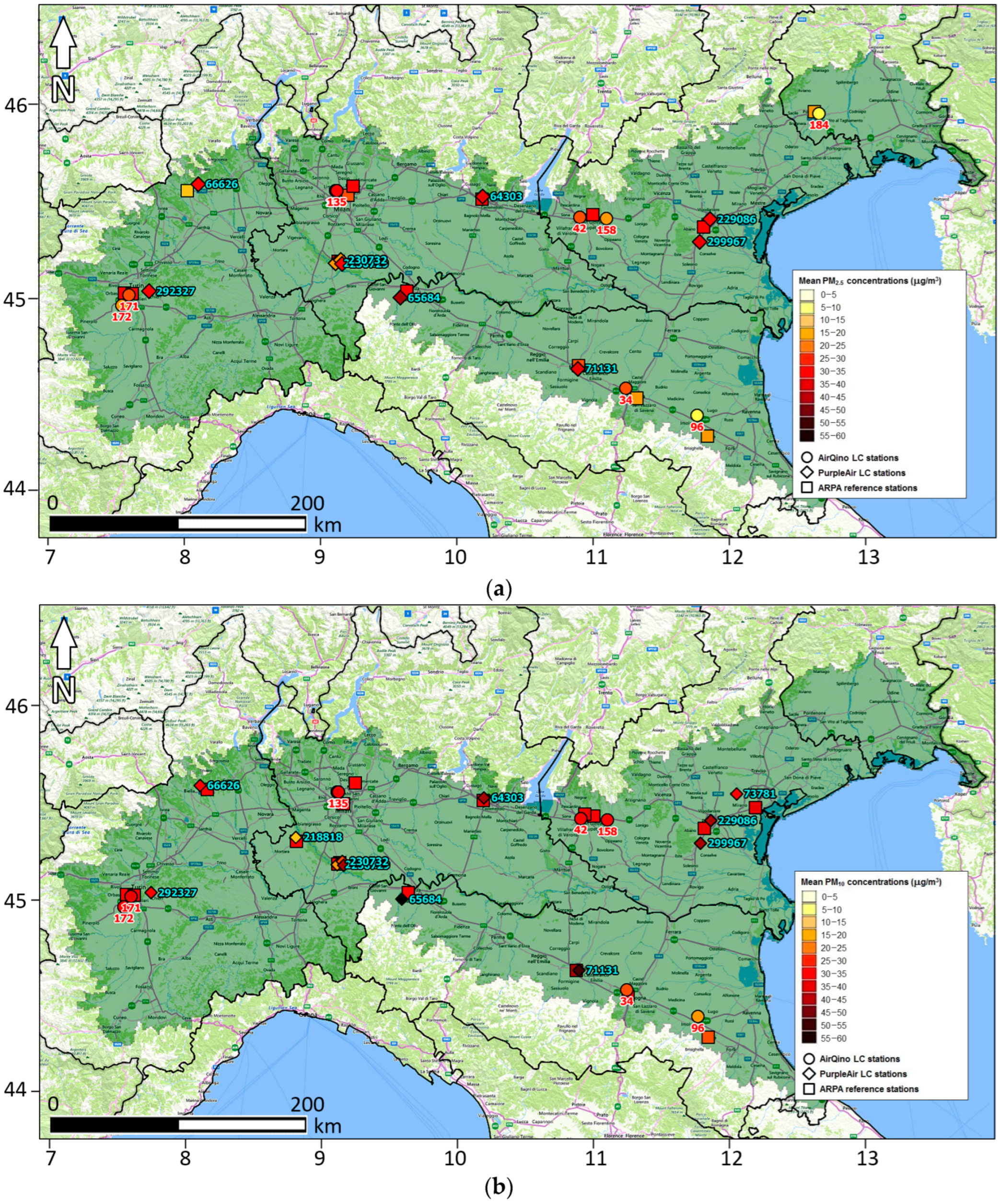
3.1. PM2.5 and PM10 Observed Concentrations

Depending on availability of ARPA stations complying with the pairing criteria set in Section 2.3, a total of 19 LC stations (9 AirQino and 10 PurpleAir) were assessed for PM2.5 monitoring, while 20 LC stations (8 AirQino and 12 PurpleAir) were assessed for PM10 monitoring. Overall, ARPA stations were located at an average distance of about 6 km from LC stations, in the range of 1.340 ÷ 13.500 km for PM2.5 concentrations (Table S1), and 0.330 ÷ 13.650 km for PM10 concentrations (Table S2). The basic statistics of PM2.5 and PM10 daily concentrations measured by all LC stations compared to the corresponding ARPA stations are summarized, respectively, in Table 2 and Table 3.
ARPA reference stations paired to the AirQino stations return a lower overall mean value of PM2.5 daily concentrations than those paired to the PurpleAir stations (22.5 vs. 26.4 μg/m3, Table 2), thus being located in environments affected by lower pollution levels. AirQino stations overall under-estimate ARPA PM2.5 observations (17.8 vs. 22.5 μg/m3), while PurpleAir stations over-estimate them (30.5 vs. 26.4 μg/m3). Conversely, both AirQino and PurpleAir stations overall under-estimate ARPA PM10 daily concentrations (31.2 vs. 34.3 μg/m3 the former, 34.5 vs. 36.8 μg/m3 the latter, Table 3).
In Table S4, the statistics of PM2.5/PM10 daily concentration ratios measured by the LC and ARPA stations are also reported. ARPA stations paired to the AirQino stations lie in areas affected by a lower amount of fine particles than those paired to the PurpleAir stations (mean ratio of 0.67 vs. 0.72). The ARPA PM2.5/PM10 ratio is generally under-estimated by the former (0.57 vs. 0.67), while over-estimated by the latter (0.85 vs. 0.72).
Figure 3 shows the map of PM2.5 and PM10 daily concentrations averaged over the full period at each LC station as compared to the corresponding ARPA stations.
AirQino stations reproduce ARPA PM2.5 observations quite well (Figure 3a), with the highest discrepancies (percentage under-estimations at worst between 40 and 60%) occurring in the eastern part of the study area (station IDs 96 and 184). PurpleAir stations are slightly finer overall than AirQino stations, though locally exhibiting higher discrepancies (percentage over-estimations at worst between 60 and 100%) occurring inland throughout the domain (IDs 65684, 66626 and 71131).
AirQino stations are particularly reliable in monitoring PM10 daily concentrations (Figure 3b); they systematically under-estimate reference observations, though exhibiting a percentage bias of, at worst, 28% (again at ID = 96). Conversely, PurpleAir stations exhibit both significant over-estimations (at most 50%, ID = 65684) and under-estimations (at most 40–60%, IDs 230713, 230732 and 218818).

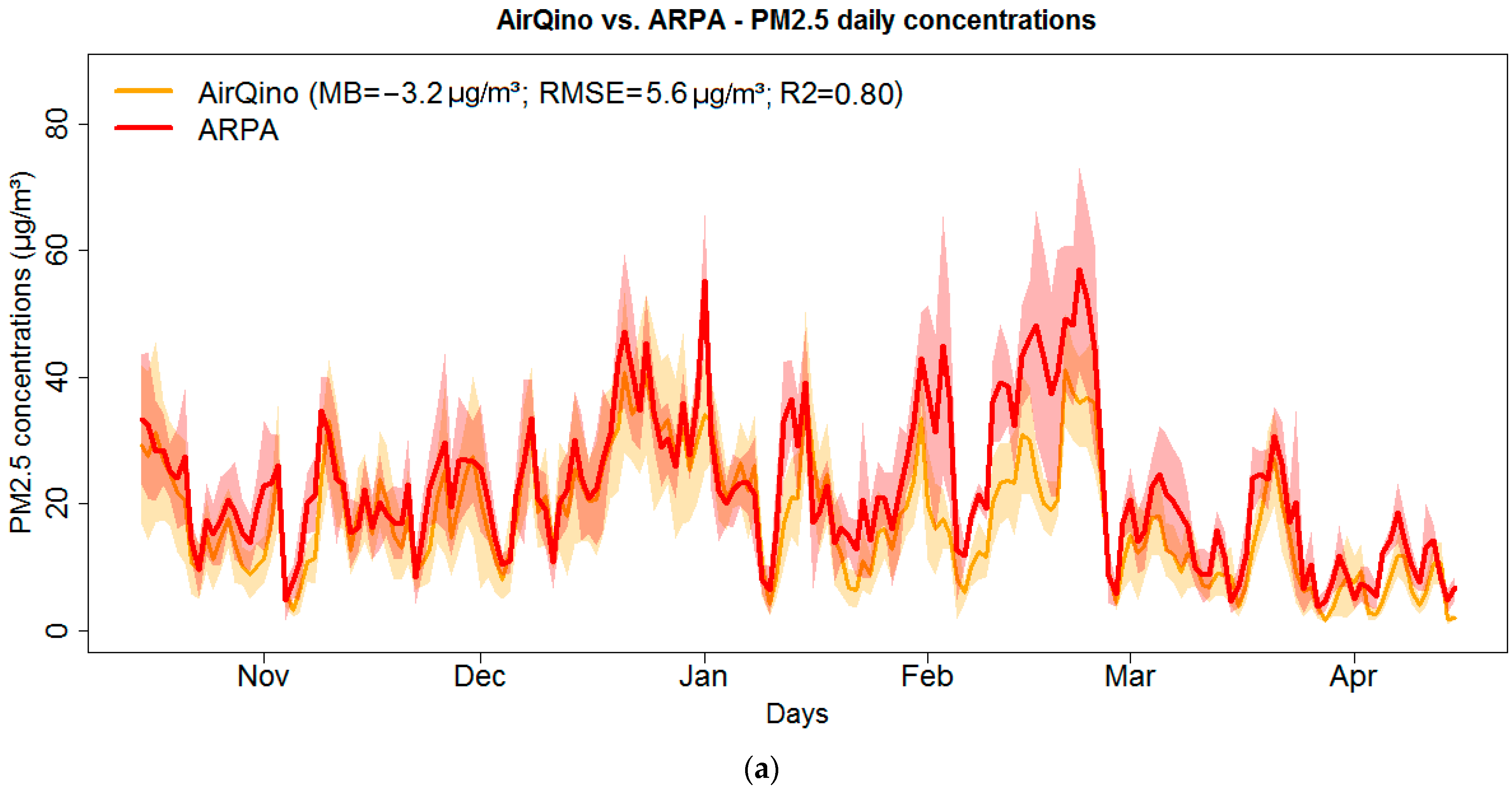
3.2. Scores by Station of Low-Cost Stations

The statistical scores exhibited by each LC station against the reference stations are detailed in Table 4 (PM2.5) and Table 5 (PM10 concentrations). The scores in monitoring the corresponding PM2.5/PM10 daily concentration ratios are reported in Table S5.
LC sensors were assessed in meeting the target values of US EPA “base” testing for PM2.5 air sensors (Table S3). Both the linear regression’s slope and intercept are concurrently met by four (out of nine) AirQino sensors, and by two (out of ten) PurpleAir sensors (Table 4). The linearity attribute (R2 ≥ 0.70) is satisfied by three AirQino and eight PurpleAir PM2.5 sensors. All LC sensors (except AirQino ID 184) lack precision, as the standard deviation of PM2.5 measured concentrations is above 5 μg/m3 (Table 2). Also, the attribute of error is systematically failed, as all LC sensors exhibit RMSE values above 7 μg/m3 (Table 4).
The boxplots of MB, MAE, RMSE and R2 distributions, exhibited by all LC stations as detailed in Table 4, Table 5 and Table S5, are plotted in Figure 4.
The analysis of MB boxplots (Figure 4a) reveals that AirQino stations tend to under-estimate both PM2.5 and PM10 concentrations observed by the reference stations, at worst under-estimating the former by 10.4 and the latter by 8.1 μg/m3 (Table 4). Conversely, PurpleAir stations both under- and over-estimate ARPA observations, also exhibiting a wider MB distribution—and thus higher MB extreme values—than AirQino stations (Figure 4a). AirQino MB scores are affected by a lower spread than PurpleAir, markedly in monitoring PM10 concentrations (σ = 3.5 vs. 11.7 μg/m3). In both MAE (Figure 4b) and RMSE (Figure 4c) boxplots and for both pollutants, AirQino stations exhibit better scores than PurpleAir stations, not only if considering the lower mean values (MAE = 8.4 ÷ 9.9 and RMSE = 10.8 ÷ 12.4 μg/m3), but also the narrower distributions’ full range. Conversely, PurpleAir outplays AirQino in R2 values related to both PM2.5 and PM10 daily concentrations (Figure 4d). If considering the full range of R2 distribution, in measuring PM2.5 concentrations, R2 spans 0.37 ÷ 0.78 for AirQino and 0.41 ÷ 0.86 for PurpleAir stations, while for PM10 concentrations, R2 spans 0.42 ÷ 0.76 (AirQino) and 0.37 ÷ 0.87 (PurpleAir, Table 4).
Both LC networks fail to reproduce magnitude (Figure 4a) and time variation (Figure 4d) of the PM2.5/PM10 ratio. In terms of MAE (Figure 4b) and RMSE (Figure 4c), PurpleAir stations are less inaccurate than AirQino stations.
The analysis of Taylor diagram provides further insight into LC station performances, markedly focusing on each individual station (Figure 5).
Several AirQino stations show a lower variability than ARPA reference stations (σLC < σARPA) in monitoring PM2.5 daily concentrations (Figure 5a), while PurpleAir stations exhibit a variability comparable or moderately higher than ARPA stations. PurpleAir stations show a lower centred RMSD and higher correlation coefficients than AirQino stations, with some points particularly close to the “ARPA observations” optimal point. In monitoring PM10 daily concentrations (Figure 5b), as shown by the cloud of points very close to each other, AirQino stations exhibit quite similar behaviour in all the three metrics of the Taylor diagram. Conversely, the PurpleAir station points show a large scatter, particularly in terms of variability with respect to ARPA variability. Also, in measuring PM10 daily concentrations, PurpleAir stations return a lower RMSD and higher correlation coefficients than AirQino stations.

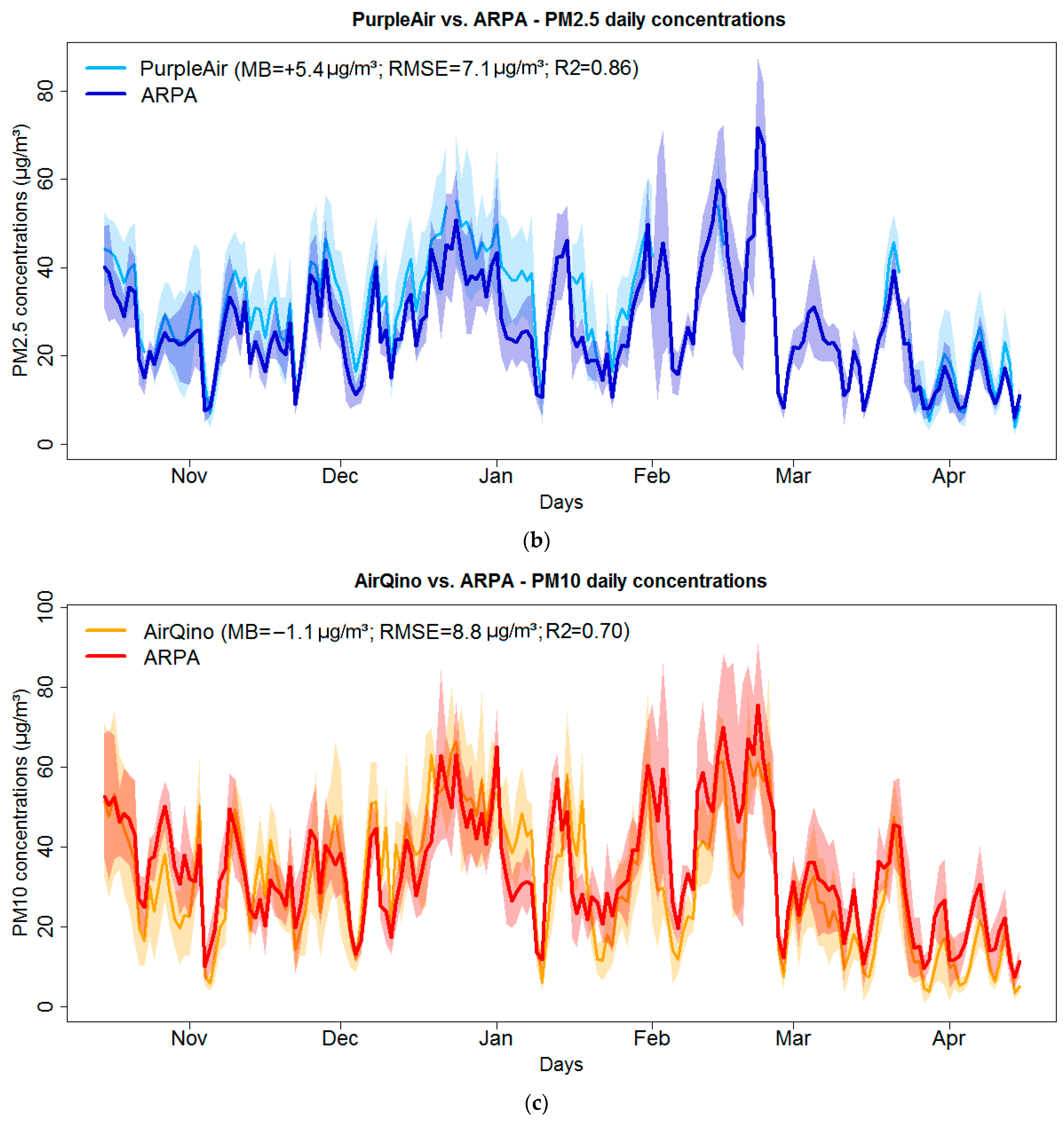
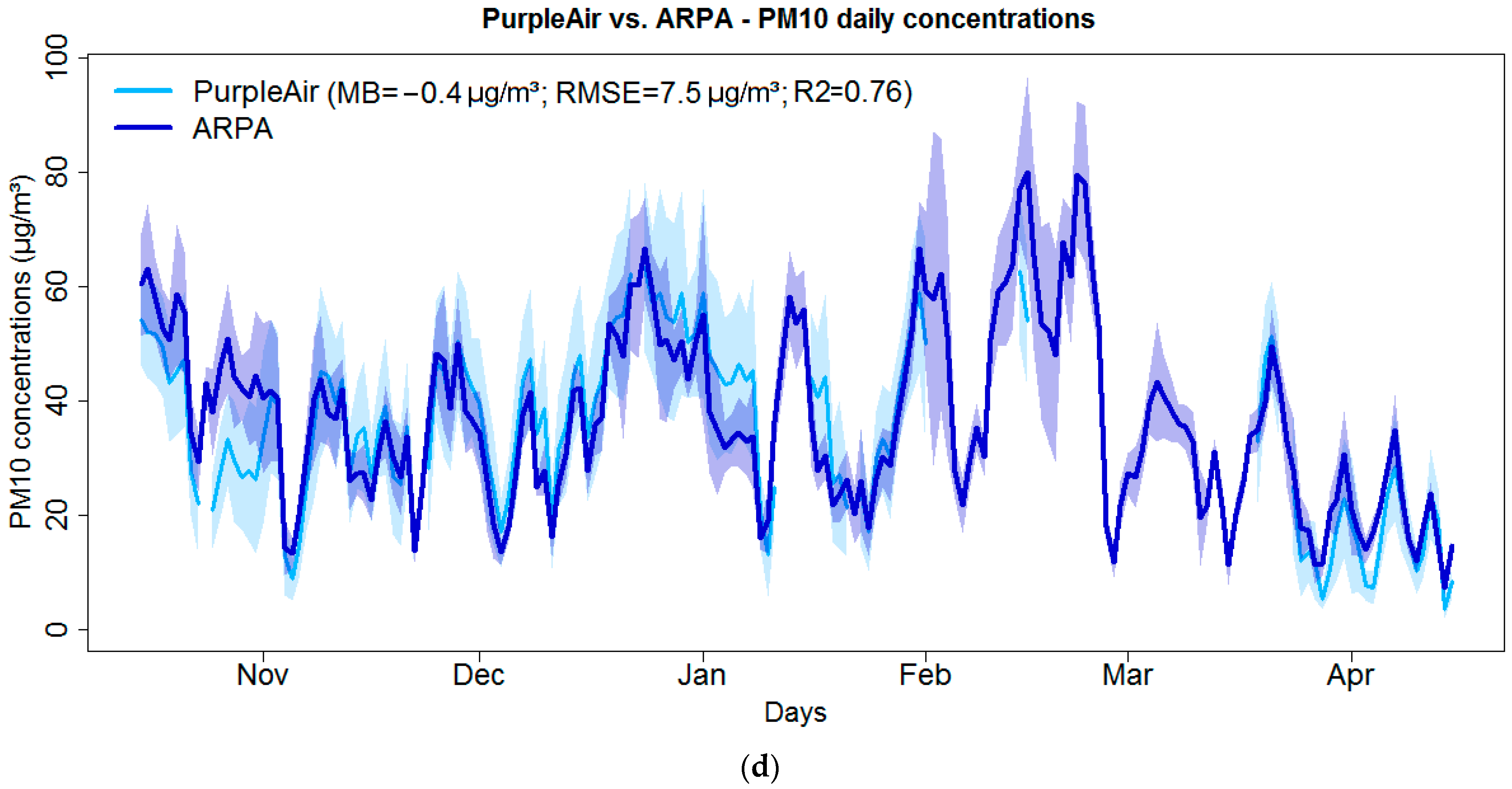
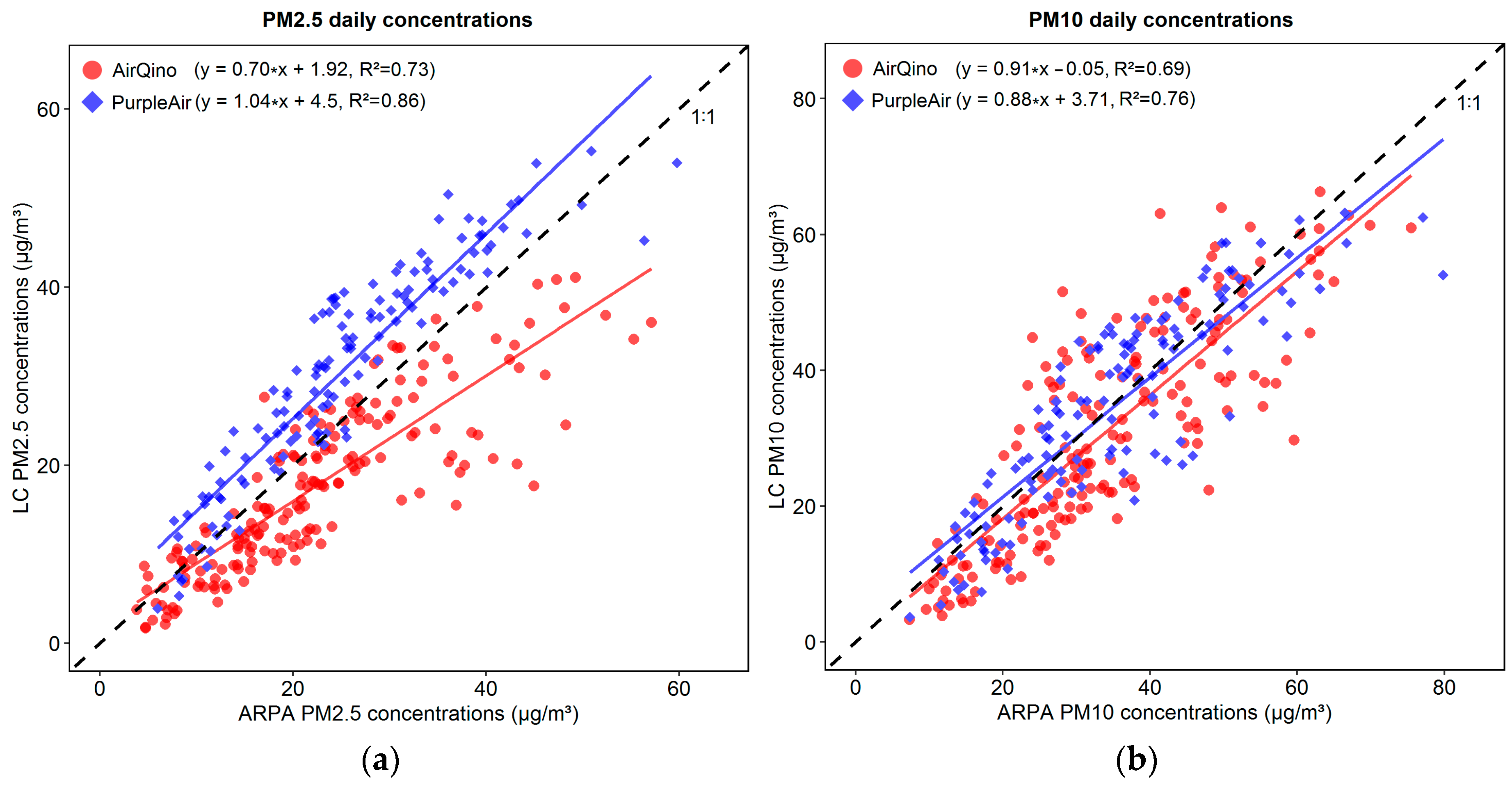
3.3. Overall Scores by Monitoring Network of Low-Cost Stations

Full time series of PM2.5 and PM10 daily concentrations averaged day-by-day by LC monitoring network vs. corresponding ARPA stations are plotted in Figure 6.
AirQino stations quite reasonably capture the pattern of ARPA PM2.5 concentrations, both in magnitude and time variation (RMSE = 5.6 μg/m3 and R2 = 0.80, Figure 6a). A closer analysis, however, reveals that AirQino measurements were particularly fine until late January and from March on, while they generally fail to reproduce ARPA observations during the month of February, i.e., when the highest ARPA concentrations are recorded. PurpleAir stations prove to remarkably capture the time variation of PM2.5 ARPA observations (R2 = 0.86, Figure 6b). Compared to AirQino stations, they exhibit better R2 values, while they exhibit worse values of MB (+5.4 μg/m3) and RMSE (7.1 μg/m3). However, it should be noted that PurpleAir PM2.5 observations were not available for comparison from early February to mid-March, which might possibly account for their overall better correlation than AirQino stations (R2 = 0.86 vs. 0.80). Compared to the case of PM2.5 concentrations, in monitoring PM10 concentrations, AirQino stations better fit the magnitude of reference observations, as returning an overall mean under-estimation of 1.1 μg/m3 (Figure 6c), while time variation is lower (R2 = 0.70). In this case, the February critical period appears to be better captured. Also, when monitoring PM10 concentrations (Figure 6d), PurpleAir stations better fit the magnitude (0.4 μg/m3 under-estimation) and time variation (R2 = 0.76) of reference observations with respect to AirQino stations, although, again, their missing values from early February to mid-March might affect this outcome.
Figure 7 shows the scatter plot between the PM2.5 and PM10 daily concentrations averaged day-by-day by LC monitoring network vs. corresponding ARPA stations.
Figure 7a confirms PurpleAir higher accuracy than AirQino in monitoring ARPA PM2.5 daily concentrations (R2 = 0.86 vs. 0.73). The slope of PurpleAir linear best fit basically matches that of the perfect agreement (1:1) line. Therefore, PurpleAir well reproduces ARPA PM2.5 daily observations over their full range, apart from a positive offset factor (4.5 μg/m3) indicating a systematic over-estimation. Conversely, AirQino tends to under-estimate PM2.5 reference observations, particularly at the highest values.
The pattern of the two LC networks is quite similar when focusing on PM10 concentrations, as highlighted by their almost matching best-fit lines (Figure 7b). Compared to ARPA observations, PurpleAir measurements slightly over-estimate at lower concentrations and slightly under-estimate at higher concentrations, while AirQino measurements slightly under-estimate almost across the full range of concentrations. Again, PurpleAir shows higher skills than AirQino in fitting the reference observations (R2 = 0.76 vs. 0.69).

4. Discussion

PM2.5 daily concentrations observed in the Padana Plain by the ARPA reference stations are in better agreement with the newly emerging AirQino sensors than the well-established PurpleAir sensors, with better values of MB, RMSE and MAE (Figure 4a–c). As for PM10 daily concentrations, PurpleAir sensors are more accurate in fitting the magnitude (Figure 4a), while less accurate in terms of RMSE and MAE (Figure 4b,c). This lower magnitude of the error exhibited by AirQino vs. PurpleAir stations might be due to the fact that their paired reference stations are located in environments affected by lower PM2.5 (Table 3) and PM10 concentrations (Table 4). By contrast, PurpleAir sensors are better at capturing the linearity of responses and time variation of both PM2.5 and PM10 daily concentrations, as shown with higher values of R2 (Figure 4d) and r (Figure 5). This confirms findings on sensor performance reported, e.g., by Badura et al. [48]. Furthermore, it might depend on the average distance of ARPA reference stations from PurpleAir stations, which is lower than that from AirQino stations for both PM2.5 (4.6 vs. 7.5 km, Table S1) and PM10 concentrations (4.8 vs. 9.0 km, Table S2). Current PurpleAir PM2.5 performance is consistent with that reported by Ardon-Dryer et al. [17] within a 2-year (January 2017 to December 2018) similar field assessment (no co-location) of 46 units vs. (gravimetric-based) regulatory stations in four US cities. As in Figure 4a, Figure 6b and Figure 7a, the majority of PurpleAir units measured PM2.5 concentrations higher than the reference stations. As suggested by Ardon-Dryer et al. [17], this could likely be due to changes in relative humidity, whose values are particularly high in winter in the Padana Plain.
Although a rigorous field validation (co-location vs. regulatory stations) was not performed in the present study, it is insightful to compare current LC sensor scores with those resulting from field validation studies addressed in the literature. Due to this reason, the present scores deserve more credit. Within a 4-month (September to December 2020) field validation of three PurpleAir units vs. a co-located (gravimetric-based) regulatory station in Vancouver (Canada), in monitoring PM2.5 daily concentrations Zimmerman [12] reported better scores (RMSE = 7.64–10.13 μg/m3, R2 = 0.91–0.94) than those achieved in the Padana Plain (RMSE = 7.9–19.7 μg/m3, R2 = 0.41–0.86, Table 4). PurpleAir tendency of over-estimating PM2.5 observed concentrations (Figure 4a and Figure 6b) is consistent with the findings by Zimmerman [12] and Barkjohn et al. [49], who reported that PurpleAir sensors over-estimated PM2.5 concentrations by about 40% in most parts of the US. Current PurpleAir R2 values in monitoring PM2.5 daily concentrations (Table 4 and Figure 4d) are worse than those (R2 > 0.88) achieved by Sayahi et al. [24] in Salt Lake City (USA), where they co-located for 320 days 2 PurpleAir units vs. a reference (gravimetric-based) station. Compared to the R2 values resulting from a 39-day (December 2016 to January 2017) field validation of three PurpleAir units vs. two (optical-based) regulatory stations in California (USA) [50], current results are worse for PM2.5 (R2 = 0.41–0.86 vs. 0.93–0.97, Table 4), while they are comparable for PM10 daily concentrations (R2 = 0.37–0.87 vs. 0.66–0.70, Table 5). Agreeing with findings in [50], in the Padana Plain, PurpleAir sensors are confirmed to be more accurate in monitoring PM2.5 than PM10 daily concentrations (Figure 4d). After deploying an AirQino unit close to an ARPA reference station in Florence (Italy) across a full “heating season” (November 2016 to April 2017), Cavaliere et al. [35] returned scores in measuring both PM2.5 (MB = +4.39 μg/m3, RMSE = 7.95 μg/m3 and R2 = 0.90) and PM10 daily concentrations (MB = +0.72 μg/m3, RMSE = 7.80 μg/m3 and R2 = 0.84) better than those achieved in the Padana Plain (Table 4 and Table 5). Within a 78-day co-location vs. an ARPA station in Capannori (Italy) across a spring period in 2019, Brilli et al. [36] reported AirQino scores in measuring PM2.5 daily concentrations to be both better (RMSE = 4.2 μg/m3 vs. 7.9–14.6 μg/m3) and worse (R2 = 0.54 vs. 0.37–0.78) than those achieved in the present study (Table 4). The AirQino scores reported in the same study in monitoring PM10 daily concentrations were better in terms of RMSE (4.6 μg/m3) and comparable in terms of R2 (0.63, Table 5).
The performance of the single sensors mounted on both PurpleAir and AirQino devices was also analyzed. Coker et al. [51] co-located for one year (January to December 2020) one Plantower MS5003 sensor to a reference (gravimetric-based) monitor installed at the US embassy in Kampala (Uganda). They reported scores in monitoring PM2.5 daily concentrations (RMSE = 14.43 μg/m3 and R2 = 0.76) quite in line with those achieved by the same sensors mounted on the PurpleAir units in the Padana Plain (Table 4). Three Novasense SDS011 sensors were tested by Božilov et al. [52] against a (gravimetric-based) reference monitor at two cities in Serbia for two 2-week heating periods between 2021 and 2022. In measuring PM2.5 concentrations, they found the RMSE to be ranging between 3.8 ÷ 22.4 μg/m3 and R2 0.55 ÷ 0.82, while in measuring PM10 concentrations, they reported the RMSE to be ranging between 11.1 ÷ 27.0 μg/m3 and R2 0.52 ÷ 0.80. Compared to those achieved in the Padana Plain by the same sensors mounted on the AirQino units, these scores are better in terms of R2 and worse in terms of RMSE (Table 4). Better R2 scores (0.87–0.90) in measuring PM2.5 daily concentrations were also achieved by Badura et al. [48] while testing three Novasense SDS011 sensors vs. a co-located (gravimetric-based) reference monitor in Wrocław (Poland) between August 2017 and February 2018.
The indicative compliance of current LC PM2.5 sensors to the US EPA “base” testing [39] was also explored. Assessed in meeting the corresponding target values (Table S3), the AirQino PM2.5 sensors show better bias and the PurpleAir PM2.5 sensors show better linearity (Table 4). Conversely, sensors belonging to both networks lack the attributes of precision (standard deviation above 5 μg/m3, Table 2) and error (RMSE above 7 μg/m3, Table 4).
If comparing LC sensor performance by pollutant, both PurpleAir and AirQino sensors exhibit higher accuracy in fitting the magnitude of PM10 than PM2.5 observations, while lower accuracy in terms of RMSE, MAE and R2 (Figure 4). This outcome is consistent with findings from the above studies for both PurpleAir [50] and AirQino sensors [35]. In monitoring PM2.5 concentrations, the PurpleAir sensors are stable across the full range of observations, unlike the AirQino sensors, whose under-estimations increase as the observations increase (Figure 7a). By contrast, in monitoring PM10 concentrations, the pattern of the two LC networks is similar (Figure 7b). This different behaviour per pollutant is noteworthy, particularly if considering that for both PurpleAir and AirQino sensors the PM2.5 and PM10 concentration outputs are produced after a mass conversion procedure based on a single input signal (Section 2.2.1 and Section 2.2.2). This is apparent in the PurpleAir sensors, whose PM2.5 outputs follow the 1:1 line (apart from an over-estimation offset factor, Figure 7a), while their PM10 outputs show a slight under-estimation trend (Figure 7b). Since Plantower PMS5003 sensors mounted on PurpleAir monitors are factory calibrated based on PM measurements collected in China [13], it can be recommended to introduce a correction factor to suitably reduce the estimated PM2.5/PM10 ratio. The latter (as shown in Figure 4a and in Table S5) is on average higher than the ARPA observed value. Likewise, since the Novasense SDS011 sensors mounted on AirQino monitors are factory calibrated based on China measurements as well, a correction should also be introduced to the AirQino outputs in order to increase (rather than decrease) their PM2.5/PM10 ratios. After these adjustments, the weight of fine fraction in total PM10 concentrations should be increased for AirQino and reduced for PurpleAir sensors. The boxplots of MAE (Figure 4b) and RMSE (Figure 4c) related to the PM2.5/PM10 ratios suggest that such corrections could be more successful for PurpleAir than AirQino sensors, since the former are affected by a lower discrepancy. In any case, the particularly low R2 values exhibited by both LC sensors (Figure 4d) suggest their inability at capturing the time variation of PM2.5/PM10 ratio.

5. Conclusions

In recent years, public availability of increasingly extensive LC sensor-based PM monitoring networks worldwide allowed researchers and citizen scientists to take huge advantage from the LC sensor technology. However, it should be borne in mind that most such sensors are only factory calibrated and factory calibration procedures are not specified in their datasheets [48]. Thus, a proper on-site calibration should necessarily be performed prior to using their data [52]. Unfortunately, this calibration is often not viable as LC sensors are frequently placed in regions where reference systems nearby are missing [17]. In the present study, the performance of two LC monitoring networks in measuring PM2.5 and PM10 concentrations compared to reference stations over a crucial PM hotspot such as the Padana Plain (Italy) was analyzed. Both the well-established PurpleAir and the newly emerging AirQino sensors returned good performance. AirQino sensors were finer in fitting the magnitude of PM2.5 concentrations, while PurpleAir sensors were in fitting that of PM10 concentrations. PurpleAir sensors were better at capturing the linearity and time variation of both PM2.5 and PM10 concentrations. Conversely, findings from several studies (e.g., [9,12,13,49]) were confirmed about LC sensor difficulties in correctly discriminating the size of individual particles as a result of the light-scattering PM sampling method they are based upon.
Indeed, finding a suitable tuning of the PM2.5 vs. PM10 outputs falls into an ever-wider research line aimed at developing the best correction techniques for LC sensors. Several such studies for PurpleAir sensors have been carried out in the literature. However, as pointed out by Barkjohn et al. [49], corrections have been developed for a specific region [22,28], season [24], or atmospheric condition [17], while few studies have addressed how widely applicable they are. Incorporating environmental factors such as air temperature and particularly relative humidity proved to return the finest scores [12,17,28,49]. However, finding the best correction algorithm valid for all application conditions remains a very challenging and certainly open issue that needs further efforts. This is particularly urgent in highly PM-polluted areas such as the Padana Plain. Here, high-granularity monitoring networks based on sufficiently reliable LC sensors could give a new dimension to air quality monitoring and democratize the whole process by making monitoring and results directly accessible at the community level [23].
The main limitation of this study lies in that, since the regulatory stations were not close enough to allow co-location, it was not possible to perform a rigorous field validation of the LC sensors. In addition, since regulatory observations were sampled at a daily resolution, PM2.5 and PM10 concentrations collected by the LC stations were assessed at 24 h rather than their native 1 h resolution. Future research lines could include deployment of new AirQino stations in the Padana Plain—hopefully very close to the existing ARPA stations—as well as using current PM observations from the two LC networks for validating PM forecasting products in the Padana Plain such as, e.g., the Copernicus Atmosphere Monitoring Service (CAMS).

Supplementary Materials

The following supporting information can be downloaded at: https://www.mdpi.com/article/10.3390/s24123946/s1, Figure S1: Sketch of the AirQino LC air quality monitoring unit; Table S1: Characteristics and pairing of ARPA reference stations used for validation of LC stations in measuring PM2.5 daily concentrations; Table S2: Characteristics and pairing of ARPA reference stations used for validation of LC stations in measuring PM10 daily concentrations; Table S3: Performance metrics and target values recommended by US EPA for PM2.5 air sensors used for non-regulatory supplemental and informational monitoring applications in ambient, outdoor and fixed-site environments: “base” testing [39]; Table S4: Statistics of PM2.5/PM10 daily concentration ratio measured by LC stations and corresponding paired ARPA reference stations (15 October 2022–15 April 2023); Table S5: Statistical scores of LC stations compared to ARPA reference stations in measuring the PM2.5/PM10 daily concentration ratio (15 October 2022–15 April 2023).

Author Contributions

Conceptualization, G.G. and B.G.; methodology, G.G.; software, G.G.; investigation, G.G. and B.G.; validation, G.G.; formal analysis, G.G. and T.G.; data curation, G.G., A.C. and T.G.; visualization, G.G.; writing—original draft preparation, G.G. and C.V.; writing—review and editing, L.B., F.C., A.C., T.G., S.P., A.Z. and B.G.; supervision, B.G. All authors have read and agreed to the published version of the manuscript.

Funding

This research received no external funding.

Institutional Review Board Statement

Not applicable.

Informed Consent Statement

Not applicable.

Data Availability Statement

Acknowledgments

The authors wish to thank ARPA Veneto for kindly providing the PM2.5 and PM10 concentration observations collected by the air quality monitoring stations in the Veneto region.

Conflicts of Interest

The authors declare no conflicts of interest.

References

  1. WHO. Ambient (Outdoor) Air Pollution. Available online: https://www.who.int/data/gho/data/themes/air-pollution (accessed on 16 April 2024).
  2. EEAa. Europe’s Air Quality Status 2023. Available online: https://www.eea.europa.eu/publications/europes-air-quality-status-2023. (accessed on 16 April 2024).
  3. Bigi, A.; Ghermandi, G. Trends and variability of atmospheric PM2.5 and PM10–2.5 concentration in the Po Valley, Italy. Atmos. Chem. Phys. 2016, 16, 15777–15788. [Google Scholar] [CrossRef]
  4. EEAb. Air Quality Statistics. Available online: https://www.eea.europa.eu/data-and-maps/dashboards/air-quality-statistics (accessed on 16 April 2024).
  5. Gualtieri, G.; Brilli, L.; Carotenuto, F.; Vagnoli, C.; Zaldei, A.; Gioli, B. Long-Term COVID-19 Restrictions in Italy to Assess the Role of Seasonal Meteorological Conditions and Pollutant Emissions on Urban Air Quality. Atmosphere 2022, 13, 1156. [Google Scholar] [CrossRef]
  6. Bart, M.; E Williams, D.; Ainslie, B.; McKendry, I.; Salmond, J.; Grange, S.K.; Alavi-Shoshtari, M.; Steyn, D.; Henshaw, G.S. High density ozone monitoring using gas sensitive semi-conductor sensors in the Lower Fraser Valley, British Columbia. Environ. Sci. Technol. 2014, 48, 3970–3977. [Google Scholar] [CrossRef] [PubMed]
  7. Carotenuto, F.; Bisignano, A.; Brilli, L.; Gualtieri, G.; Giovannini, L. Low-cost air quality monitoring networks for long-term field campaigns: A review. Meteorol. Appl. 2023, 30, e2161. [Google Scholar] [CrossRef]
  8. Castell, N.; Dauge, F.R.; Schneider, P.; Vogt, M.; Lerner, U.; Fishbain, B.; Broday, D.; Bartonova, A. Can commercial low-cost sensor platforms contribute to air quality monitoring and exposure estimates? Environ. Int. 2017, 99, 293–302. [Google Scholar] [CrossRef] [PubMed]
  9. Morawska, L.; Thai, P.K.; Liu, X.; Asumadu-Sakyi, A.; Ayoko, G.; Bartonova, A.; Bedini, A.; Chai, F.; Christensen, B.; Dunbabin, M.; et al. Applications of low-cost sensing technologies for air quality monitoring and exposure assessment: How far have they gone? Environ. Int. 2018, 116, 286–299. [Google Scholar] [CrossRef] [PubMed]
  10. Tryner, J.; L’Orange, C.; Mehaffy, J.; Miller-Lionberg, D.; Hofstetter, J.C.; Wilson, A.; Volckens, J. Laboratory evaluation of low-cost PurpleAir PM monitors and in-field correction using co-located portable filter samplers. Atmos. Environ. 2020, 220, 117067. [Google Scholar] [CrossRef]
  11. Karagulian, F.; Barbiere, M.; Kotsev, A.; Spinelle, L.; Gerboles, M.; Lagler, F.; Redon, N.; Crunaire, S.; Borowiak, A. Review of the performance of low-cost sensors for air quality monitoring. Atmosphere 2019, 10, 506. [Google Scholar] [CrossRef]
  12. Zimmerman, N. Tutorial: Guidelines for implementing low-cost sensor networks for aerosol monitoring. J. Aerosol Sci. 2022, 159, 105872. [Google Scholar] [CrossRef]
  13. Malings, C.; Tanzer, R.; Hauryliuk, A.; Saha, P.K.; Robinson, A.L.; Presto, A.A.; Subramanian, R. Fine particle mass monitoring with low-cost sensors: Corrections and long-term performance evaluation. Aerosol Sci. Technol. 2020, 54, 160–174. [Google Scholar] [CrossRef]
  14. Bi, J.; Carmona, N.; Blanco, M.N.; Gassett, A.J.; Seto, E.; Szpiro, A.A.; Larson, T.V.; Sampson, P.D.; Kaufman, J.D.; Sheppard, L. Publicly available low-cost sensor measurements for PM2.5 exposure modeling: Guidance for monitor deployment and data selection. Environ. Int. 2022, 158, 106897. [Google Scholar] [CrossRef] [PubMed]
  15. Raysoni, A.U.; Pinakana, S.D.; Mendez, E.; Wladyka, D.; Sepielak, K.; Temby, O. A Review of Literature on the Usage of Low-Cost Sensors to Measure Particulate Matter. Earth 2023, 4, 168–186. [Google Scholar] [CrossRef]
  16. AQ-SPECa. PM Sensor Evaluations. Available online: http://www.aqmd.gov/aq-spec/evaluations/summary-pm (accessed on 16 April 2024).
  17. Ardon-Dryer, K.; Dryer, Y.; Williams, J.N.; Moghimi, N. Measurements of PM2.5 with PurpleAir under atmospheric conditions. Atmos. Meas. Tech. 2020, 13, 5441–5458. [Google Scholar] [CrossRef]
  18. ISTAT. Gross Domestic Product Supply Side. Available online: http://dati.istat.it/Index.aspx?QueryId=11455&lang=en (accessed on 16 April 2024).
  19. ISTAT. Classification of Municipalities Based on Italian Ecoregions. 12 October 2023. Available online: https://www.istat.it/en/archivio/224797 (accessed on 16 April 2024).
  20. Gualtieri, G.; Carotenuto, F.; Finardi, S.; Tartaglia, M.; Toscano, P.; Gioli, B. Forecasting PM10 hourly concentrations in northern Italy: Insights on models performance and PM10 drivers through self-organizing maps. Atmos. Pollut. Res. 2018, 9, 1204–1213. [Google Scholar] [CrossRef]
  21. Bigi, A.; Ghermandi, G.; Harrison, R.M. Analysis of the air pollution climate at a background site in the Po valley. J. Environ. Monitor. 2012, 14, 552–563. [Google Scholar] [CrossRef] [PubMed]
  22. Bi, J.; Wildani, A.; Chang, H.H.; Liu, Y. Incorporating low-cost sensor measurements into high-resolution PM2.5 modeling at a large spatial scale. Environ. Sci. Technol. 2020, 54, 2152–2162. [Google Scholar] [CrossRef] [PubMed]
  23. Farooqui, Z.; Biswas, J.; Saha, J. Long-Term Assessment of PurpleAir Low-Cost Sensor for PM2.5 in California, USA. Pollutants 2023, 3, 477–493. [Google Scholar] [CrossRef]
  24. Sayahi, T.; Butterfield, A.; Kelly, K.E. Long-term field evaluation of the Plantower PMS low-cost particulate matter sensors. Environ. Pollut. 2019, 245, 932–940. [Google Scholar] [CrossRef] [PubMed]
  25. Tanzer, R.; Malings, C.; Hauryliuk, A.; Subramanian, R.; Presto, A.A. Demonstration of a low-cost multi-pollutant network to quantify intra-urban spatial variations in air pollutant source impacts and to evaluate environmental justice. Int. J. Environ. Res. Public Health 2019, 16, 2523. [Google Scholar] [CrossRef]
  26. Delp, W.W.; Singer, B.C. Wildfire smoke adjustment factors for low-cost and professional PM2.5 monitors with optical sensors. Sensors 2020, 20, 3683. [Google Scholar] [CrossRef]
  27. Mei, H.; Han, P.; Wang, Y.; Zeng, N.; Liu, D.; Cai, Q.; Deng, Z.; Wang, Y.; Pan, Y.; Tang, X. Field evaluation of low-cost particulate matter sensors in Beijing. Sensors 2020, 20, 4381. [Google Scholar] [CrossRef] [PubMed]
  28. Stavroulas, I.; Grivas, G.; Michalopoulos, P.; Liakakou, E.; Bougiatioti, A.; Kalkavouras, P.; Fameli, K.M.; Hatzianastassiou, N.; Mihalopoulos, N.; Gerasopoulos, E. Field Evaluation of Low-Cost PM Sensors (Purple Air PA-II) Under Variable Urban Air Quality Conditions, in Greece. Atmosphere 2020, 11, 926. [Google Scholar] [CrossRef]
  29. Awokola, B.I.; Okello, G.; Mortimer, K.J.; Jewell, C.P.; Erhart, A.; Semple, S. Measuring air quality for advocacy in Africa (MA3): Feasibility and practicality of longitudinal ambient PM2.5 measurement using low-cost sensors. Int. J. Environ. Res. Public Health 2020, 17, 7243. [Google Scholar] [CrossRef] [PubMed]
  30. Hasenkopf, C.A. Sharing lessons-learned on effective open data, open-source practices from OpenAQ, a global open air quality community. AGU Fall Meet. Abstr. 2017, 2017, IN44A-08. [Google Scholar]
  31. Gualtieri, G.; Camilli, F.; Cavaliere, A.; De Filippis, T.; Di Gennaro, F.; Di Lonardo, S.; Dini, F.; Gioli, B.; Matese, A.; Nunziati, W.; et al. An integrated low-cost road traffic and air pollution monitoring platform to assess vehicles’ air quality impact in urban areas. Transp. Res. Procedia 2017, 27, 609–616. [Google Scholar] [CrossRef]
  32. Vagnoli, C.; Martelli, F.; De Filippis, T.; Di Lonardo, S.; Gioli, B.; Gualtieri, G.; Matese, A.; Rocchi, L.; Toscano, P.; Zaldei, A. The SensorWebBike for air quality monitoring in a smart city. In Proceedings of the IET Conference on Future Intelligent Cities, London, UK, 4–5 December 2014. [Google Scholar] [CrossRef]
  33. Zaldei, A.; Vagnoli, C.; Di Lonardo, S.; Gioli, B.; Gualtieri, G.; Toscano, P.; Martelli, F.; Matese, A. AIRQino, a low-cost air quality mobile platform. In Proceedings of the EGU General Assembly Conference Abstracts, Vienna, Austria, 12–17 April 2015. [Google Scholar]
  34. Gualtieri, G.; Ahbil, K.; Brilli, L.; Carotenuto, F.; Cavaliere, A.; Gioli, B.; Giordano, T.; Katiellou, G.L.; Mouhaimini, M.; Tarchiani, V.; et al. Potential of low-cost PM monitoring sensors to fill monitoring gaps in areas of Sub-Saharan Africa. Atmos. Pollut. Res. 2024, 15, 102158. [Google Scholar] [CrossRef]
  35. Cavaliere, A.; Carotenuto, F.; Di Gennaro, F.; Gioli, B.; Gualtieri, G.; Martelli, F.; Matese, A.; Toscano, P.; Vagnoli, C.; Zaldei, A. Development of low-cost air quality stations for next generation monitoring networks: Calibration and validation of PM2.5 and PM10 sensors. Sensors 2018, 18, 2843. [Google Scholar] [CrossRef] [PubMed]
  36. Brilli, L.; Carotenuto, F.; Andreini, B.P.; Cavaliere, A.; Esposito, A.; Gioli, B.; Martelli, F.; Stefanelli, M.; Vagnoli, C.; Venturi, S.; et al. Low-Cost Air Quality Stations’ Capability to Integrate Reference Stations in Particulate Matter Dynamics Assessment. Atmosphere 2021, 12, 1065. [Google Scholar] [CrossRef]
  37. Carotenuto, F.; Brilli, L.; Gioli, B.; Gualtieri, G.; Vagnoli, C.; Mazzola, M.; Viola, A.P.; Vitale, V.; Severi, M.; Traversi, R.; et al. Long-term performance assessment of low-cost atmospheric sensors in the arctic environment. Sensors 2020, 20, 1919. [Google Scholar] [CrossRef]
  38. Zikova, N.; Masiol, M.; Chalupa, D.C.; Rich, D.Q.; Ferro, A.R.; Hopke, P.K. Estimating hourly concentrations of PM2.5 across a metropolitan area using low-cost particle monitors. Sensors 2017, 17, 1922. [Google Scholar] [CrossRef]
  39. Duvall, R.; Clements, A.; Hagler, G.; Kamal, A.; Kilaru, V.; Goodman, L.; Frederick, S.; Barkjohn, K.; VonWald, I.; Greene, D.; et al. Performance Testing Protocols, Metrics, and Target Values for Fine Particulate Matter Air Sensors: Use in Ambient, Outdoor, Fixed Site, Non-Regulatory Supplemental and Informational Monitoring Applications; EPA/600/R-20/280, Technical Report; U.S. EPA Office of Research and Development: Washington, DC, USA, 2021. Available online: https://cfpub.epa.gov/si/si_public_record_Report.cfm?dirEntryId=350785&Lab=CEMM (accessed on 16 April 2024).
  40. R Core Team. The R Project for Statistical Computing. Available online: https://www.r-project.org (accessed on 16 April 2024).
  41. R Package “pastecs”: Package for Analysis of Space-Time Ecological Series (Version 1.4.2). Available online: https://cran.r-project.org/web/packages/pastecs/index.html (accessed on 16 April 2024).
  42. R Package “Metrics”: Evaluation Metrics for Machine Learning (Version 0.1.4). Available online: https://cran.r-project.org/web/packages/Metrics/index.html (accessed on 16 April 2024).
  43. R Stats Package. Version 4.5.0. Available online: https://stat.ethz.ch/R-manual/R-devel/library/stats/html/00Index.html (accessed on 16 April 2024).
  44. R Graphics Package. Version 4.5.0. Available online: https://stat.ethz.ch/R-manual/R-devel/library/graphics/html/00Index.html (accessed on 16 April 2024).
  45. R package “ggplot2”: Create Elegant Data Visualisations Using the Grammar of Graphics (Version 3.5.0). Available online: https://cran.r-project.org/web/packages/ggplot2/index.html (accessed on 16 April 2024).
  46. Carslaw, D.C.; Ropkins, K. Openair—An R package for air quality data analysis. Environ. Model. Softw. 2012, 27–28, 52–61. [Google Scholar] [CrossRef]
  47. Taylor, K.E. Summarizing multiple aspects of model performance in a single diagram. J. Geoph. Res. 2001, 106, 7183–7192. [Google Scholar] [CrossRef]
  48. Badura, M.; Batog, P.; Drzeniecka-Osiadacz, A.; Modzel, P. Evaluation of low-cost sensors for ambient PM2.5 monitoring. J. Sens. 2018, 2018, 5096540. [Google Scholar] [CrossRef]
  49. Barkjohn, K.K.; Gantt, B.; Clements, A.L. Development and application of a United States-wide correction for PM2.5 data collected with the PurpleAir sensor. Atmos. Meas. Tech. 2021, 14, 4617–4637. [Google Scholar] [CrossRef] [PubMed]
  50. AQ-SPECb. Evaluation Summary of PurpleAir PA-II. Available online: http://www.aqmd.gov/docs/default-source/aq-spec/summary/purpleair-pa-ii---summary-report.pdf?sfvrsn=16 (accessed on 16 April 2024).
  51. Coker, E.S.; Amegah, A.K.; Mwebaze, E.; Ssematimba, J.; Bainomugisha, E. A land use regression model using machine learning and locally developed low cost particulate matter sensors in Uganda. Environ. Res. 2021, 199, 111352. [Google Scholar] [CrossRef]
  52. Božilov, A.; Tasić, V.; Živković, N.; Lazović, I.; Blagojević, M.; Mišić, N.; Topalović, D. Performance assessment of NOVA SDS011 low-cost PM sensor in various microenvironments. Environ. Monit. Assess. 2022, 194, 595. [Google Scholar] [CrossRef]
Figure 1. Map of the Padana Plain (green shaded area) in Italy, also showing the full operating LC PM2.5 and PM10 monitoring networks: AirQino (red dots); PurpleAir (cyan diamonds). Cartography basemap: Bing.
Sensors 24 03946 g001
Figure 2. Map of PM2.5 and PM10 monitoring stations analyzed in the study: AirQino LC sensors (red dots); PurpleAir LC sensors (cyan diamonds); ARPA reference stations (yellow squares). Cartography basemap: Bing.
Sensors 24 03946 g002
Figure 3. Map of full period averaged daily concentrations of (a) PM2.5 and (b) PM10 measured by LC stations and corresponding paired ARPA reference stations (15 October 2022–15 April 2023).
Sensors 24 03946 g003
Figure 4. Boxplots of statistical skill scores of LC stations vs. ARPA reference stations in monitoring daily concentrations of PM2.5, PM10 and PM2.5/PM10 ratio (15 October 2022–15 April 2023): (a) mean bias; (b) mean absolute error; (c) root mean square error; (d) coefficient of determination. Boxplots are delimited by the first (Q1) and third (Q3) distribution’s quartiles, while the black line inside the box denotes the median value (Q2). The mean and standard deviation values by pollutant for each LC network are reported in brackets.
Sensors 24 03946 g004
Figure 5. Taylor diagrams of (a) PM2.5 and (b) PM10 daily concentrations observed by all single LC stations compared to the paired ARPA reference stations (15 October 2022–15 April 2023). Dashed black circles (radial distance from the origin) show standard deviation of LC observations (σLC) normalized to standard deviation of ARPA observations (σARPA). Concentric dashed yellow circles emanating from ARPA observations point show a centred root mean square difference (RMSD), which is also normalized to σARPA. RMSD is centred as mean values of LC and ARPA observations are subtracted first: therefore, the diagram does not provide information about overall biases [47].
Sensors 24 03946 g005
Figure 6. Time series of daily concentrations averaged by LC monitoring network compared to corresponding ARPA reference stations (15 October 2022–15 April 2023): (a) AirQino PM2.5; (b) PurpleAir PM2.5; (c) AirQino PM10; (d) PurpleAir PM10. For each LC monitoring network, mean bias, root mean square error and coefficient of determination are also shown. The shaded areas show the confidence interval at 95% level around the mean values.
Sensors 24 03946 g006aSensors 24 03946 g006bSensors 24 03946 g006c
Figure 7. Scatter plots between daily concentrations averaged by LC monitoring network and corresponding ARPA reference stations (15 October 2022–15 April 2023): (a) PM2.5; (b) PM10. The best linear fit for each LC network, along with the corresponding equation (y = a * x + b, in brackets), are also shown as compared to the 1:1 black dashed line.
Sensors 24 03946 g007
Table 1. Characteristics of LC air quality stations sorted by monitoring network and ARPA reference stations available for assessment 1.
NetworkIDType 2Latitude (Deg N)Longitude (Deg E)Elevation (m a.s.l.)Assessment vs. ARPA Stations 3
PM2.5PM10
AirQino34RB44.533611.273638xx
42SB45.422010.934375xx
96RB44.392911.795919xx
132SB45.55629.1422158xx
135RT45.55759.1520159xx
158RT45.412911.131542xx
171UB45.01947.6285246xx
172RB44.96517.5732245xx
184SB45.952312.691423x
PurpleAir64303UB45.527110.2230131xx
65684SB45.00399.619686xx
66626RB45.59028.1347383xx
71131UT44.635110.920836xx
73781SB45.548212.079714 x
218818SB45.32528.8417112 x
229086UB45.409511.889512xx
230713UT45.18279.146065xx
230729RB45.18039.191373xx
230732RB45.19949.181481xx
292327SB45.03757.7728455xx
299967SB45.294511.81667xx
1 Geographic location of LC air quality stations is presented in Figure 2. 2 Station type: UB Urban background; RB, Rural background; SB, Suburban background; UT, Urban traffic; RT, Rural traffic. 3 Assessment of PM2.5 and PM10 LC sensors is subject to availability of complying ARPA stations.
Table 2. Statistics of PM2.5 daily concentrations measured by LC stations and corresponding paired ARPA reference stations (15 October 2022–15 April 2023).
LC StationsARPA Stations
NetworkIDType 1Valid Data (%) 2PM2.5 Concentrations (µg/m3)PM2.5 Concentrations (µg/m3)
MeanSt.dev. 4MeanSt.dev.
AirQino34RB92.420.214.117.610.7
42SB75.421.213.720.815.0
96RB60.79.15.515.29.9
132SB91.818.711.326.813.0
135RT92.925.616.322.811.1
158RT78.716.311.525.118.5
171UB91.320.19.025.512.1
172RB89.615.07.225.211.5
184SB65.66.03.216.49.0
Overall 3 17.89.522.511.5
PurpleAir64303UB65.035.316.328.412.8
65684SB66.740.018.925.512.2
66626RB65.027.814.113.87.0
71131UT69.439.315.023.711.6
229086UB66.733.716.429.217.2
230713UT58.516.011.227.011.9
230729RB61.234.514.926.212.3
230732RB58.517.58.626.112.2
292327SB66.127.612.026.613.0
299967SB65.037.618.329.016.2
Overall 3 30.512.126.412.1
1 Station type: UB, urban background; RB, rural background; SB, suburban background; UT, urban traffic; RT, rural traffic. 2 For each LC station and pollutant, valid data refer to the sample of concurrently available LC and ARPA observations. 3 Overall values by monitoring network of mean concentrations averaged across the full period are based on day-by-day values averaged across all LC or ARPA stations. 4 Values in bold for standard deviation denote LC stations meeting US EPA target values recommended for PM2.5 air sensors (Table S3).
Table 3. Statistics of PM10 daily concentrations measured by LC stations and corresponding paired ARPA reference stations (15 October 2022–15 April 2023).
LC StationsARPA Stations
NetworkIDType 1Valid Data (%) 2PM10 Concentrations (µg/m3)PM10 Concentrations (µg/m3)
MeanSt.dev.MeanSt.dev.
AirQino34RB96.723.216.426.913.5
42SB79.231.018.134.517.8
96RB63.417.59.524.312.0
132SB85.831.319.532.817.0
135RT97.338.223.138.817.3
158RT92.428.119.536.217.0
171UB90.736.819.833.716.1
172RB92.431.516.233.314.7
Overall 3 31.215.934.314.5
PurpleAir64303UB66.141.919.839.515.7
65684SB67.851.026.333.915.7
66626RB68.932.717.525.310.5
71131UT70.547.719.741.218.9
73781SB71.033.819.038.025.2
218818SB62.312.47.033.017.6
229086UB68.941.422.136.520.1
230713UT66.717.613.735.817.0
230729RB67.841.318.633.815.4
230732RB65.020.310.533.715.2
292327SB65.632.715.635.816.4
299967SB68.344.422.935.919.1
Overall 3 34.514.836.815.8
1 Station type: UB, urban background; RB, rural background; SB, suburban background; UT, urban traffic; RT, rural traffic. 2 For each LC station and pollutant, valid data refer to the sample of concurrently available LC and ARPA observations. 3 Overall values by monitoring network of mean concentrations averaged across the full period are based on day-by-day values averaged across all LC or ARPA stations.
Table 4. Statistical scores of LC stations compared to ARPA reference stations in measuring PM2.5 daily concentrations (15 October 2022–15 April 2023) 1,2.
NetworkIDValid Data (%)MB (µg/m3)MAE (µg/m3)SlopeIntercept (µg/m3)RMSE (µg/m3)R2
AirQino3492.4+2.66.61.061.58.70.65
4275.4+0.48.50.647.911.20.49
9660.7−6.27.10.334.010.00.37
13291.8−8.18.60.73−0.810.80.70
13592.9+2.87.01.25−2.99.40.72
15878.7−8.811.00.503.814.60.64
17191.3−5.46.30.663.47.90.78
17289.6−10.110.30.492.712.50.61
18465.6−10.410.50.251.812.60.51
PurpleAir6430365.0+7.08.41.152.810.10.81
6568466.7+14.615.31.1111.819.70.51
6662665.0+14.014.21.852.316.20.85
7113169.4+15.615.71.1212.817.40.74
22908666.7+4.56.20.888.07.90.86
23071358.5−11.011.10.81−5.912.70.74
23072961.2+8.49.21.115.510.40.83
23073258.5−8.68.60.650.610.20.85
29232766.1+1.07.90.6011.710.60.41
29996765.0+8.69.11.047.311.00.86
1 All R2 scores significant at 1% level (p < 0.05). 2 Values in bold for slope, intercept, RMSE and R2 denote LC stations meeting US EPA target values recommended for PM2.5 air sensors (Table S3).
Table 5. Statistical scores of LC stations compared to ARPA reference stations in measuring PM10 daily concentrations (15 October 2022–15 April 2023) 1.
NetworkIDValid Data (%)MB (µg/m3)MAE (µg/m3)SlopeIntercept (µg/m3)RMSE (µg/m3)R2
AirQino3496.7−3.89.20.92−1.711.30.58
4279.2−3.410.30.784.312.80.58
9663.4−6.88.80.525.011.40.42
13285.8−1.510.80.843.713.50.54
13597.3−0.610.91.06−3.014.00.63
15892.4−8.112.50.89−4.114.80.61
17190.7+3.27.71.070.810.30.76
17292.4−1.98.70.833.811.10.57
PurpleAir6430366.1+2.49.11.07−0.510.70.73
6568467.8+17.120.41.0216.426.90.37
6662668.9+7.49.71.47−4.412.20.77
7113170.5+6.611.70.8413.113.70.65
7378171.0−4.28.10.697.611.80.83
21881862.3−20.620.60.350.823.70.79
22908668.9+5.07.61.034.09.40.87
23071366.7−18.118.20.58−3.121.70.51
23072967.8+7.511.01.007.312.70.69
23073265.0−13.413.40.571.216.10.67
29232765.6−3.110.00.6011.214.00.40
29996768.3+8.510.01.114.612.30.86
1 All R2 scores significant at 1% level (p < 0.05).
Disclaimer/Publisher’s Note: The statements, opinions and data contained in all publications are solely those of the individual author(s) and contributor(s) and not of MDPI and/or the editor(s). MDPI and/or the editor(s) disclaim responsibility for any injury to people or property resulting from any ideas, methods, instructions or products referred to in the content.

