

Photovoltaic Power Injection Control Based on a Virtual Synchronous Machine Strategy


 ,
,  , and
, and 
Abstract
:1. Introduction
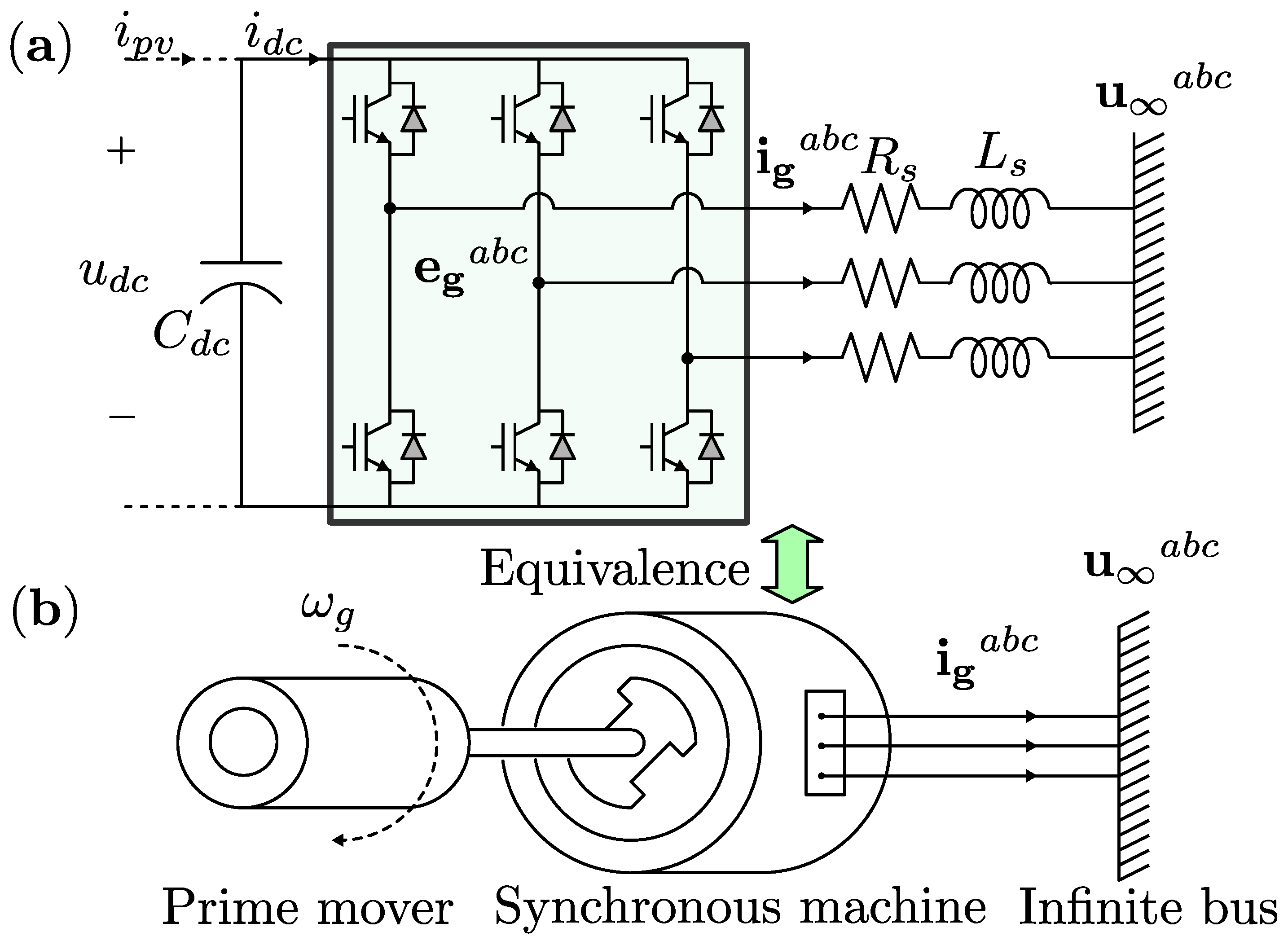
2. System Equations
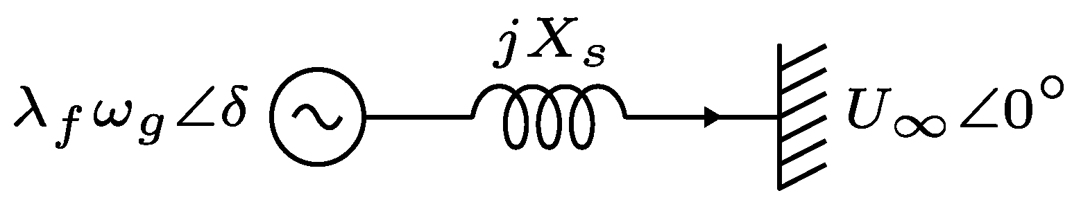
2.1. Power System Equations
2.2. Synchronverter Equations
2.3. DC Voltage Control Loop
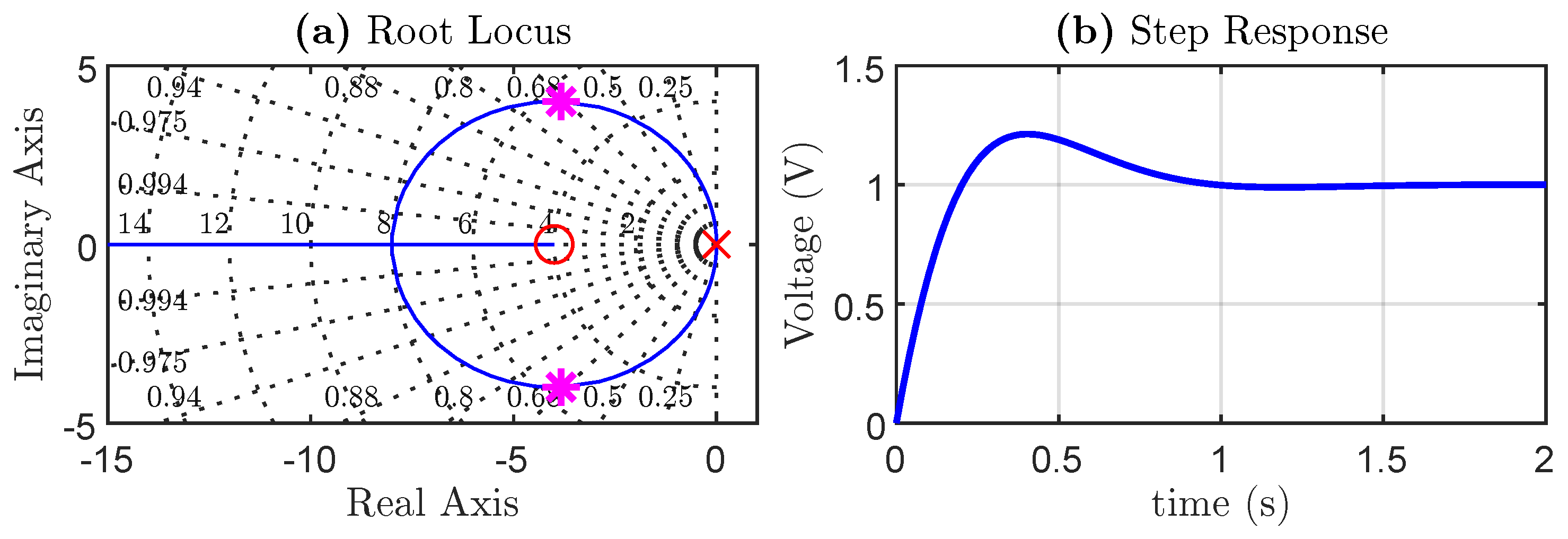
3. Small-Signal Analysis of the Synchronverter
3.1. Active Power Loop
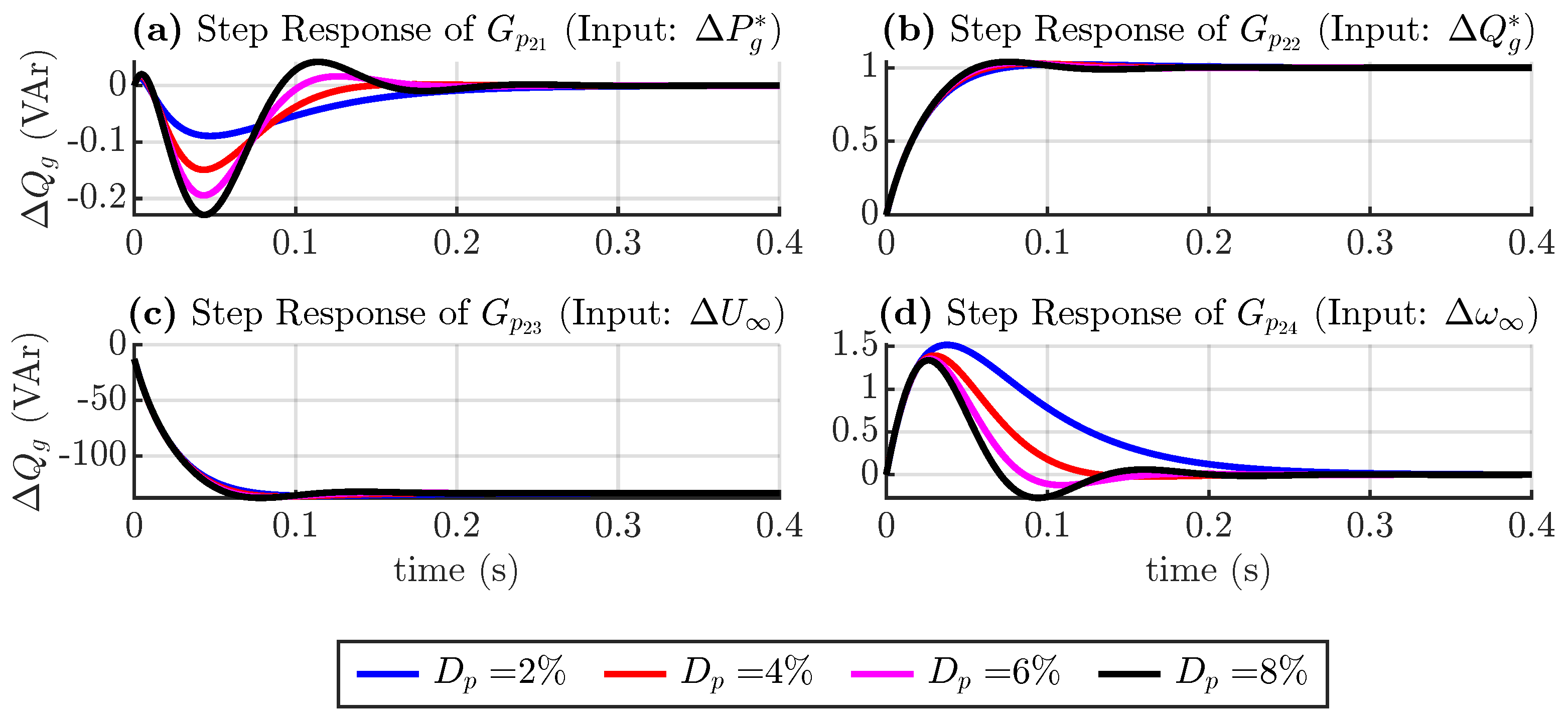
3.2. Reactive Power Loop
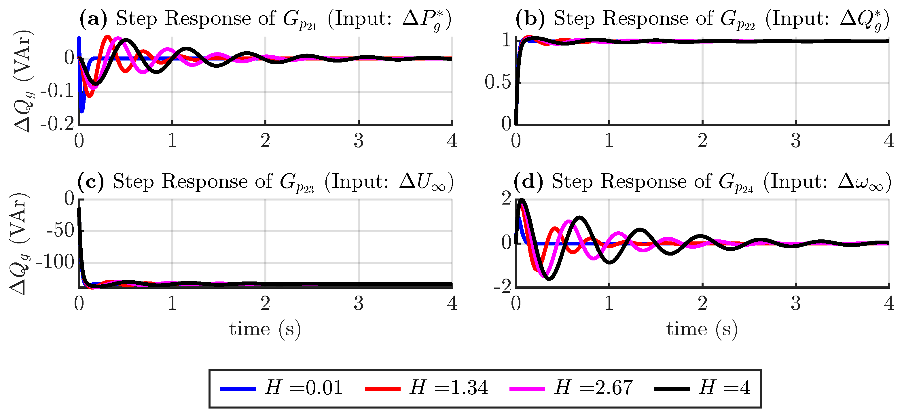
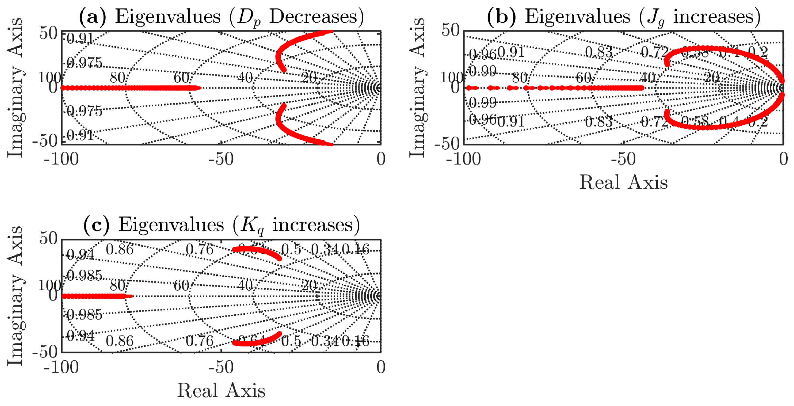
3.3. Root Locus Analysis
4. Maximum Power Point Tracking Method
4.1. Solar Cell Model
4.2. MPPT with Measurements Cells
5. Results
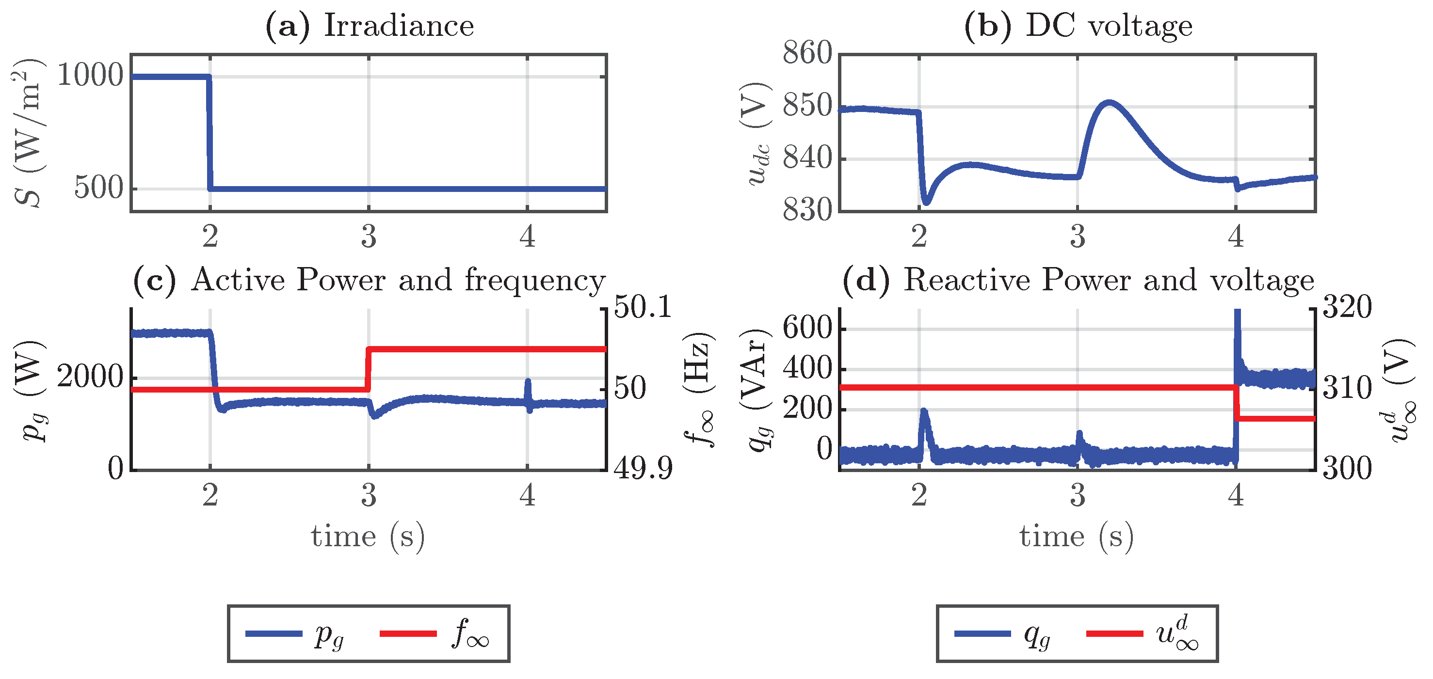
5.1. Simulation Results
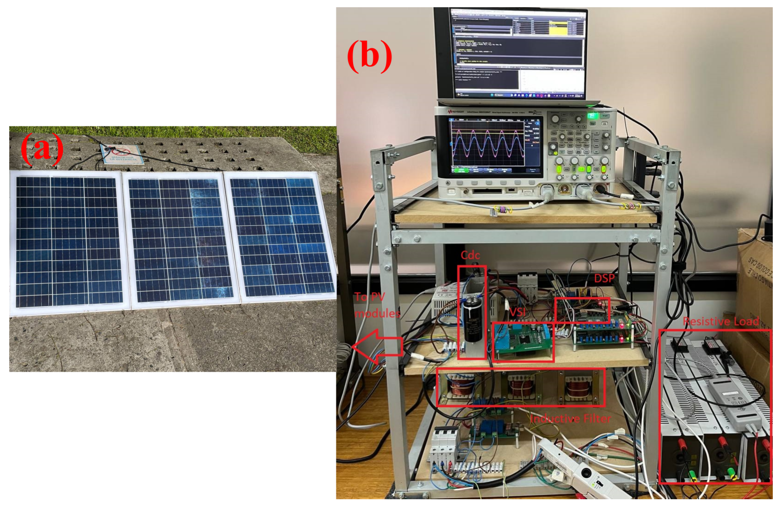
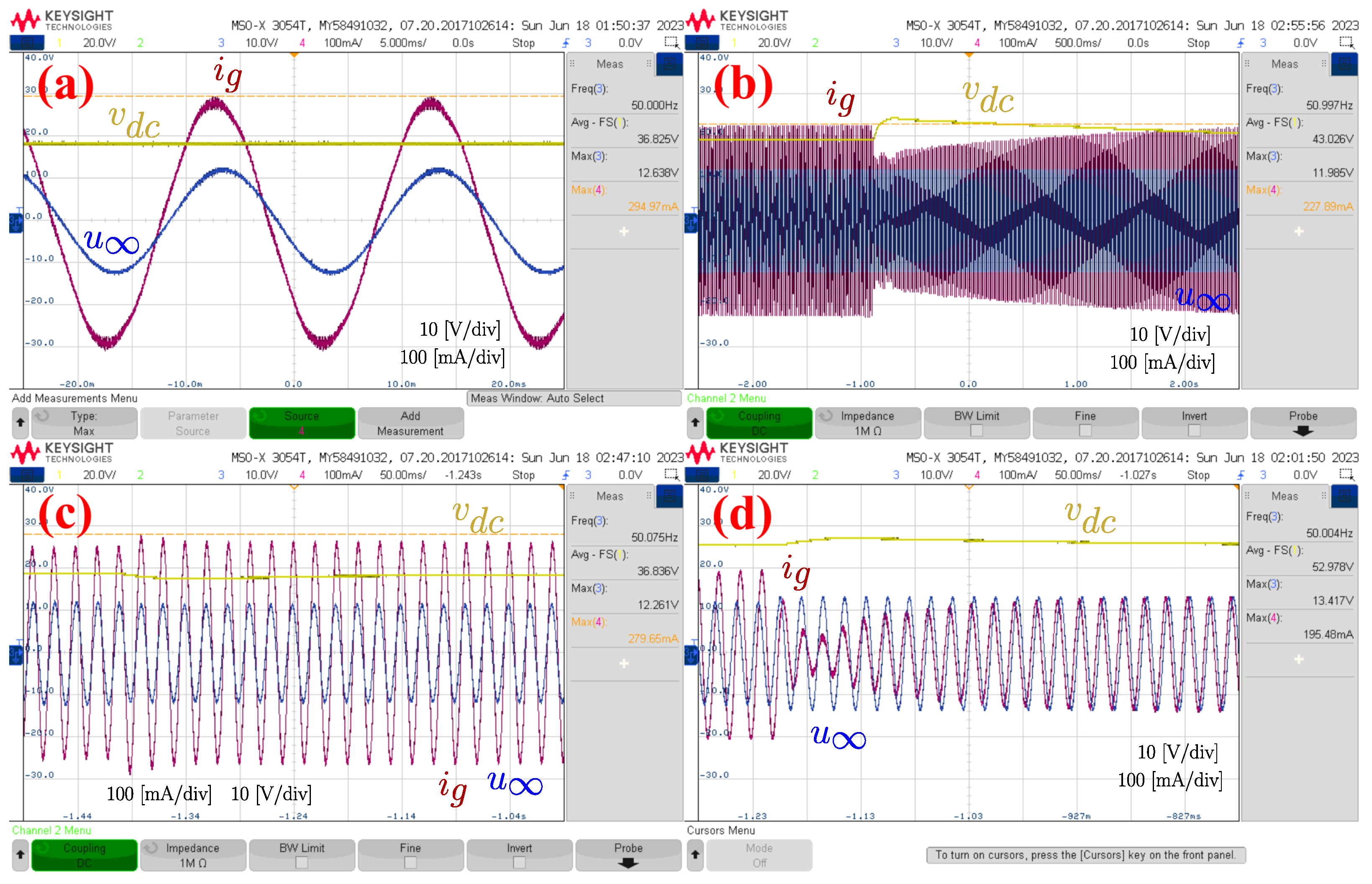
5.2. Experimental Results
5.3. Comparison with Other Works
6. Conclusions
Author Contributions
Funding
Institutional Review Board Statement
Informed Consent Statement
Data Availability Statement
Conflicts of Interest
Abbreviations
| PV | photovoltaic |
| DC | direct current |
| FACTS | flexible AC transmission system |
| MPPT | maximum power point tracking |
Appendix A
References
- Arantegui, R.L.; Jäger-Waldau, A. Photovoltaics and wind status in the European Union after the Paris Agreement. Renew. Sustain. Energy Rev. 2018, 81, 2460–2471. [Google Scholar] [CrossRef]
- O’Connell, B.; Davies, C.; Paver, A.; Taylor, E.; Veijalainen, T.; Ganguli, R.; Schaefer, C. Achieving world-leading penetration of renewables: The australian national electricity market. IEEE Power Energy Mag. 2021, 19, 18–28. [Google Scholar] [CrossRef]
- Badrzadeh, B.; Modi, N.; Lindley, J.; Jalali, A.; Lu, J. Power system operation with a high share of inverter-based resources: The australian experience. IEEE Power Energy Mag. 2021, 19, 46–55. [Google Scholar] [CrossRef]
- Gandhi, O.; Kumar, D.S.; Rodríguez-Gallegos, C.D.; Srinivasan, D. Review of power system impacts at high PV penetration Part I: Factors limiting PV penetration. Sol. Energy 2020, 210, 181–201. [Google Scholar] [CrossRef]
- Hu, J.; Li, Z.; Zhu, J.; Guerrero, J.M. Voltage stabilization: A critical step toward high photovoltaic penetration. IEEE Ind. Electron. Mag. 2019, 13, 17–30. [Google Scholar] [CrossRef]
- Ismael, S.M.; Aleem, S.H.A.; Abdelaziz, A.Y.; Zobaa, A.F. State-of-the-art of hosting capacity in modern power systems with distributed generation. Renew. Energy 2019, 130, 1002–1020. [Google Scholar] [CrossRef]
- Haque, M.M.; Wolfs, P. A review of high PV penetrations in LV distribution networks: Present status, impacts and mitigation measures. Renew. Sustain. Energy Rev. 2016, 62, 1195–1208. [Google Scholar] [CrossRef]
- Anzalchi, A.; Sundararajan, A.; Moghadasi, A.; Sarwat, A. High-penetration grid-tied photovoltaics: Analysis of power quality and feeder voltage profile. IEEE Ind. Appl. Mag. 2019, 25, 83–94. [Google Scholar] [CrossRef]
- Wang, L.; Yan, R.; Saha, T.K. Voltage regulation challenges with unbalanced PV integration in low voltage distribution systems and the corresponding solution. Appl. Energy 2019, 256, 113927. [Google Scholar] [CrossRef]
- Chaudhary, P.; Rizwan, M. Voltage regulation mitigation techniques in distribution system with high PV penetration: A review. Renew. Sustain. Energy Rev. 2018, 82, 3279–3287. [Google Scholar] [CrossRef]
- Kumar, D.S.; Gandhi, O.; Rodríguez-Gallegos, C.D.; Srinivasan, D. Review of power system impacts at high PV penetration Part II: Potential solutions and the way forward. Sol. Energy 2020, 210, 202–221. [Google Scholar]
- Kraiczy, M.; Wang, H.; Schmidt, S.; Wirtz, F.; Braun, M. Reactive power management at the transmission–distribution interface with the support of distributed generators—A grid planning approach. IET Gener. Transm. Distrib. 2018, 12, 5949–5955. [Google Scholar] [CrossRef]
- Tofighi-Milani, M.; Fattaheian-Dehkordi, S.; Fotuhi-Firuzabad, M.; Lehtonen, M. Distributed reactive power management in multi-agent energy systems considering voltage profile improvement. IET Gener. Transm. Distrib. 2023, 17, 4891–4906. [Google Scholar] [CrossRef]
- Guerrero, J.; Gebbran, D.; Mhanna, S.; Chapman, A.C.; Verbič, G. Towards a transactive energy system for integration of distributed energy resources: Home energy management, distributed optimal power flow, and peer-to-peer energy trading. Renew. Sustain. Energy Rev. 2020, 132, 110000. [Google Scholar] [CrossRef]
- Gasperic, S.; Mihalic, R. Estimation of the efficiency of FACTS devices for voltage-stability enhancement with PV area criteria. Renew. Sustain. Energy Rev. 2019, 105, 144–156. [Google Scholar] [CrossRef]
- Varma, R.K.; Siavashi, E.M. PV-STATCOM: A new smart inverter for voltage control in distribution systems. IEEE Trans. Sustain. Energy 2018, 9, 1681–1691. [Google Scholar] [CrossRef]
- Varma, R.K.; Siavashi, E.M.; Mohan, S.; Vanderheide, T. First in Canada, night and day field demonstration of a new photovoltaic solar-based flexible AC transmission system (FACTS) Device PV-STATCOM for stabilizing critical induction motor. IEEE Access 2019, 7, 149479–149492. [Google Scholar] [CrossRef]
- Varma, R.K.; Siavashi, E.; Mohan, S.; McMichael-Dennis, J. Grid support benefits of solar PV systems as STATCOM (PV-STATCOM) through converter control: Grid integration challenges of solar PV power systems. IEEE Electrif. Mag. 2021, 9, 50–61. [Google Scholar] [CrossRef]
- Criollo, A.; Minchala-Avila, L.I.; Benavides, D.; Arévalo, P.; Tostado-Véliz, M.; Sánchez-Lozano, D.; Jurado, F. Enhancing Virtual Inertia Control in Microgrids: A Novel Frequency Response Model Based on Storage Systems. Batteries 2024, 10, 18. [Google Scholar] [CrossRef]
- Muftau, B.; Fazeli, M. The role of virtual synchronous machines in future power systems: A review and future trends. Electr. Power Syst. Res. 2022, 206, 107775. [Google Scholar] [CrossRef]
- Zhong, Q.C.; Weiss, G. Synchronverters: Inverters that mimic synchronous generators. IEEE Trans. Ind. Electron. 2010, 58, 1259–1267. [Google Scholar] [CrossRef]
- Zhong, Q.C.; Nguyen, P.L.; Ma, Z.; Sheng, W. Self-synchronized synchronverters: Inverters without a dedicated synchronization unit. IEEE Trans. Power Electron. 2013, 29, 617–630. [Google Scholar] [CrossRef]
- Dong, S.; Chen, Y.C. Adjusting synchronverter dynamic response speed via damping correction loop. IEEE Trans. Energy Convers. 2016, 32, 608–619. [Google Scholar] [CrossRef]
- Busada, C.A.; Jorge, S.G.; Solsona, J.A. Feedback linearization of a grid-tied synchronverter. IEEE Trans. Ind. Electron. 2022, 70, 147–154. [Google Scholar] [CrossRef]
- Sonawane, A.J.; Umarikar, A.C. Three-phase single-stage photovoltaic system with synchronverter control: Power system simulation studies. IEEE Access 2022, 10, 23408–23424. [Google Scholar] [CrossRef]
- Takamatsu, T.; Oozeki, T.; Orihara, D.; Kikusato, H.; Hashimoto, J.; Otani, K.; Matsuura, T.; Miyazaki, S.; Hamada, H.; Miyazaki, T. Simulation Analysis of Issues with Grid Disturbance for a Photovoltaic Powered Virtual Synchronous Machine. Energies 2022, 15, 5921. [Google Scholar] [CrossRef]
- Perez, M.A.; Espinoza, J.R.; Torres, M.A.; Araya, E.A. A robust PLL algorithm to synchronize static power converters with polluted ac systems. In Proceedings of the IECON 2006—32nd Annual Conference on IEEE Industrial Electronics, Paris, France, 6–10 November 2006; IEEE: Piscataway, NJ, USA, 2006; pp. 2821–2826. [Google Scholar]
- Cavers, J.K.; Mehrotra, K.; Woodward, G.K. Advantages of Second-Order Cartesian Feedback Linearizers for Radio Amplifiers. IEEE Trans. Circuits Syst. I Regul. Pap. 2019, 66, 4134–4146. [Google Scholar] [CrossRef]
- Mehta, H.K.; Warke, H.; Kukadiya, K.; Panchal, A.K. Accurate expressions for single-diode-model solar cell parameterization. IEEE J. Photovolt. 2019, 9, 803–810. [Google Scholar] [CrossRef]
- Morales, R.; Garbarino, M.; Muñoz, J.; Baier, C.; Rohten, J.; Esparza, V.; Dewar, D. Grid connected PV system with new MPPT estimation method based on measuring cells. In Proceedings of the IECON 2019—45th Annual Conference of the IEEE Industrial Electronics Society, Lisbon, Portugal, 14–17 October 2019; IEEE: Piscataway, NJ, USA, 2019; Volume 1, pp. 2366–2371. [Google Scholar]
- Silva, J.J.; Rohten, J.A.; Villarroel, F.A.; Pulido, E.S.; Rivera, M.E. A Honeycomb-Like Predictive Controller With a Reduced Computational Burden for Three-Level NPC Converters. IEEE Trans. Power Electron. 2024, 39, 2051–2062. [Google Scholar] [CrossRef]


| Parameter | Value | Parameter | Value |
|---|---|---|---|
| 3000 VA | 380 VRMS | ||
| 50 Hz | 48.13 | ||
| 1 | 10 mH | ||
| 60 W | 2.35 mF | ||
| PV modules | 50 | H | 0.4 s |
| PV strings | 1 | 3.039 Nms/rad | |
| PV | 21.1 V | 96.77 VAr/V | |
| PV | 3.8 A | 1000 VAr/V | |
| PV | 17.1 V | 0.009 | |
| PV | 3.5 A | 4 | |
| 20 kHz |
| Inverter Parameters | Value | PV Parameters | Value |
|---|---|---|---|
| 100 VA | 15 VRMS | ||
| Module number | 3 | 21.71 V | |
| 0.25 | 2.92 A | ||
| 3.7 mH | 18.2 V | ||
| 2.35 mF | 2.78 A |
Disclaimer/Publisher’s Note: The statements, opinions and data contained in all publications are solely those of the individual author(s) and contributor(s) and not of MDPI and/or the editor(s). MDPI and/or the editor(s) disclaim responsibility for any injury to people or property resulting from any ideas, methods, instructions or products referred to in the content. |
© 2024 by the authors. Licensee MDPI, Basel, Switzerland. This article is an open access article distributed under the terms and conditions of the Creative Commons Attribution (CC BY) license (https://creativecommons.org/licenses/by/4.0/).
Share and Cite
Albornoz, M.; Rohten, J.; Espinoza, J.; Varela, J.; Sbarbaro, D.; Gallego, Y. Photovoltaic Power Injection Control Based on a Virtual Synchronous Machine Strategy. Sensors 2024, 24, 4039. https://doi.org/10.3390/s24134039
Albornoz M, Rohten J, Espinoza J, Varela J, Sbarbaro D, Gallego Y. Photovoltaic Power Injection Control Based on a Virtual Synchronous Machine Strategy. Sensors. 2024; 24(13):4039. https://doi.org/10.3390/s24134039
Chicago/Turabian StyleAlbornoz, Miguel, Jaime Rohten, José Espinoza, Jorge Varela, Daniel Sbarbaro, and Yandi Gallego. 2024. "Photovoltaic Power Injection Control Based on a Virtual Synchronous Machine Strategy" Sensors 24, no. 13: 4039. https://doi.org/10.3390/s24134039