Abstract
Conventional air quality monitoring networks typically tend to be sparse over areas of interest. Because of the high cost of establishing such monitoring systems, some areas are often completely left out of regulatory monitoring networks. Recently, a new paradigm in monitoring has emerged that utilizes low-cost air pollution sensors, thus making it possible to reduce the knowledge gap in air pollution levels for areas not covered by regulatory monitoring networks and increase the spatial resolution of monitoring in others. The benefits of such networks for the community are almost self-evident since information about the level of air pollution can be transmitted in real time and the data can be analysed immediately over the wider area. However, the accuracy and reliability of newly produced data must also be taken into account in order to be able to correctly interpret the results. In this study, we analyse particulate matter pollution data from a large network of low-cost particulate matter monitors that was deployed and placed in outdoor spaces in schools in central and western Serbia under the Schools for Better Air Quality UNICEF pilot initiative in the period from April 2022 to June 2023. The network consisted of 129 devices in 15 municipalities, with 11 of the municipalities having such extensive real-time measurements of particulate matter concentration for the first time. The analysis showed that the maximum concentrations of PM2.5 and PM10 were in the winter months (heating season), while during the summer months (non-heating season), the concentrations were several times lower. Also, in some municipalities, the maximum values and number of daily exceedances of PM10 (50 μg/m3) were much higher than in the others because of diversity and differences in the low-cost sensor sampling sites. The particulate matter mass daily concentrations obtained by low-cost sensors were analysed and also classified according to the European AQI (air quality index) applied to low-cost sensor data. This study confirmed that the large network of low-cost air pollution sensors can be useful in providing real-time information and warnings about higher pollution days and episodes, particularly in situations where there is a lack of local or national regulatory monitoring stations in the area.
1. Introduction
Air pollution, including both particulate matter (PM) and gas-phase pollutants, continues to be a worldwide hot topic since it is associated with various negative effects on human health []. Outdoor air pollution, consisting of gaseous pollutants and particulate matter, was designated by the International Agency for Cancer Risk (IARC) as a Group 1 carcinogenic substance, i.e., proven human carcinogen []. Ambient PM was also evaluated, independently of gas-phase pollutants, and classified as a Group 1 carcinogenic substance []. In most counties, National Air Quality Standards for main ambient pollutants are much higher than the WHO Air Quality Guidelines values [].
Air pollution is a complex phenomenon, originating from multiple anthropogenic and natural sources. Anthropogenic sources include vehicular transport, domestic heating, energy generation, and industrial production. This highlights the need for improvements in monitoring air pollution because of its highly variable spatial and temporal patterns. National and local air quality monitoring networks monitor and measure air pollutants by methods with prescribed accuracy and precision, using high-end monitors and sophisticated quality assurance and quality control systems that are very expensive to establish, run, and maintain. This ensures comparability of measurements across different geographical areas and meteorological and climatic conditions. The number of air quality monitoring stations is limited because of the high price of reference- and equivalence-grade monitors and the high costs of qualified personnel that perform monitoring and maintain instruments. However, for personalized information, it is necessary to have access to air quality data with higher temporal and spatial resolution. Over the past decade, both the scientific community and citizens have recognized the great potential of the emerging paradigm of low-cost (LC) air quality sensors and documented the pros and cons of their use [,]. These sensors are small in size, modest in price, easy to handle, have fast response [], and can be relatively easily deployed in a dense sensor network. This improves the spatial resolution of AQ measurements as they are widespread over cities [,,], suburban [] and rural areas, larger spaces [,], and hard-to-reach areas [,,,], which is their clear advantage over automatic monitoring stations. However, the performance of low-cost sensors needs to be carefully monitored as it can vary from sensor to sensor, which makes it necessary to examine the data quality of each node both during continuous use and before deployment []. Additionally, performance can vary spatially and over longer periods of time, as it depends on both short- and long-term exposure of the sensor to various environmental influences such as atmospheric composition and meteorological conditions []. Some of these performance issues can be alleviated by using a larger number of sensors connected in a network and applying methods and principles of sensor network metrology []. In this way, larger, richer, and more open data information can be obtained and used not only for mapping the pollutants but also for identifying sources, tracking changes, and predicting extreme air quality events [].
The application of low-cost air quality monitoring networks has substantially grown over the last decade because of technological advances in the production of cheap and portable air pollution sensors [,,,,,]. Recent review papers [,] analysed practical aspects of outdoor air quality low-cost sensor networks, focusing on gas pollutant networks (analysed a total of 60 LCS networks targeting outdoor environments all over the world) and Carotenuto et al. [] including both gas and PM sensor networks. In the open-access literature, Carotenuto et al. identified a total of 111 low-cost air quality monitoring networks for campaigns that had a duration from 3 months up to 4 years that were performed in the period 2014–2022. In the framework of AQ low-cost sensor networks, the most represented was atmospheric pollution of particulate matter fractions PM10 (13.3%), PM2.5 (41.2%), and PM1 (2.2%). The networks mainly consisted of 3–10 devices (52 LCS networks) and 10–100 devices (50 LCS networks), and only 7 had 100–500 nodes, with 2 networks having more than 2000 nodes []. Based on these results, it can be concluded that this puts a network built under the UNICEF initiative into a group of the 10% largest LCS network studies.
Sensor networks, when deployed with a sufficient number of nodes, increase the often-limited spatial information on air quality conditions provided by conventional monitoring networks. However, the use of low-cost air quality sensors still has many limitations, mostly related to the reliability of their measurements and quality control of the large amount of data they provide []. Thus, to deploy a large-scale sensor network and meaningfully use the generated data, it is important to formulate standard operating procedures for assessing the short- and long-term performance of low-cost sensors and performance metrics that supplement the reported measurement results []. In addition, different approaches to evaluating data from low-cost sensors in air quality models have been proposed to increase spatial and temporal resolution [,,]. It is also important to strike the right balance between network size and cost of calibration since if the network is too dense, the cost of calibration and maintenance can quickly become much larger than the initial cost of installation, thus defeating its original purpose. Therefore, the data have to be as accurate as they can, without the need for regular on-site calibration, because the necessary network scale may be very large, containing hundreds or more instruments [,]. Last, but not least important, the goal of such measurements is to engage communities in identifying concerns and solutions that can support adequate decision-making by institutions responsible for air quality control [].
In this study, we present the results of a low-cost sensor network implementation that includes 43 locations in 15 municipalities in central and western Serbia in the period from 1 April 2022 to 30 June 2023. Before deployment in schools across the 15 municipalities, all sensors passed the procedure of collocation calibration at the automatic monitoring station. We also show daily PM2.5 and PM10 episodes and compare them with the Serbian Environmental Protection Agency (SEPA) open data for 4 out of the 15 municipalities in which automatic stations equipped with PM monitors exist.
2. Materials and Methods
2.1. Low-Cost Sensor Network
The sensor network, established under the “Schools for Better Air Quality” UNICEF Serbia pilot initiative, used a low-cost sensor node equipped with a PMS7003 air dust sensor for measurements of particulate matter fractions (PM10, PM2.5 and PM1), with a node specifically developed in the framework of the UNICEF initiative. As reported in a number of publications, the PMS7003 sensor has been successfully used for the detection of PM10, PM2.5, and PM1 in indoor and outdoor environments. PMS7003 belongs to the family of Plantower models (PMS1003, PMS3003, PMS5003, PMS7003, and PMS-A003) that have lower prices compared with other low-cost PM sensors with similar characteristics [,,,]. UNICEF nodes upload data into the cloud backend, calibration coefficients are applied at the server side, and near real-time data about air quality is made publicly available on a dedicated website.
The low-cost sensor network consisted of 129 devices at 43 locations in 15 municipalities in central and western Serbia (the basins of two rivers including Velika Morava and Zapadna Morava), as shown in Figure 1a, including Užice (M1), Kraljevo (M2), Kruševac (M3), Čačak (M4), Gornji Milanovac (M5), Novi Pazar (M6), Raška (M7), Kosjerić (M8), Loznica (M9), Osečina (M10), Priboj (M11), Bajina Bašta (M12), Bogatić (M13), Nova Varoš (M14), and Prijepolje (M15). Network nodes were made in the framework of the UNICEF initiative, equipped with low-cost OPS (Plantower PMS7003), and deployed in each of the 15 municipalities (in three schools in 11, in two schools in 3, and in four schools in 1 of the municipalities). We analysed the data set acquired in the period from April 2022 to June 2023. To ensure uninterrupted reporting, reliability was increased by adding redundant nodes, i.e., three nodes with PM sensors placed at each of the measuring sites (location) measured particulate matter pollution in the outdoor school environment (Figure 1b).
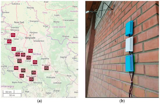
Figure 1.
(a) Map of Serbia with the position of 15 municipalities that participated in this study. (b) An example of low-cost sensor positioning at one of the measuring sites. Note the redundant nodes, which increase the reliability of the network.
The protocol for the outdoor placement of network nodes at schools had the following requirements: not to face a traffic-dense street or a parking lot that would interfere with the measurements in irregular intervals; not to be in the immediate vicinity of trees that would locally reduce air pollution; and not to be at the height above the first-floor level.
The performance metrics of the sensor nodes were checked by periodic calibration, the details of which can be found in Appendix A. After each calibration, coefficients and measurement uncertainties were obtained and quantified by Root Mean Square Error (RMSE) [], which was an average of 6.50 µg/m3 and 12.95 µg/m3 after initial calibration for PM2.5 and PM10, respectively. Parameters of linear calibration for every sensor were calculated from measured values for the period when low-cost sensors were collocated near the SEPA automatic monitoring station equipped with a Grimm EDM 180 equivalence PM monitor. Average hourly values were obtained according to minute values from all available sensors from one school. It was necessary to have a data coverage of 75% for an hourly datapoint to be valid. Similarly, a data coverage of 75% was needed to obtain a valid daily average.
2.2. Comparison with Data from the State AQ Monitoring Network
In this study, hourly PM10 and PM2.5 data were obtained via the State Network run by the Serbian Environmental Protection Agency (SEPA), http://www.amskv.sepa.gov.rs/ (accessed on 19 August 2023). Automatic monitoring stations belonging to the State AQ Monitoring Network equipped with Grimm EDM 180 monitor exist in 4 out of the 15 municipalities in which low-cost sensors are located as follows: M1, M4, M6, and M8. The maps of SEPA and low-cost sensor sites are given in Figure 2, and Table 1 presents the distance of each school from the SEPA location in each of these four cities. The simultaneous data obtained from SEPA and the low-cost sensors are available for the period of May 2022–June 2023.
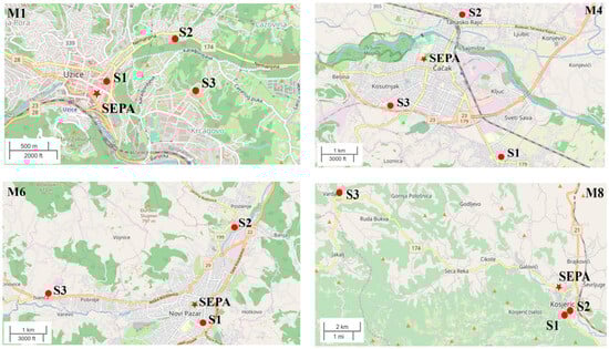
Figure 2.
Maps of low-cost sensor locations and SEPA for municipalities M1, M4, M6, and M8. Points present schools and stars present SEPA locations.

Table 1.
Distances of low-cost sensor locations from SEPA stations in four cities.
3. Results and Discussion
3.1. PM2.5 and PM10 Measurements by SEPA Stations and Low-Cost Sensor Networks
During the campaign, data derived from the low-cost PM sensors were compared with the results obtained from the SEPA air quality monitoring station. Time series plots for the SEPA station and each low-cost sensor location within each municipality are provided in Figure 3 and Figure 4. They show how low-cost time series (lines in colours) vary in relation to the data from the SEPA instrument (dashed black line). In general, the concentrations of PM10 as well as PM2.5 are elevated during the winter months. As can be seen in Figure 3, the exceedances of PM10 over 50 µg/m3 occur during the period October 2022–January 2023, but for M1, they occur during the whole period. The maximum concentration of PM10 was in M6, reaching over 350 µg/m3. The time series for PM2.5 also show large values for M1 and M4, with maximums of more than 200 µg/m3.
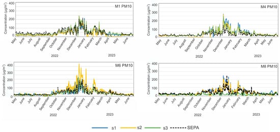
Figure 3.
Time series of hourly PM10 data reported for each of the community monitoring locations over the study period. SEPA data are presented as a dashed black colour, and data from schools s1, s2, and s3 are presented as blue, yellow, and green, respectively.
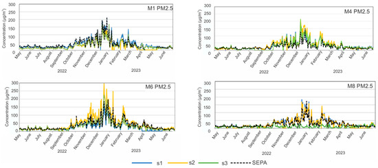
Figure 4.
Time series of hourly PM2.5 data reported for each of the low-cost monitoring locations over the study period. SEPA data are presented as a dashed black colour, and data from schools s1, s2, and s3 are presented as blue, yellow, and green, respectively.
For each of the four municipalities with SEPA stations, we can compare the PM10 and PM2.5 concentrations to those obtained with low-cost sensor networks at three locations in every city. For M1, the SEPA results are in agreement with those obtained by the low-cost sensors at all three locations (locations can be seen in Figure 1), even if some locations are around 1 km from SEPA. On the other hand, for municipalities M4 and M6, during the heating season, SEPA showed much lower PM10 concentrations than the low-cost sensors (max difference of around 200 µg/m3). For M4, the SEPA station is in the urban area of the city and the other three locations are more than 1.5 km away from the SEPA station (Figure 1). For M6, the measured levels have similar trends; however, at one of the sites (s2), the concentration reported by the LCS network is much higher than SEPA and the other sites in M6, potentially indicating a strong local influence of individual heating. At M8, two locations of low-cost sensors are in agreement with the SEPA results, but one location displayed totally different PM10 results because it is far away from the urban area. Similar results can be seen for PM2.5 in Figure 4, while for M1 low-cost sensors, the data are in the best agreement with SEPA. In addition, it can be observed that in all four municipalities, a better agreement between low-cost sensors and SEPA occurs at lower concentrations, indicating better sensor performance for lower PM concentrations.
3.2. PM10 and PM2.5 Measurements by Low-Cost Sensor Networks
The averaged time series for PM10 and PM2.5 across the whole measured period in every municipality within the low-cost sensor network are displayed in Figure 5 and Figure 6. They indicate that the concentrations of PM10 and PM2.5 are much higher during the heating season—October 2022 to April 2023.
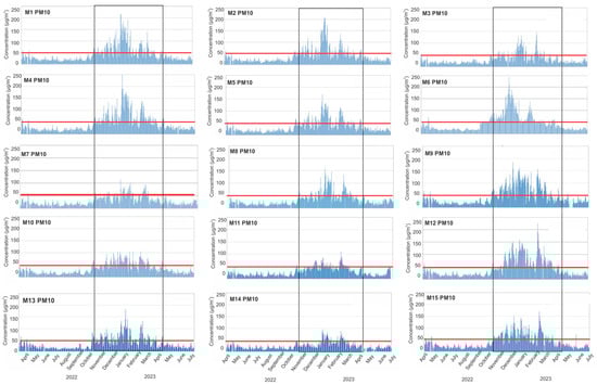
Figure 5.
Time series of hourly PM10 data averaged per three (most commonly) measurement sites within the municipality over the study period. Grey rectangles represent the heating season, and the red line is the limit for PM10 of 50 µg/m3.
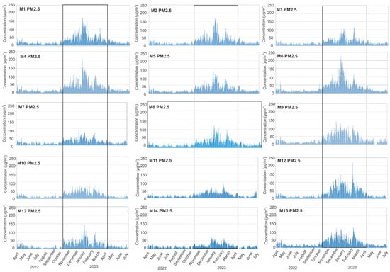
Figure 6.
Time series of hourly PM2.5 data averaged per three (mostly) measurement sites within the municipality over the study period. Grey rectangles represent the heating season.
The exceedances of PM10 concentrations over 50 µg/m3 occur during the heating period October 2022–April 2023 in almost all municipalities (see Figure 5). The maximum concentrations can be seen in municipalities M1, M2, and M4, where they were more than 200 µg/m3 during the winter months. On the other hand, during the summer months, there were almost no days of exceedance.
When we observe the time series for PM2.5, the maximum concentrations occur in M1, M4, M6, and M12 during the winter months (Figure 6) when the mass concentrations were over 200 µg/m3 for one or two days. The smallest values of PM2.5 are in M7, M10, M11, and M14, which is probably associated with locations where sensors collected PMs in rural areas, similar to PM10 concentrations in these municipalities.
For an indication of the current status of urban air pollution, the European Air Quality Index (AQI) [] was used. We calculated the percentage of days during the examined period according to each category as follows:
- PM10: very good 0–20 µg/m3; good 20–40 µg/m3; medium 40–50 µg/m3; poor 50–100 µg/m3; very poor 100–150 µg/m3; and extremely poor 150–1200 µg/m3.
- PM2.5: very good 0–10 µg/m3; good 10–20 µg/m3; medium 20–25 µg/m3; poor 25–50 µg/m3; very poor 50–75 µg/m3; and extremely poor 75–800 µg/m3.
Figure 7 shows the percentage of days during the whole period (April 2022–June 2023) of every AQI category in each city.
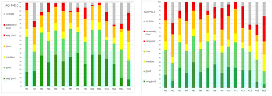
Figure 7.
Percentage of days with each of the 6 AQI categories for PM10 and PM2.5 in all 15 municipalities.
Poor-extremely poor AQI for PM10 was detected in the range of 1 to 21% of days. The highest value of poor-extremely poor air was in municipality M15, and only 1% of such highly polluted days occurred in M7. Poor-extremely poor AQI for PM2.5 was detected in the range of 5 to 30% of days, while in 3/15 municipalities, i.e., M9, M12, and M1, it was in the range of 25–30% of days.
However, very good-good PM10 values were all in the range of 31–69% of days, with more than 60% of days in 6/15 municipalities (M3, M5, M7, M8, M10, and M11), while 31% of days, which was the lowest number of days, was identified in M15. Regarding AQI for PM2.5, for very good–good, it varied through municipalities in the range from 19% to 60% of days, the lowest observed in M15 and the highest in M5. In 5/15 municipalities, more than 50% of days were in the very good–good AQI PM2.5.
In Figure 8, pie charts are given for one of the most polluted cities, Prijepolje (M15), located at the River Lim surrounded by mountains, and one of the less polluted cities, Kruševac (M3), which is in the valley of Zapadna Morava River, according to the analysis of AQI categories of PMs for 15 months (6 months of heating and 9 months of non-heating).
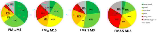
Figure 8.
Pie charts with the percentage of days for each of the 6 AQI categories for PM10 and PM2.5 in M3 and M15.
With this study, we confirmed that having monitoring sites equipped even with low-cost sensor devices in one municipality can help to identify PM daily concentrations, pollution episodes, and even diurnal variations, especially in cities in which there is no PM monitoring in the framework of a state or local monitoring network. For instance, municipalities M12, M11, and M10 have a large percentage of days with poor AQI categories for PM10 and PM2.5, and in these municipalities, there are no automatic monitoring stations.
An important aspect of this kind of study is the ability of low-cost sensors to provide the public with more immediate and relevant information via websites and services that can warn individuals when air pollution levels are above thresholds. The outcome of this study can raise the awareness of citizens and local authorities about PM pollution and the necessity for performing more studies, online monitoring, and modelling in the 15 municipalities that participated in this study.
4. Conclusions
In this study, a large network of low-cost particulate matter monitors was deployed at 43 locations in 15 municipalities in central and western Serbia, which measured PM10 and PM2.5 for a period of 15 months, from April 2022 to June 2023. In almost all the municipalities, the main source of pollution is individual heating and associated facilities, while in a few municipalities, there are well-known industrial activities. Traffic intensity also contributes in some sites where the diffusion of pollution is hindered by local orography.
Based on the time series of PM concentration in municipalities 1 and 4, which have both SEPA and low-cost sensor PM monitors, we concluded that the levels for PM2.5 and PM10 are comparable to the SEPA results and are generally very similar across schools in the same municipality, with some exceptions, which are due to the presence of strong local sources or differences in population densities between urban and rural areas. In all 15 municipalities, the maximum concentrations of PM2.5 and PM10 were observed in the winter season, while during the summer months, the PM concentrations were significantly lower. In almost all municipalities, the most polluted months were December and/or January. PM10 24 h concentration in each municipality exceeded limit values of 50 µg/m3.
Looking at the distributions of AQI categories of PMs for the whole period, the highest percentage of poor–extremely poor AQI were in M7 and M12 for PM10 and in M1, M4, M6, and M7 for PM2.5. On the other hand, very good to medium AQI PM10 values were the highest in M10 and M11, while for PM2.5, they were best in M5 and M11.
The significant result of this study is the ability of low-cost sensors to provide the public with more information about air pollution levels, especially in municipalities where offline and online monitoring of PM10 and PM2.5 within local- and state-level networks does not exist. Furthermore, in the UNICEF initiative, the importance of raising awareness about ambient air pollution is one of the main goals. Furthermore, since sensors were placed in the outdoor micro-environment, this study has hopefully helped in raising the awareness of school children about this topic.
Author Contributions
Conceptualization, D.B.S.; methodology, D.B.S., D.K., M.D., M.Ž., U.R., M.J., I.L., and M.J.-S.; validation, D.K. and M.D.; formal analysis, D.B.S., M.D., and M.J.-S.; investigation, D.B.S.; writing—original draft preparation, D.B.S., D.K., and M.J.-S.; writing—review and editing, D.B.S., M.D., and M.J.-S.; supervision, M.J.-S.; project administration, M.J.-S.; funding acquisition, M.J.-S. All authors have read and agreed to the published version of the manuscript.
Funding
This research was funded by: The European Union’s Horizon Europe Research and Innovation Program under GA 952433, H2020 VIDIS project; The Government of Norway and implemented by UNICEF initiative “Schools for Better Air Quality: Citizens-Based Monitoring, STEM Education, and Youth Activism in Serbia”; the Ministry of Education, Science and Technological Development of the Republic of Serbia under GA 451-03-47/2023-01/200017.
Institutional Review Board Statement
Not applicable.
Informed Consent Statement
Not applicable.
Data Availability Statement
Data are contained within the article.
Acknowledgments
We acknowledge to Faculty of Technical Sciences Čačak, University of Kragujevac for logistic support during the second colocation campaign.
Conflicts of Interest
The authors declare no conflict of interest.
Appendix A
Before deployment in the 15 municipalities, all sensor network nodes were subject to an extensive collocation campaign that was conducted at the SEPA station in Belgrade and lasted for 3 weeks (4–28 February 2022). Summary statistics of the meteorological and air pollution conditions during the collocation campaign are given in Table A1.
Table A1.
Summary statistics of the meteorological and air pollution conditions during the first collocation campaign, SEPA station Belgrade, 4–28 February 2022.
Table A1.
Summary statistics of the meteorological and air pollution conditions during the first collocation campaign, SEPA station Belgrade, 4–28 February 2022.
| PM1 [μg/m3] | PM2.5 [μg/m3] | PM10 [μg/m3] | SO2 [μg/m3] | NO2 [μg/m3] | T [°C] | RH [%] | |
|---|---|---|---|---|---|---|---|
| 2nd perc. | 2.79 | 3.50 | 4.63 | 3.16 | 7.95 | 2.29 | 33.23 |
| 98th perc. | 86.30 | 90.36 | 118.24 | 27.14 | 123.21 | 17.20 | 89.63 |
| mean | 22.03 | 24.68 | 35.02 | 9.98 | 50.88 | 8.23 | 62.04 |
| median | 16.28 | 19.08 | 27.34 | 7.55 | 48.63 | 7.75 | 61.14 |
The calibration coefficients for all sensor nodes were derived based on this initial collocation campaign before deployment []. After that, the sensors were deployed in the 15 municipalities where they produced a calibrated data stream. Box plots of performance metric summary statistics (R2 and RMSE) are given in Figure A1 (denoted as before deployment). Since we used univariate linear regression, the impact of the linear regression term is on the scale of the predictions. Furthermore, the intercept parameter of the linear regression model unifies the response across the sensor fleet in conditions of low pollution.
Recalibration efforts are a needed part of a metrologically sound approach to low-cost sensor network deployment. These recalibration efforts have several purposes. Firstly, since the long-term deployment will span several seasons, calibration coefficients derived during one season could be inadequate for another season. That is why recalibration should be performed once the meteorological conditions have changed significantly. Secondly, sensor performance may degrade over time. It is possible to quantify such drops in performance by performing a new calibration.
The new (re)calibration campaign was conducted in the period from 11 April to 11 May 2023. Summary statistics of the meteorological and air pollution conditions during the (re)calibration collocation campaign are given in Table A2.
Table A2.
Summary statistics of the meteorological and air pollution conditions during the second collocation campaign, SEPA station Čačak, 11 April–11 May 2023.
Table A2.
Summary statistics of the meteorological and air pollution conditions during the second collocation campaign, SEPA station Čačak, 11 April–11 May 2023.
| PM1 [μg/m3] | PM2.5 [μg/m3] | PM10 [μg/m3] | SO2 [μg/m3] | NO2 [μg/m3] | T [°C] | RH [%] | |
|---|---|---|---|---|---|---|---|
| 2nd perc. | / | 3.27 | 4.40 | 5.60 | 3.38 | 4.00 | 30.55 |
| 98th perc. | / | 44.16 | 59.93 | 21.99 | 38.92 | 22.61 | 92.24 |
| mean | / | 15.32 | 21.15 | 8.22 | 11.70 | 13.28 | 64.66 |
| median | / | 13.50 | 18.80 | 6.85 | 9.46 | 13.16 | 68.79 |
Note that the currently accepted best practice is to perform collocation next to the reference station, thus ensuring the traceability of the collocated instrument. However, another requirement was also imposed on the sensor network to ensure uninterrupted continuous reporting. To meet both requirements, the method that was used for calibration was a combination of a collocation method (as used in the initial calibration when it was possible to collocate all available instruments) and a transfer of calibration (in order to transfer the new calibration coefficients to the instrument that were not collocated but instead stayed at the deployment location in order to ensure uninterrupted reporting).
Furthermore, since calibrated devices can be used to transfer calibration, transfer coefficients are also needed. These were calculated based on the most recent month (March 2023) when the devices were collocated at their deployment locations. In summary, for each collocated device, 1-hop calibration and 1-hop transfer coefficients were calculated, as well as 2-hop transfer/calibration coefficients. Here, the term “hop” is used to name a process of a single univariate linear transformation on the data, for which the transformation coefficients were derived using collocation (either between the low-cost sensor and the reference or between the two low-cost sensors). This procedure results in updated coefficients for all LCS nodes in each school, where a collocated unit will have new coefficients obtained via 1-hop linear calibration, and the remaining deployed units will have new coefficients obtained via 2-hop linear calibration, which are obtained by composition of transfer and calibration.
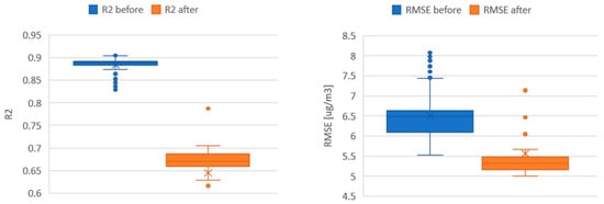
Figure A1.
Summary statistics of the PM2.5 calibration performance of the LCS nodes before deployment (denoted as R2 before and RMSE before) and after (re)calibration (denoted as R2 after and RMSE after).
As illustrated in Figure A1, with the approach to calibration and recalibration used, which is also recommended for low-cost sensor networks by WMO [], it is only possible to observe how the performance changed over the period of the deployment. However, it is not possible to have a more detailed picture of fine/gradual temporal changes in uncertainty.
References
- World Health Organization. Air Quality Guidelines-Update 2021; WHO Regional Office for Europe: Copenhagen, Denmark, 2021. [Google Scholar]
- IARC: Outdoor Air Pollution a Leading Environmental Cause of Cancer Deaths. IARC Press Release. 2013. Available online: http://www.iarc.fr/en/media-centre/pr/2013/pdfs/pr221_E.pdf (accessed on 1 April 2024).
- WHO, National Air Quality Standards. Available online: https://www.who.int/tools/air-quality-standards (accessed on 1 April 2024).
- Jovašević-Stojanović, M.; Bartonova, A.; Topalović, D.; Lazović, I.; Pokrić, B.; Ristovski, Z. On the use of small and cheaper sensors and devices for indicative citizen-based monitoring of respirable particulate matter. Environ. Pollut. 2015, 206, 696–704. [Google Scholar] [CrossRef]
- Giordano, M.R.; Malings, C.; Pandis, S.N.; Presto, A.A.; McNeill, V.F.; Westervelt, D.M.; Beekmann, M.; Subramanian, R. From low-cost sensors to high-quality data: A summary of challenges and best practices for effectively calibrating low-cost particulate matter mass sensors. J. Aerosol Sci. 2021, 158, 105833. [Google Scholar] [CrossRef]
- Idrees, Z.; Zheng, L. Low-cost air pollution monitoring systems: A review of protocols and enabling technologies. J. Ind. Inf. Integr. 2020, 17, 100123. [Google Scholar] [CrossRef]
- Ahangar, F.E.; Frank, R.F.; Akula, V. Using Low-Cost Air Quality Sensor Networks to Improve the Spatial and Temporal Resolution of Concentration Maps. Int. J. Environ. Res. Public Health 2019, 16, 1252. [Google Scholar] [CrossRef]
- Johnston, S.J.; Basford, P.J.; Bulot, F.M.J.; Apetroaie-Cristea, M.; Easton, N.H.C.; Davenport, C.; Foster, G.L.; Loxham, M.; Morris, A.K.; Cox, S.J. City scale particulate matter monitoring using LoRaWAN based air quality IoT devices. Sensors 2019, 19, 209. [Google Scholar] [CrossRef] [PubMed]
- Lu, Y.; Giuliano, G.; Habre, R. Estimating hourly PM2.5 concentrations at the neighborhood scale using a low-cost air sensor network: A Los Angeles case study. Environ. Res. 2021, 195, 110653. [Google Scholar] [CrossRef] [PubMed]
- Jiao, W.; Hagler, G.; Williams, R.; Sharpe, R.; Brown, R.; Garver, D.; Judge, R.; Caudill, M.; Rickard, J.; Davis, M.; et al. Community Air Sensor Network (CAIRSENSE) project: Evaluation of low-cost sensor performance in a suburban environment in the southeastern United States. Atmos. Meas. Tech. 2016, 9, 5281–5292. [Google Scholar] [CrossRef] [PubMed]
- Chao, C.Y.; Zhang, H.; Hammer, M.; Zhan, Y.; Kenney, D.; Martin, R.V.; Biswas, P. Integrating fixed monitoring systems with low-cost sensors to create high-resolution air quality maps for the northern China plain region. ACS Earth Space Chem. 2021, 5, 3022–3035. [Google Scholar] [CrossRef]
- Li, J.; Zhang, H.; Chao, C.-Y.; Chien, C.-H.; Wu, C.-Y.; Luo, C.H.; Chen, L.J.; Biswas, P. Integrating low-cost air quality sensor networks with fixed and satellite monitoring systems to study ground-level PM2.5. Atmos. Environ. 2020, 223, 117293. [Google Scholar] [CrossRef]
- Bisignano, A.; Carotenuto, F.; Zaldei, A.; Giovannini, L. Field calibration of a low-cost sensors network to assess trafficrelated air pollution along the Brenner highway. Atmos. Environ. 2022, 275, 119008. [Google Scholar] [CrossRef]
- Amoah, N.A.; Xu, G.; Wang, Y.; Li, J.; Zou, Y.; Nie, B. Application of low-cost particulate matter sensors for air quality monitoring and exposure assessment in underground mines: A review. Int. J. Miner. Met. Mater. 2022, 29, 1475–1490. [Google Scholar] [CrossRef]
- Zafra-Pérez, A.; Boente, C.; de la Campa, A.S.; Gómez-Galán, J.A.; de la Rosa, J.D. A novel application of mobile low-cost sensors for atmospheric particulate matter monitoring in open-pit mines. Environ. Technol. Innov. 2023, 29, 102974. [Google Scholar] [CrossRef]
- Castell, N.; Dauge, F.R.; Schneider, P.; Vogt, M.; Lerner, U.; Fishbain, B.; Broday, D.; Bartonova, A. Can commercial low-cost sensor platforms contribute to air quality monitoring and exposure estimates? Environ. Int. 2017, 99, 293–302. [Google Scholar] [CrossRef] [PubMed]
- Macías-Hernández, B.; Tello-Leal, E.; Barrios, S.O.; Leiva-Guzmán, M.A.; Toro, A.R. Effect of environmental conditions on the performance of a ow-cost atmospheric particulate matter sensor. Urban Clim. 2023, 52, 101753. [Google Scholar] [CrossRef]
- Tabandeh, S.; et al. Sensor Network Metrology: Current State and Future Directions. In Proceedings of the XXIV IMEKO World Congress “Think Metrology”, Hamburg, Germany, 26–29 August 2024. [Google Scholar]
- Mao, F.; Khamis, K.; Krause, S.; Clark, J.; Hannah, D.M. Low-Cost Environmental Sensor Networks: Recent Advances and Future Directions. Front. Earth Sci. 2019, 7, 221. [Google Scholar] [CrossRef]
- Rose Eilenberg, S.; Subramanian, R.; Malings, C.; Hauryliuk, A.; Presto, A.A.; Robinson, A.L. Using a network of lower-cost monitors to identify the influence of modifiable factors driving spatial patterns in fine particulate matter concentrations in an urban environment. J. Expo. Sci. Environ. Epidemiol. 2020, 30, 949–961. [Google Scholar] [CrossRef] [PubMed]
- Raheja, G.; Sabi, K.; Sonla, H.; Gbedjangni, E.K.; McFarlane, C.M.; Hodoli, C.G.; Westervelt, D.M. A network of field-calibrated low-cost sensor measurements of PM2. 5 in Lomé, Togo, over one to two years. ACS Earth Space Chem. 2022, 6, 1011–1021. [Google Scholar] [CrossRef] [PubMed]
- Schneider, P.; Vogt, M.; Haugen, R.; Hassani, A.; Castell, N.; Dauge, F.R.; Bartonova, A. Deployment and Evaluation of a Network of Open Low-Cost Air Quality Sensor Systems. Atmosphere 2023, 14, 540. [Google Scholar] [CrossRef]
- Borrego, C.; Costa, A.M.; Ginja, J.; Amorim, M.; Coutinho, M.; Karatzas, K.; Sioumis, T.; Katsifarakis, N.; Konstantinidis, K.; De Vito, S.; et al. Assessment of air quality microsensors versus reference methods: The EuNetAir joint exercise. Atmos. Environ. 2016, 147, 246–263. [Google Scholar] [CrossRef]
- Schilt, U.; Barahona, B.; Buck, R.; Meyer, P.; Kappani, P.; Möckli, Y.; Meyer, M.; Schuetz, P. Low-Cost sensor node for air quality monitoring: Field tests and validation of particulate matter measurements. Sensors 2023, 23, 794. [Google Scholar] [CrossRef]
- Okorn, K.; Iraci, L.T. An overview of outdoor low-cost gas-phase air quality sensor deployments: Current efforts, trends, and limitations. EGUsphere [preprint] 2024. [Google Scholar] [CrossRef]
- Carotenuto, F.; Bisignano, A.; Brilli, L.; Gualtieri, G.; Giovannini, L. Low-cost air quality monitoring networks for long-term field campaigns: A review. Meteorol. Appl. 2023, 30, e2161. [Google Scholar] [CrossRef]
- Wesseling, J.; de Ruiter, H.; Blokhuis, C.; Drukker, D.; Weijers, E.; Volten, H.; Vonk, J.; Gast, L.; Voogt, M.; Zandveld, P.; et al. Development and implementation of a platform for public information on air quality, sensor measurements, and citizen Science. Atmosphere 2019, 10, 445. [Google Scholar] [CrossRef]
- Rai, A.C.; Kumar, P.; Pilla, F.; Skouloudis, A.N.; Di Sabatino, S.; Ratti, C.; Yasar, A.; Rickerby, D. End-user perspective of low-cost sensors for outdoor air pollution monitoring. Sci. Total Environ. 2017, 607, 691–705. [Google Scholar] [CrossRef]
- Sokhi, R.S.; Moussiopoulos, N.; Baklanov, A.; Bartzis, J.; Coll, I.; Finardi, S.; Friedrich, R.; Geels, C.; Grönholm, T.; Halenka, T.; et al. Advances in air quality research–current and emerging challenges. Atmos. Chem. Phys. 2022, 22, 4615–4703. [Google Scholar] [CrossRef]
- Alfano, B.; Barretta, L.; Del Giudice, A.; De Vito, S.; Di Francia, G.; Esposito, E.; Formisano, F.; Massera, E.; Miglietta, M.L.; Polichetti, T. A review of low-cost particulate matter sensors from the developers’ perspectives. Sensors 2020, 20, 6819. [Google Scholar] [CrossRef] [PubMed]
- Stojanović, D.B.; Kleut, D.N.; Davidović, M.D.; Jovašević-Stojanović, M.V.; Bartonova, A.; Lepioufle, J.M. Low-processing data enrichment and calibration for PM2.5 low-cost sensors. Therm. Sci. 2022, 27, 2229–2240. [Google Scholar]
- Seto, E.; Carvlin, G.; Austin, E.; Shirai, J.; Bejarano, E.; Lugo, H.; Olmedo, L.; Calderas, A.; Jerrett, M.; King, G.; et al. Next-generation community air quality sensors for identifying air pollution episodes. Int. J. Environ. Res. Public Health 2019, 16, 3268. [Google Scholar] [CrossRef]
- Williams, D.E. Low-cost sensor networks: How do we know the data are reliable? ACS Sens. 2019, 4, 2558–2565. [Google Scholar] [CrossRef]
- Ward, F.; Lowther-Payne, H.J.; Halliday, E.C.; Dooley, K.; Joseph, N.; Livesey, R.; Moran, P.; Kirby, S.; Cloke, J. Engaging communities in addressing air quality: A scoping review. Environ. Health 2022, 21, 89. [Google Scholar] [CrossRef]
- Kelly, K.E.; Whitaker, J.; Petty, A.; Widmer, C.; Dybwad, A.; Sleeth, D.; Martin, R.; Butterfield, A. Ambient and laboratory evaluation of a low-cost particulate matter sensor. Environ Pollut. 2017, 221, 491–500. [Google Scholar] [CrossRef] [PubMed]
- Levy Zamora, M.; Xiong, F.; Gentner, D.; Kerkez, B.; Kohrman-Glaser, J.; Koehler, K. Field and Laboratory Evaluations of the Low-Cost Plantower Particulate Matter Sensor. Environ. Sci. Technol. 2019, 53, 838–849. [Google Scholar] [CrossRef] [PubMed]
- Xia, Z.-L. Evaluating the feasibility of a personal particle exposure monitor in outdoor and indoor microenvironments in Shanghai, China. Int. J. Environ. Health Res. 2019, 29, 209–220. [Google Scholar]
- Jiang, Y.; Zhu, X.; Chen, C.; Ge, Y.; Wang, W.; Zhao, Z.; Cai, J.; Kan, H. On-field test and data calibration of a low-cost sensor for fine particles exposure assessment. Ecotoxicol. Environ. Saf. 2021, 211, 111958. [Google Scholar] [CrossRef]
- European Air Quality Index. Available online: https://www.eea.europa.eu/themes/air/air-quality-index (accessed on 1 April 2024).
- Kizel, F.; Etzion, Y.; Shafran-Nathan, R.; Levy, I.; Fishbain, B.; Bartonova, A.; Broday, D.M. Node-to-node field calibration of wireless distributed air pollution sensor network. Environ. Pollut. 2018, 233, 900–909. [Google Scholar] [CrossRef]
- Peltier, R.E.; Castell, N.; Clements, A.L.; Dye, T.; Hüglin, C.; Kroll, J.H.; Lung, S.C.C.; Ning, Z.; Parsons, M.; Penza, M.; et al. An Update on Low-Cost Sensors for the Measurement of Atmospheric Composition; WMO: Geneva, Switzerland, 2020. [Google Scholar]
Disclaimer/Publisher’s Note: The statements, opinions and data contained in all publications are solely those of the individual author(s) and contributor(s) and not of MDPI and/or the editor(s). MDPI and/or the editor(s) disclaim responsibility for any injury to people or property resulting from any ideas, methods, instructions or products referred to in the content. |
© 2024 by the authors. Licensee MDPI, Basel, Switzerland. This article is an open access article distributed under the terms and conditions of the Creative Commons Attribution (CC BY) license (https://creativecommons.org/licenses/by/4.0/).