
Higher-Order Spectral Analysis Combined with a Convolution Neural Network for Atrial Fibrillation Detection-Preliminary Study


Abstract
:1. Introduction
2. Materials and Methods
2.1. Background on Higher-Order Spectral Analysis
2.1.1. Moments and Cumulants
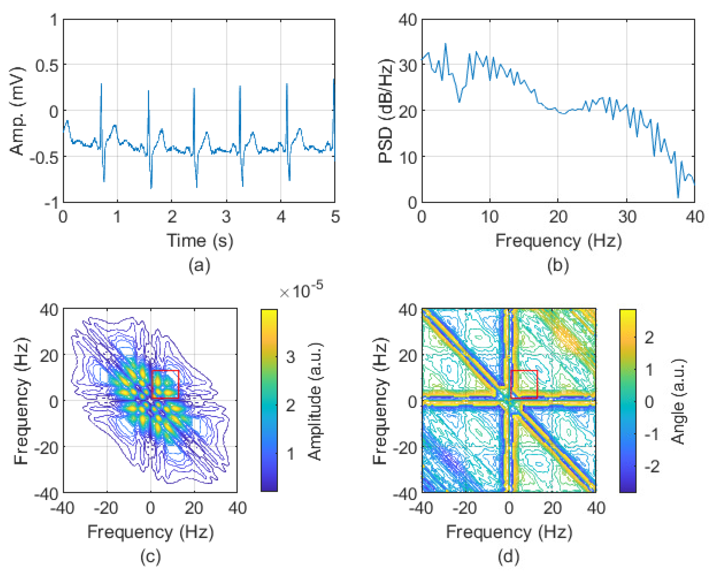
2.1.2. Bispectrum
2.2. AFIB Detection Stage
2.2.1. MIT-BIH Database
2.2.2. Data Preparation
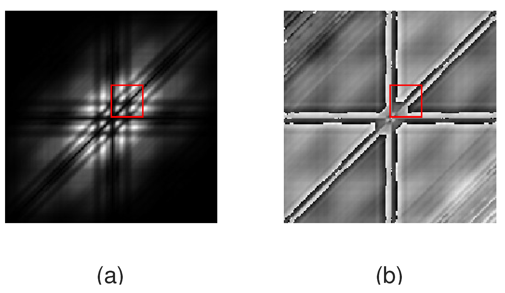
2.2.3. Feature Extraction
2.2.4. Classification
2.3. Statistical Measures Applied for the Classifiers Assessment
3. Results
4. Discussion
4.1. Main Findings of the Study
4.2. Comparison to Other Algorithms
4.3. Strength and Limitations
5. Conclusions
Author Contributions
Funding
Institutional Review Board Statement
Informed Consent Statement
Data Availability Statement
Conflicts of Interest
Abbreviations
| AFIB | Atrial Fibrillation |
| ECG | Electrocardiography/Electrocardiogram |
| CNN | Convolution Neural Network |
| AFIB-NET | CNN for AFIB Detection |
| AFDB | MIT-BIH Atrial Fibrillation Database |
| ROC | Receiver Operating Characteristic |
| AI | Artificial Intelligence |
| HOSA | Higher-Order Statistics Analysis |
| DL | Deep Learning |
| DNN | Deep Neural Network |
| RNN | Recurrent Neural Network |
| LSTM | Long Short-Term Memory Network |
| CNN + LSTM | Hybrid (CNN+LSTM) Network |
| HOS | Higher-Order Statistics |
| SRN | Signal-To-Noise Ratio |
| EEG | Electroencephalogram |
| EMG | Electromyogram |
| GNN | GoogLeNet Network |
| AFL | Atrial Flutter |
| J | Nodal (Junctional) Rhythm |
| FFT | Fast Fourier Transform |
| MBS | MiniBatch Size |
| ILR | Initial Learning Rate |
| TPR | True Positive Rate (Sensitivity, Recall) |
| TNR | True Negative Rate (Specificity) |
| PPV | Precision of Positive Predictive Value |
| NPV | Precision of Negative Predictive Value |
| PV | Prevalence |
| ACC | Accuracy |
| LR+ | Likelihood Ratio of Positive Value |
| LR- | Likelihood Ratio of Negative Value |
| AUC | Area Under Receiver Operating Characteristic (ROC) |
| TP | True Positive |
| FN | False Negative |
| FP | False Positive |
| TN | True Negative |
References
- Kornej, J.; Börschel, C.S.; Benjamin, E.J.; Schnabel, R.B. Epidemiology of Atrial Fibrillation in the 21st Century. Circ. Res. 2020, 127, 4–20. [Google Scholar] [CrossRef]
- Hindricks, G.; Potpara, T.; Dagres, N.; Arbelo, E.; Bax, J.J.; Blomström-Lundqvist, C.; Boriani, G.; Castella, M.; Dan, G.A.; Dilaveris, P.E.; et al. 2020 ESC Guidelines for the diagnosis and management of atrial fibrillation developed in collaboration with the European Association for Cardio-Thoracic Surgery (EACTS): The Task Force for the diagnosis and management of atrial fibrillation of the European Society of Cardiology (ESC) Developed with the special contribution of the European Heart Rhythm Association (EHRA) of the ESC. Eur. Heart J. 2020, 42, 373–498. [Google Scholar] [CrossRef]
- Miyasaka, Y.; Barnes, M.E.; Gersh, B.J.; Cha, S.S.; Bailey, K.R.; Abhayaratna, W.P.; Seward, J.B.; Tsang, T.S. Secular Trends in Incidence of Atrial Fibrillation in Olmsted County, Minnesota, 1980 to 2000, and Implications on the Projections for Future Prevalence. Circulation 2006, 114, 119–125. [Google Scholar] [CrossRef]
- Krijthe, B.P.; Kunst, A.; Benjamin, E.J.; Lip, G.Y.H.; Franco, O.H.; Hofman, A.; Witteman, J.C.M.; Stricker, B.H.; Heeringa, J. Projections on the number of individuals with atrial fibrillation in the European Union, from 2000 to 2060. Eur. Heart J. 2013, 34, 2746–2751. [Google Scholar] [CrossRef]
- Cheniti, G.; Vlachos, K.; Pambrun, T.; Hooks, D.; Frontera, A.; Takigawa, M.; Bourier, F.; Kitamura, T.; Lam, A.; Martin, C.; et al. Atrial Fibrillation Mechanisms and Implications for Catheter Ablation. Front. Physiol. 2018, 9, 1458. [Google Scholar] [CrossRef]
- Veenhuyzen, G.D. Atrial fibrillation. Can. Med. Assoc. J. 2004, 171, 755–760. [Google Scholar] [CrossRef]
- Iwasaki, Y.K.; Nishida, K.; Kato, T.; Nattel, S. Atrial Fibrillation Pathophysiology. Circulation 2011, 124, 2264–2274. [Google Scholar] [CrossRef]
- Jekova, I.; Christov, I.; Krasteva, V. Atrioventricular Synchronization for Detection of Atrial Fibrillation and Flutter in One to Twelve ECG Leads Using a Dense Neural Network Classifier. Sensors 2022, 22, 6071. [Google Scholar] [CrossRef]
- Steinberg, J.S.; O’Connell, H.; Li, S.; Ziegler, P.D. Thirty-Second Gold Standard Definition of Atrial Fibrillation and Its Relationship With Subsequent Arrhythmia Patterns. Circ. Arrhythmia Electrophysiol. 2018, 11, 522. [Google Scholar] [CrossRef]
- Odutayo, A.; Wong, C.X.; Hsiao, A.J.; Hopewell, S.; Altman, D.G.; Emdin, C.A. Atrial fibrillation and risks of cardiovascular disease, renal disease, and death: Systematic review and meta-analysis. BMJ 2016, 354, i4482. [Google Scholar] [CrossRef]
- Wathen, J.E.; Rewers, A.B.; Yetman, A.T.; Schaffer, M.S. Accuracy of ECG interpretation in the pediatric emergency department. Ann. Emerg. Med. 2005, 46, 507–511. [Google Scholar] [CrossRef] [PubMed]
- Raghunath, S.; Pfeifer, J.M.; Ulloa-Cerna, A.E.; Nemani, A.; Carbonati, T.; Jing, L.; vanMaanen, D.P.; Hartzel, D.N.; Ruhl, J.A.; Lagerman, B.F.; et al. Deep Neural Networks Can Predict New-Onset Atrial Fibrillation From the 12-Lead ECG and Help Identify Those at Risk of Atrial Fibrillation–Related Stroke. Circulation 2021, 143, 1287–1298. [Google Scholar] [CrossRef] [PubMed]
- Ghosh, S.K.; Tripathy, R.K.; Paternina, M.R.A.; Arrieta, J.J.; Zamora-Mendez, A.; Naik, G.R. Detection of Atrial Fibrillation from Single Lead ECG Signal Using Multirate Cosine Filter Bank and Deep Neural Network. J. Med. Syst. 2020, 44, 2370. [Google Scholar] [CrossRef] [PubMed]
- Xia, Y.; Wulan, N.; Wang, K.; Zhang, H. Detecting atrial fibrillation by deep convolutional neural networks. Comput. Biol. Med. 2018, 93, 84–92. [Google Scholar] [CrossRef] [PubMed]
- Nurmaini, S.; Tondas, A.E.; Darmawahyuni, A.; Rachmatullah, M.N.; Partan, R.U.; Firdaus, F.; Tutuko, B.; Pratiwi, F.; Juliano, A.H.; Khoirani, R. Robust detection of atrial fibrillation from short-term electrocardiogram using convolutional neural networks. Future Gener. Comput. Syst. 2020, 113, 304–317. [Google Scholar] [CrossRef]
- Sun, Y.; Shen, J.; Jiang, Y.; Huang, Z.; Hao, M.; Zhang, X. MMA-RNN: A multi-level multi-task attention-based recurrent neural network for discrimination and localization of atrial fibrillation. Biomed. Signal Process. Control 2024, 89, 105747. [Google Scholar] [CrossRef]
- Sujadevi, V.G.; Soman, K.P.; Vinayakumar, R. Real-Time Detection of Atrial Fibrillation from Short Time Single Lead ECG Traces Using Recurrent Neural Networks. In Intelligent Systems Technologies and Applications, Proceedings of the Third International Symposium on Intelligent Systems Technologies and Applications (ISTA’17), Manipal, India, 13–16 September 2017; Thampi, S.M., Mitra, S., Mukhopadhyay, J., Li, K.C., James, A.P., Berretti, S., Eds.; Springer: Cham, Switzerland, 2018; pp. 212–221. [Google Scholar]
- Gündüz, A.F.; Talu, M.F. Atrial fibrillation classification and detection from ECG recordings. Biomed. Signal Process. Control 2023, 82, 104531. [Google Scholar] [CrossRef]
- Faust, O.; Shenfield, A.; Kareem, M.; San, T.R.; Fujita, H.; Acharya, U.R. Automated detection of atrial fibrillation using long short-term memory network with RR interval signals. Comput. Biol. Med. 2018, 102, 327–335. [Google Scholar] [CrossRef] [PubMed]
- Murat, F.; Sadak, F.; Yildirim, O.; Talo, M.; Murat, E.; Karabatak, M.; Demir, Y.; Tan, R.S.; Acharya, U.R. Review of Deep Learning-Based Atrial Fibrillation Detection Studies. Int. J. Environ. Res. Public Health 2021, 18, 11302. [Google Scholar] [CrossRef]
- Iftene, A.; Burlacu, A.; Gifu, D. Atrial Fibrillation Detection Based on Deep Learning Models. Procedia Comput. Sci. 2022, 207, 3752–3760. [Google Scholar] [CrossRef]
- Subramanyan, L.; Ganesan, U. A novel deep neural network for detection of Atrial Fibrillation using ECG signals. Knowl.-Based Syst. 2022, 258, 109926. [Google Scholar] [CrossRef]
- Petmezas, G.; Haris, K.; Stefanopoulos, L.; Kilintzis, V.; Tzavelis, A.; Rogers, J.A.; Katsaggelos, A.K.; Maglaveras, N. Automated Atrial Fibrillation Detection using a Hybrid CNN-LSTM Network on Imbalanced ECG Datasets. Biomed. Signal Process. Control 2021, 63, 102194. [Google Scholar] [CrossRef]
- Ebrahimi, Z.; Loni, M.; Daneshtalab, M.; Gharehbaghi, A. A review on deep learning methods for ECG arrhythmia classification. Expert Syst. Appl. X 2020, 7, 100033. [Google Scholar] [CrossRef]
- Ansari, Y.; Mourad, O.; Qaraqe, K.; Serpedin, E. Deep learning for ECG Arrhythmia detection and classification: An overview of progress for period 2017–2023. Front. Physiol. 2023, 14, 1246746. [Google Scholar] [CrossRef]
- Chua, K.C.; Chandran, V.; Acharya, U.R.; Lim, C.M. Application of higher order statistics/spectra in biomedical signals—A review. Med. Eng. Phys. 2010, 32, 679–689. [Google Scholar] [CrossRef]
- Nikias, C.; Mendel, J. Signal processing with higher-order spectra. IEEE Signal Process. Mag. 1993, 10, 10–37. [Google Scholar] [CrossRef]
- Mendel, J. Tutorial on higher-order statistics (spectra) in signal processing and system theory: Theoretical results and some applications. Proc. IEEE 1991, 79, 278–305. [Google Scholar] [CrossRef]
- Sigl, J.C.; Chamoun, N.G. An introduction to bispectral analysis for the electroencephalogram. J. Clin. Monit. 1994, 10, 392–404. [Google Scholar] [CrossRef]
- Khoshnevis, S.A.; Sankar, R. Applications of Higher Order Statistics in Electroencephalography Signal Processing: A Comprehensive Survey. IEEE Rev. Biomed. Eng. 2020, 13, 169–183. [Google Scholar] [CrossRef]
- Mahmoodian, N.; Haddadnia, J.; Illanes, A.; Boese, A.; Friebe, M. Seizure prediction with cross-higher-order spectral analysis of EEG signals. Signal Image Video Process. 2020, 14, 821–828. [Google Scholar] [CrossRef]
- Sezgin, N. Analysis of EMG Signals in Aggressive and Normal Activities by Using Higher-Order Spectra. Sci. World J. 2012, 2012, 478952. [Google Scholar] [CrossRef]
- Kotriwar, Y.; Kachhara, S.; Harikrishnan, K.P.; Ambika, G. Higher order spectral analysis of ECG signals. arXiv 2018, arXiv:1809.08451. [Google Scholar]
- Martis, R.J.; Acharya, U.R.; Prasad, H.; Chua, C.K.; Lim, C.M.; Suri, J.S. Application of higher order statistics for atrial arrhythmia classification. Biomed. Signal Process. Control 2013, 8, 888–900. [Google Scholar] [CrossRef]
- Liu, S.; Shao, J.; Kong, T.; Malekian, R. ECG Arrhythmia Classification using High Order Spectrum and 2D Graph Fourier Transform. Appl. Sci. 2020, 10, 4741. [Google Scholar] [CrossRef]
- Deka, B.; Deka, D. Nonlinear analysis of heart rate variability signals in meditative state: A review and perspective. Biomed. Eng. Online 2023, 22, 35. [Google Scholar] [CrossRef]
- Xu, J.; Ye, P.; Li, Q.; Du, H.; Liu, Y.; Doermann, D. Blind Image Quality Assessment Based on High Order Statistics Aggregation. IEEE Trans. Image Process. 2016, 25, 4444–4457. [Google Scholar] [CrossRef]
- Sanaullah, M. A Review of Higher Order Statistics and Spectra in Communication Systems. Glob. J. Sci. Front. Res. 2013, 31–50. [Google Scholar] [CrossRef]
- Ould-Baba, H.; Robin, V.; Antoni, J. Concise formulae for the cumulant matrices of a random vector. Linear Algebra Its Appl. 2015, 485, 392–416. [Google Scholar] [CrossRef]
- La Rosa, J.J.G.d.; Agüera-Pérez, A.; Palomares-Salas, J.C.; Moreno-Muñoz, A. Higher-order statistics: Discussion and interpretation. Measurement 2013, 46, 2816–2827. [Google Scholar] [CrossRef]
- Szegedy, C.; Liu, W.; Jia, Y.; Sermanet, P.; Reed, S.; Anguelov, D.; Erhan, D.; Vanhoucke, V.; Rabinovich, A. Going Deeper with Convolutions. arXiv 2014, arXiv:1409.4842. [Google Scholar] [CrossRef]
- Goldberger, A.L.; Amaral, L.A.N.; Glass, L.; Hausdorff, J.M.; Ivanov, P.C.; Mark, R.G.; Mietus, J.E.; Moody, G.B.; Peng, C.K.; Stanley, H.E. PhysioBank, PhysioToolkit, and PhysioNet: Components of a New Research Resource for Complex Physiologic Signals. Circulation 2000, 101, e215–e220. [Google Scholar] [CrossRef] [PubMed]
- Swami, A. HOSA—Higher Order Spectral Analysis Toolbox. MATLAB Central File Exchange. 2023. Available online: https://www.mathworks.com/matlabcentral/fileexchange/3013-hosa-higher-order-spectral-analysis-toolbox (accessed on 19 December 2023).
- Alcaraz, R.; Rieta, J.J. Surface ECG organization analysis to predict paroxysmal atrial fibrillation termination. Comput. Biol. Med. 2009, 39, 697–706. [Google Scholar] [CrossRef]
- Castells, F.; Rieta, J.J.; Millet, J.; Zarzoso, V. Spatiotemporal Blind Source Separation Approach to Atrial Activity Estimation in Atrial Tachyarrhythmias. IEEE Trans. Biomed. Eng. 2005, 52, 258–267. [Google Scholar] [CrossRef]
- Diaz, J.; Escalona, O.; Castro, N.; Anderson, J.; Glover, B.; Manoharan, G. Predicting transthoracic defibrillation shocks outcome in the cardioversion of atrial fibrillation employing support vector machines. In Proceedings of the 2010 Computing in Cardiology, Belfast, UK, 26–29 September 2010; pp. 741–744. [Google Scholar]
- Llinares, R.; Igual, J. Exploiting periodicity to extract the atrial activity in atrial arrhythmias. EURASIP J. Adv. Signal Process. 2011, 2011, 1176. [Google Scholar] [CrossRef]
- Petrutiu, S.; Ng, J.; Nijm, G.M.; Al-Angari, H.; Swiryn, S.; Sahakian, A.V. Atrial fibrillation and waveform characterization. IEEE Eng. Med. Biol. Mag. 2006, 25, 24–30. [Google Scholar] [CrossRef]
- Stridh, M.; Sornmo, L.; Meurling, C.J.; Olsson, S.B. Sequential Characterization of Atrial Tachyarrhythmias Based on ECG Time-Frequency Analysis. IEEE Trans. Biomed. Eng. 2004, 51, 100–114. [Google Scholar] [CrossRef]
- Stridh, M.; Bollmann, A.; Olsson, S.B.; Sornmo, L. Detection and feature extraction of atrial tachyarrhythmias. IEEE Eng. Med. Biol. Mag. 2006, 25, 31–39. [Google Scholar] [CrossRef]
- Hayes, M.H. Statistical Digital Signal Processing and Modeling, 1st ed.; John Wiley & Sons, Inc.: Hoboken, NJ, USA, 1996. [Google Scholar]
- Stoica, P.; Moses, R.L. Spectral Analysis of Signals/Petre Stoica and Randolph Moses; Pearson/Prentice Hall: Upper Saddle River, NJ, USA, 2005. [Google Scholar]
- Grimes, D.A.; Schulz, K.F. Refining clinical diagnosis with likelihood ratios. Lancet 2005, 365, 1500–1505. [Google Scholar] [CrossRef]
- Peng, P.; Coyle, A.; Newgard, C.D. Likelihood Ratios for the Emergency Physician. Acad. Emerg. Med. 2018, 25, 958–965. [Google Scholar] [CrossRef]
- Junge, M.R.J.; Dettori, J.R. ROC Solid: Receiver Operator Characteristic (ROC) Curves as a Foundation for Better Diagnostic Tests. Glob. Spine J. 2017, 8, 424–429. [Google Scholar] [CrossRef]
- Osowski, S.; Hoai, L.T.; Markiewicz, T. Support Vector Machine-Based Expert System for Reliable Heartbeat Recognition. IEEE Trans. Biomed. Eng. 2004, 51, 582–589. [Google Scholar] [CrossRef]
- Mousavi, S.; Afghah, F.; Razi, A.; Acharya, U.R. ECGNET: Learning Where to Attend for Detection of Atrial Fibrillation with Deep Visual Attention. In Proceedings of the 2019 IEEE EMBS International Conference on Biomedical & Health Informatics (BHI), Chicago, IL, USA, 19–22 May 2019; pp. 1–4. [Google Scholar] [CrossRef]
- Radhakrishnan, T.; Karhade, J.; Ghosh, S.; Muduli, P.; Tripathy, R.; Acharya, U.R. AFCNNet: Automated detection of AF using chirplet transform and deep convolutional bidirectional long short term memory network with ECG signals. Comput. Biol. Med. 2021, 137, 104783. [Google Scholar] [CrossRef]
- Yang, W.; Wang, D.; Fan, W.; Zhang, G.; Li, C.; Liu, T. Automated atrial fibrillation and ventricular fibrillation recognition using a multi-angle dual-channel fusion network. Artif. Intell. Med. 2023, 145, 102680. [Google Scholar] [CrossRef]
- Marsanova, L.; Nemcova, A.; Smisek, R.; Vitek, M.; Smital, L. Single-Feature Method for Fast Atrial Fibrillation Detection in ECG Signals. In Proceedings of the 2020 Computing in Cardiology, Rimini, Italy, 13–16 September 2020; pp. 1–4. [Google Scholar] [CrossRef]
- Wang, J.; Wang, P.; Wang, S. Automated detection of atrial fibrillation in ECG signals based on wavelet packet transform and correlation function of random process. Biomed. Signal Process. Control 2020, 55, 101662. [Google Scholar] [CrossRef]
- Kumar, M.; Pachori, R.B.; Rajendra Acharya, U. Automated diagnosis of atrial fibrillation ECG signals using entropy features extracted from flexible analytic wavelet transform. Biocybern. Biomed. Eng. 2018, 38, 564–573. [Google Scholar] [CrossRef]
- Tripathy, R.K.; Paternina, M.R.A.; Arrieta, J.G.; Pattanaik, P. Automated Detection Of Atrial Fibrillation Ecg Signals Using Two Stage Vmd And Atrial Fibrillation Diagnosis Index. J. Mech. Med. Biol. 2017, 17, 1740044. [Google Scholar] [CrossRef]
- Asgari, S.; Mehrnia, A.; Moussavi, M. Automatic detection of atrial fibrillation using stationary wavelet transform and support vector machine. Comput. Biol. Med. 2015, 60, 132–142. [Google Scholar] [CrossRef]
- Lee, J.; Reyes, B.A.; McManus, D.D.; Maitas, O.; Chon, K.H. Atrial Fibrillation Detection Using an iPhone 4S. IEEE Trans. Biomed. Eng. 2013, 60, 203–206. [Google Scholar] [CrossRef]
- Huang, C.; Ye, S.; Chen, H.; Li, D.; He, F.; Tu, Y. A Novel Method for Detection of the Transition Between Atrial Fibrillation and Sinus Rhythm. IEEE Trans. Biomed. Eng. 2011, 58, 1113–1119. [Google Scholar] [CrossRef]
- Tateno, K.; Glass, L. Automatic detection of atrial fibrillation using the coefficient of variation and density histograms of RR and dRR intervals. Med. Biol. Eng. Comput. 2001, 39, 664–671. [Google Scholar] [CrossRef]


| Episode | № | Min | Max | Mean | Total |
|---|---|---|---|---|---|
| [s] | [s] | [s] | [s] | ||
| AFIB | 291 | 1.684 | 36,822.864 | 1155.436 | 336,231.984 |
| AFL | 14 | 3.532 | 3390.912 | 419.794 | 5877.116 |
| Nodal | 12 | 1.524 | 86.016 | 27.582 | 330.980 |
| N (other) | 288 | 4.252 | 30,981.372 | 1739.440 | 500,958.808 |
| Layer | Type | Filter Size | Number of Filters | Stride | Activations | Number of Learnables |
|---|---|---|---|---|---|---|
| 1 | Image Input | - | - | - | 24 × 24 × 1 × 1 | 0 |
| 2 | Convolution | 3 × 3 | 8 | [1 1] | 24 × 24 × 8 × 1 | 80 |
| 3 | Batch Normalization | - | - | - | 24 × 24 × 8 × 1 | 16 |
| 4 | ReLu | - | - | - | 24 × 24 × 8 × 1 | 0 |
| 5 | Max Pooling | - | - | [1 1] | 23 × 23 × 8 × 1 | 0 |
| 6 | Convolution | 3 × 3 | 16 | [1 1] | 23 × 23 × 16 × 1 | 1168 |
| 7 | Batch Normalization | - | - | - | 23 × 23 × 16 × 1 | 32 |
| 8 | ReLu | - | - | - | 23 × 23 × 16 × 1 | 0 |
| 9 | Ma × Pooling | - | - | [1 1] | 22 × 22 × 16 × 1 | 0 |
| 10 | Convolution | 3 × 3 | 32 | [1 1] | 22 × 22 × 32 × 1 | 4640 |
| 11 | Batch Normalization | - | - | - | 22 × 22 × 32 × 1 | 64 |
| 12 | ReLu | - | - | - | 22 × 22 × 32 × 1 | 0 |
| 13 | Max Pooling | - | - | [1 1] | 11 × 11 × 32 × 1 | 0 |
| 14 | Convolution | 3 × 3 | 64 | [2 2] | 11 × 11 × 64 × 1 | 18,496 |
| 15 | Batch Normalization | - | - | - | 11 × 11 × 64 × 1 | 128 |
| 16 | ReLu | - | - | - | 11 × 11 × 64 × 1 | 0 |
| 17 | Max Pooling | - | - | [1 1] | 5 × 5 × 64 × 1 | 0 |
| 18 | Convolution | 3 × 3 | 128 | [2 2] | 5 × 5 × 128 × 1 | 73,856 |
| 19 | Batch Normalization | - | - | - | 5 × 5 × 128 × 1 | 256 |
| 20 | ReLu | - | - | - | 5 × 5 × 128 × 1 | 0 |
| 21 | Fully Connected | - | - | - | 1 × 1 × 2 × 1 | 6402 |
| 22 | Softmax | - | - | - | 1 × 1 × 2 × 1 | 0 |
| 23 | Classification Output | - | - | - | 1 × 1 × 2 × 1 | 0 |
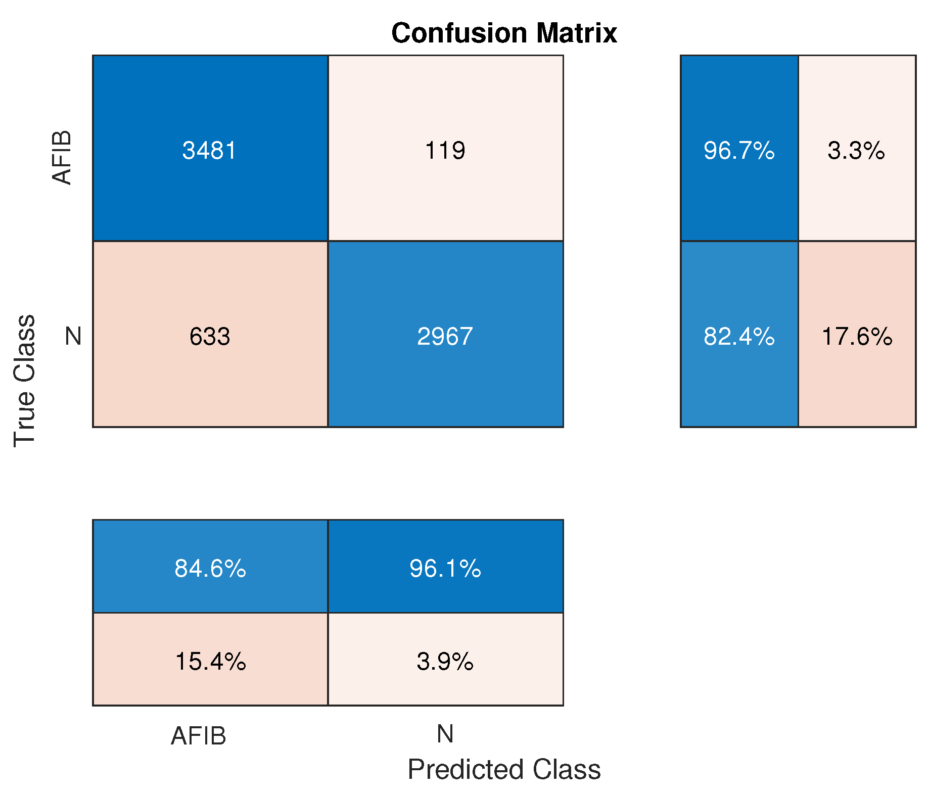
| Measure | AFIB-NET | GooLeNet (GNN) |
|---|---|---|
| Sensitivity (TPR) | 0.953 | 0.967 |
| Specificity (TNR) | 0.937 | 0.824 |
| PPV | 0.938 | 0.846 |
| NPV | 0.952 | 0.961 |
| PV | 0.500 | 0.500 |
| ACC | 0.945 | 0.896 |
| LR+ | 15.127 | 5.494 |
| LR- | 0.050 | 0.040 |
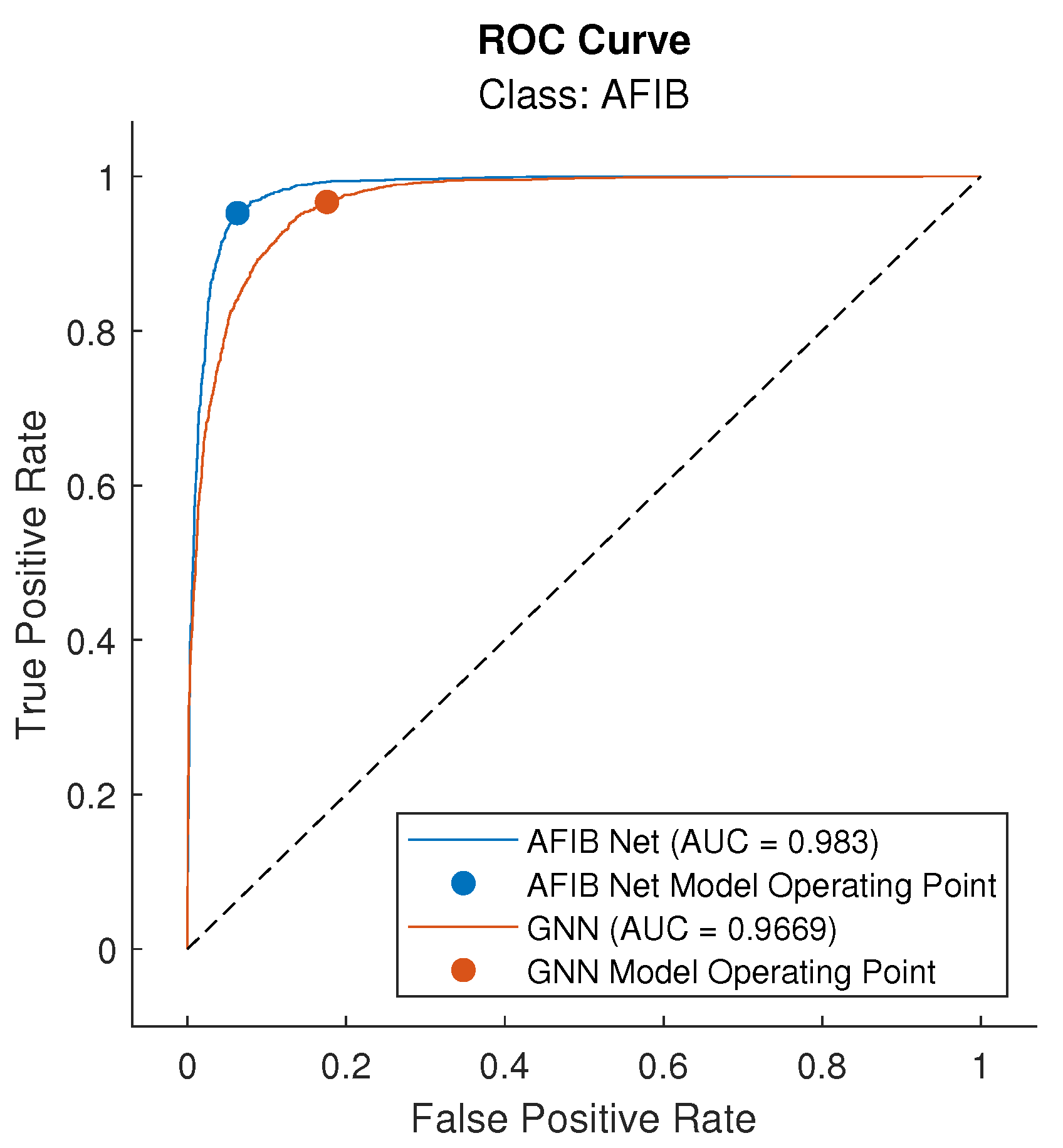
| AUC | 0.983 | 0.967 |
| 0.945 | 0.902 | |
| 0.952 | 0.964 |
| Method Proposed by | Sensitivity (%) | Specificity (%) |
|---|---|---|
| RADHAKRISHNAN et al. (2021) [58] | 99.17 | 98.90 |
| Marsanova et al. (2020) [60] | 96.32 | 98.61 |
| Wang et al. (2020) [61] | 98.70 | 98.90 |
| Mousavi et al. (2019) [57] | 99.53 | 99.26 |
| Xia et al. (2018) (STFT) [14] | 98.34 | 98.24 |
| Xia et al. (2018) (SWT) [14] | 98.79 | 97.87 |
| Kumar et al. (2018) [62] | 95.80 | 97.60 |
| Tripathy et al. (2017) [63] | 97.77 | 98.67 |
| Asgari et al. (2015) [64] | 97.00 | 97.10 |
| Lee et al. (2013) (RMSSD) [65] | 90.49 | 94.17 |
| Lee et al. (2013) (ShE) [65] | 74.15 | 96.81 |
| Lee et al. (2013) (SamE) [65] | 97.26 | 99.61 |
| Huang et al. (2011) [66] | 96.10 | 98.10 |
| Tateno et al. (2001) [67] | 94.40 | 97.20 |
| AFIB (Proposed work) | 95.30 | 96.70 |
| GNN (Proposed work) | 93.70 | 82.00 |
Disclaimer/Publisher’s Note: The statements, opinions and data contained in all publications are solely those of the individual author(s) and contributor(s) and not of MDPI and/or the editor(s). MDPI and/or the editor(s) disclaim responsibility for any injury to people or property resulting from any ideas, methods, instructions or products referred to in the content. |
© 2024 by the authors. Licensee MDPI, Basel, Switzerland. This article is an open access article distributed under the terms and conditions of the Creative Commons Attribution (CC BY) license (https://creativecommons.org/licenses/by/4.0/).
Share and Cite
Mika, B.; Komorowski, D. Higher-Order Spectral Analysis Combined with a Convolution Neural Network for Atrial Fibrillation Detection-Preliminary Study. Sensors 2024, 24, 4171. https://doi.org/10.3390/s24134171
Mika B, Komorowski D. Higher-Order Spectral Analysis Combined with a Convolution Neural Network for Atrial Fibrillation Detection-Preliminary Study. Sensors. 2024; 24(13):4171. https://doi.org/10.3390/s24134171
Chicago/Turabian StyleMika, Barbara, and Dariusz Komorowski. 2024. "Higher-Order Spectral Analysis Combined with a Convolution Neural Network for Atrial Fibrillation Detection-Preliminary Study" Sensors 24, no. 13: 4171. https://doi.org/10.3390/s24134171