
Cost-Effective Data Acquisition Systems for Advanced Structural Health Monitoring


Abstract
1. Introduction
2. Device Fabrication and Features
3. Description of Data Storage and Processing
4. Validation Tests and Case Study
4.1. Offset Test
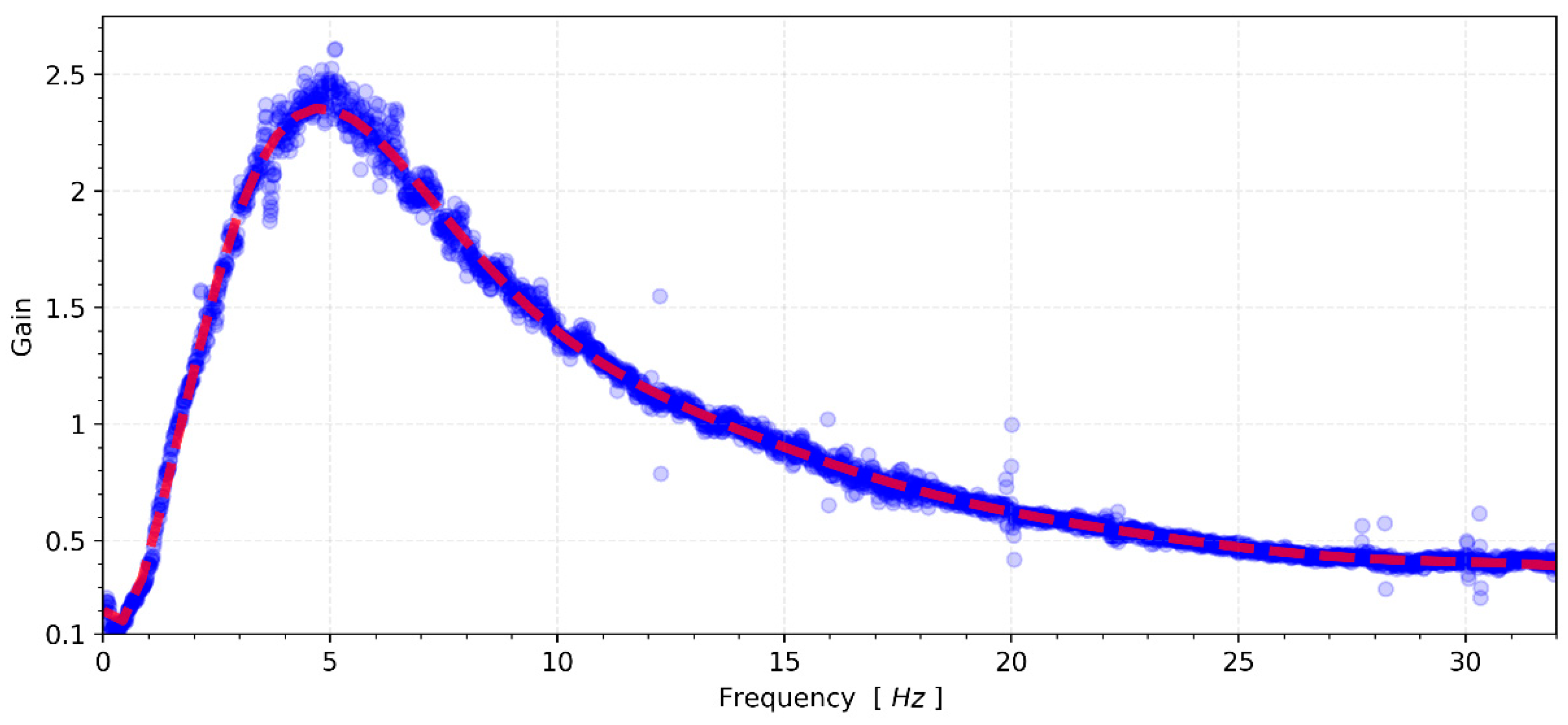
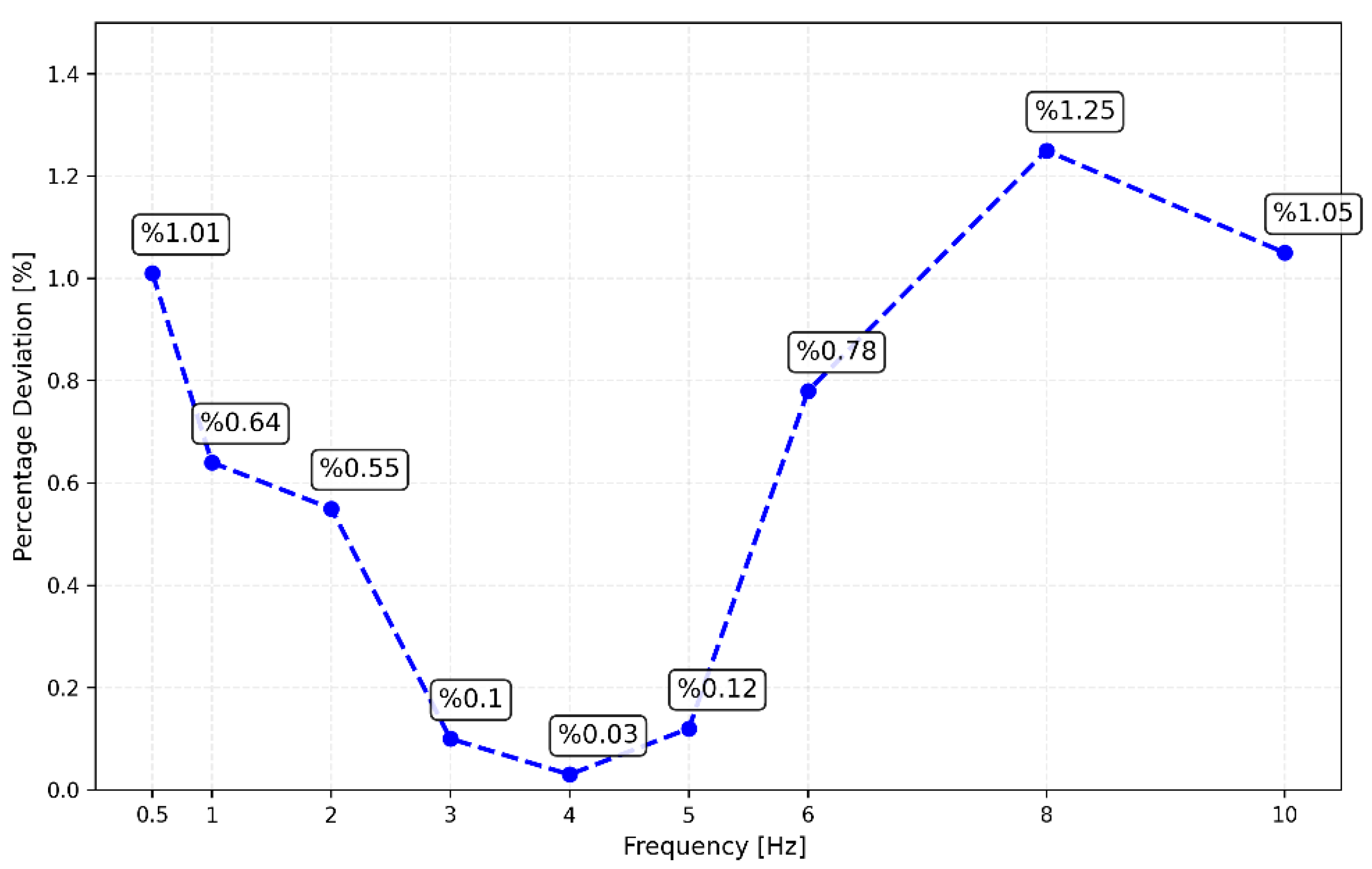
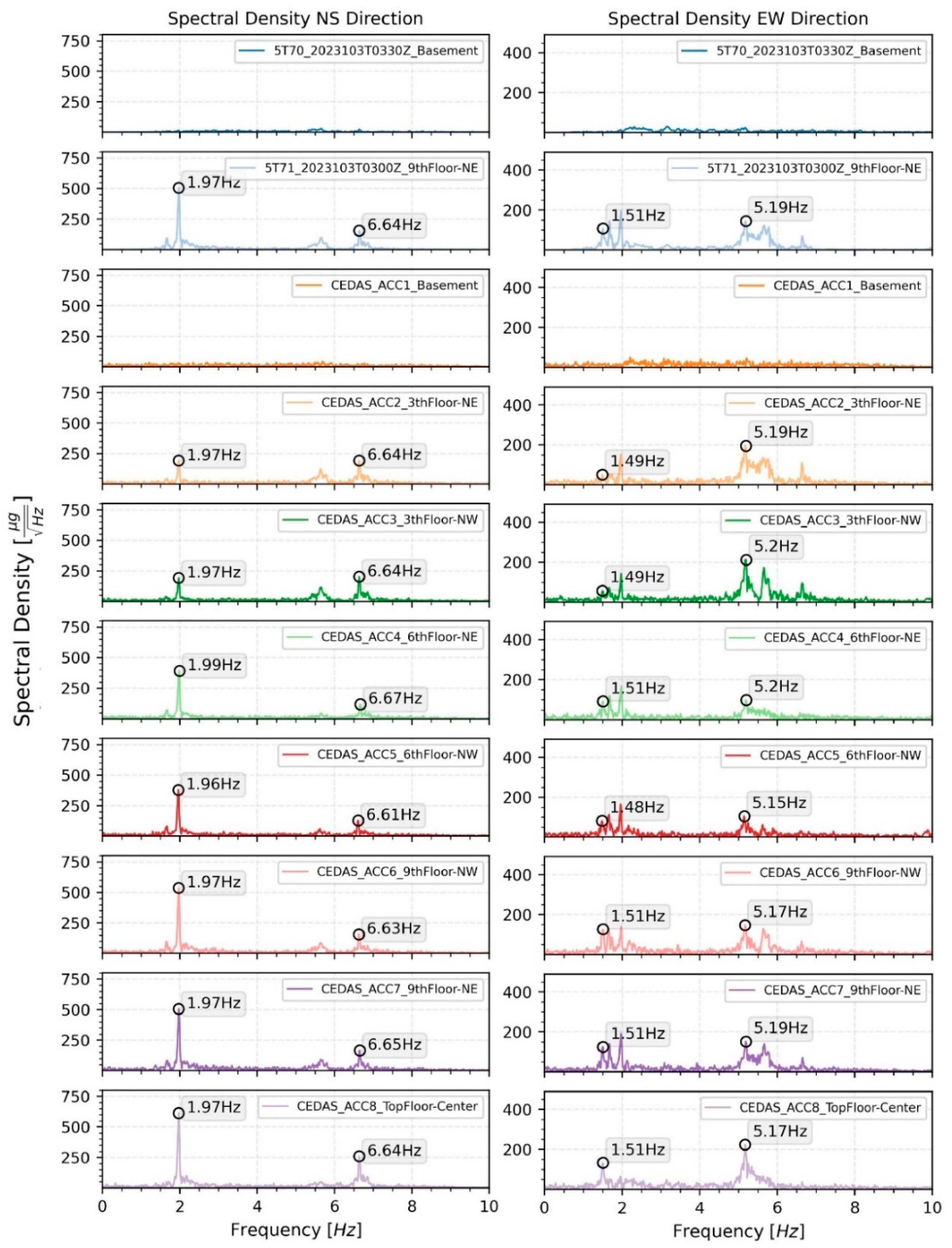
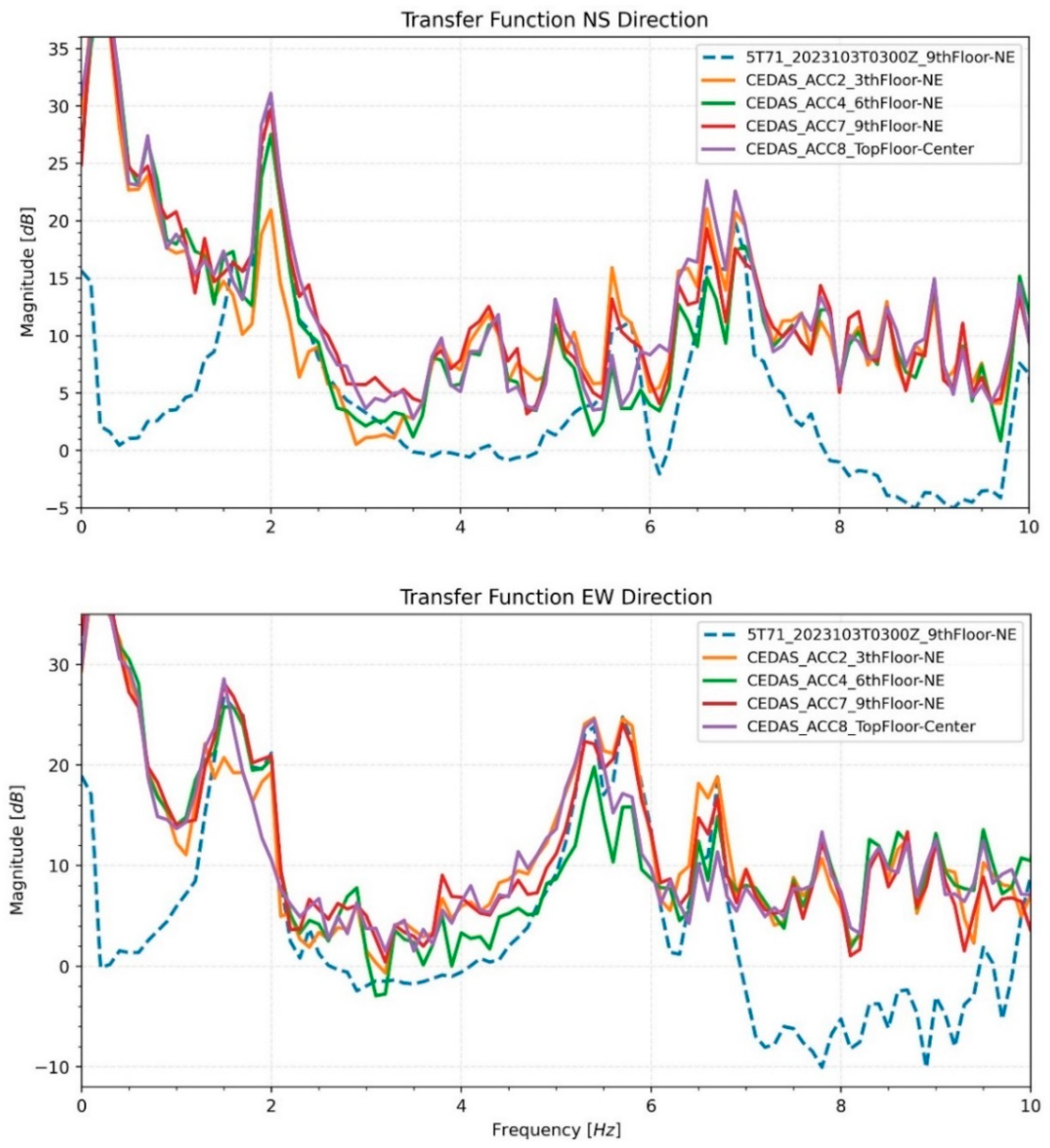
4.2. Frequency Response Tests
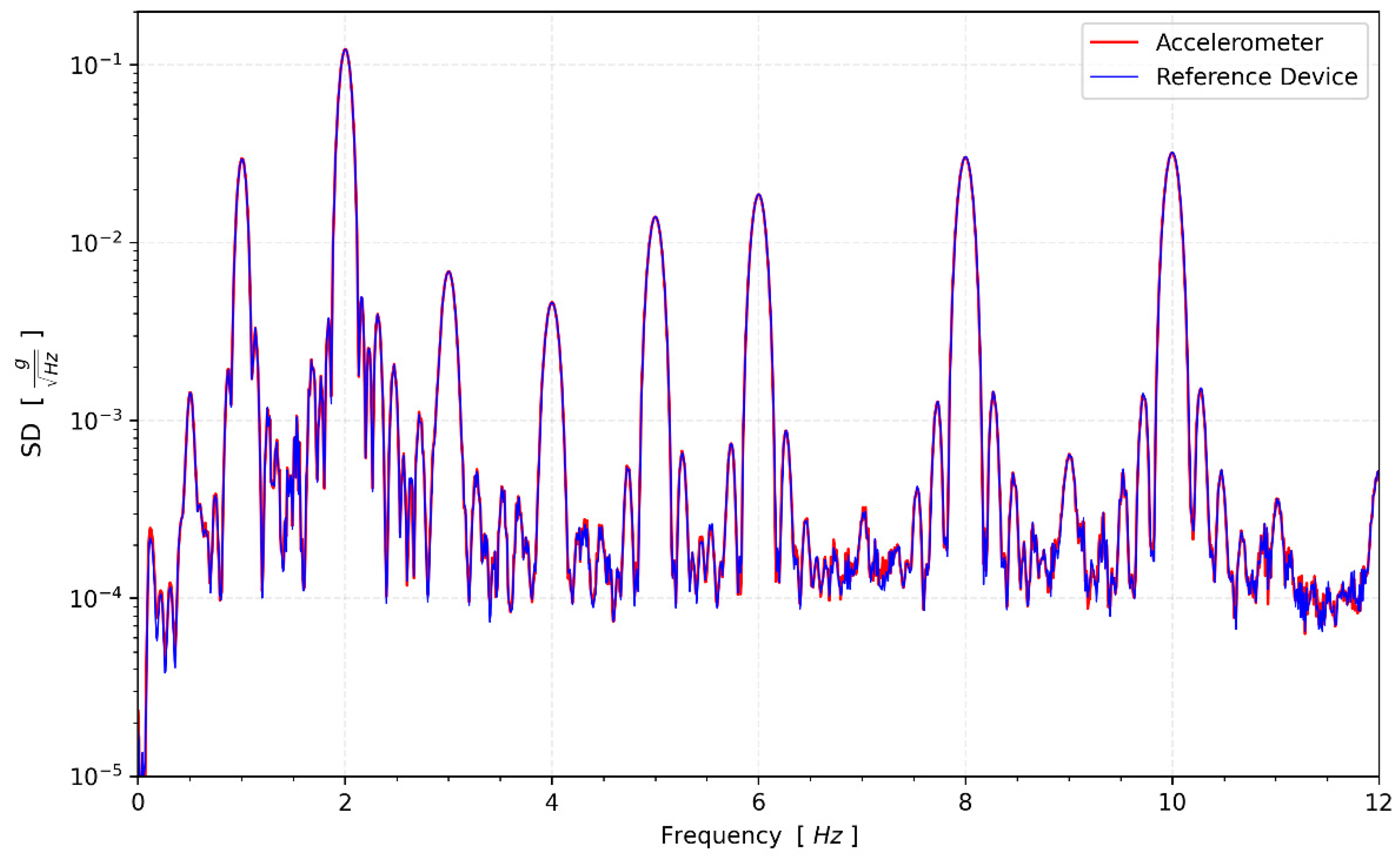
4.3. Noise Test
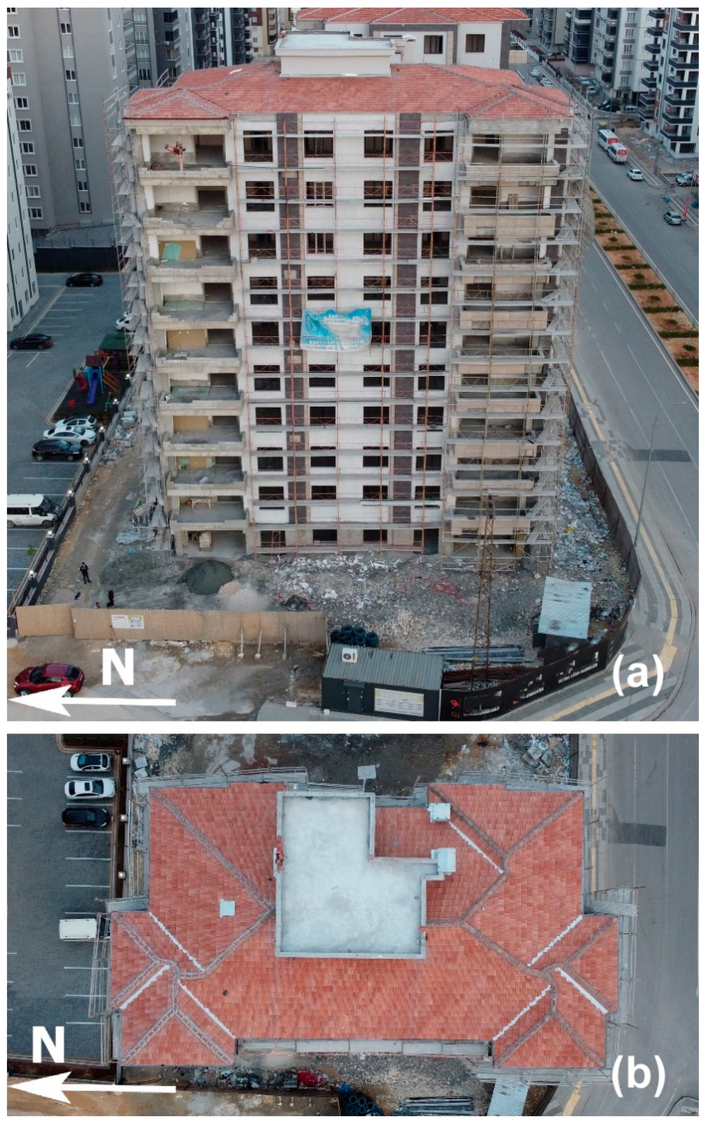
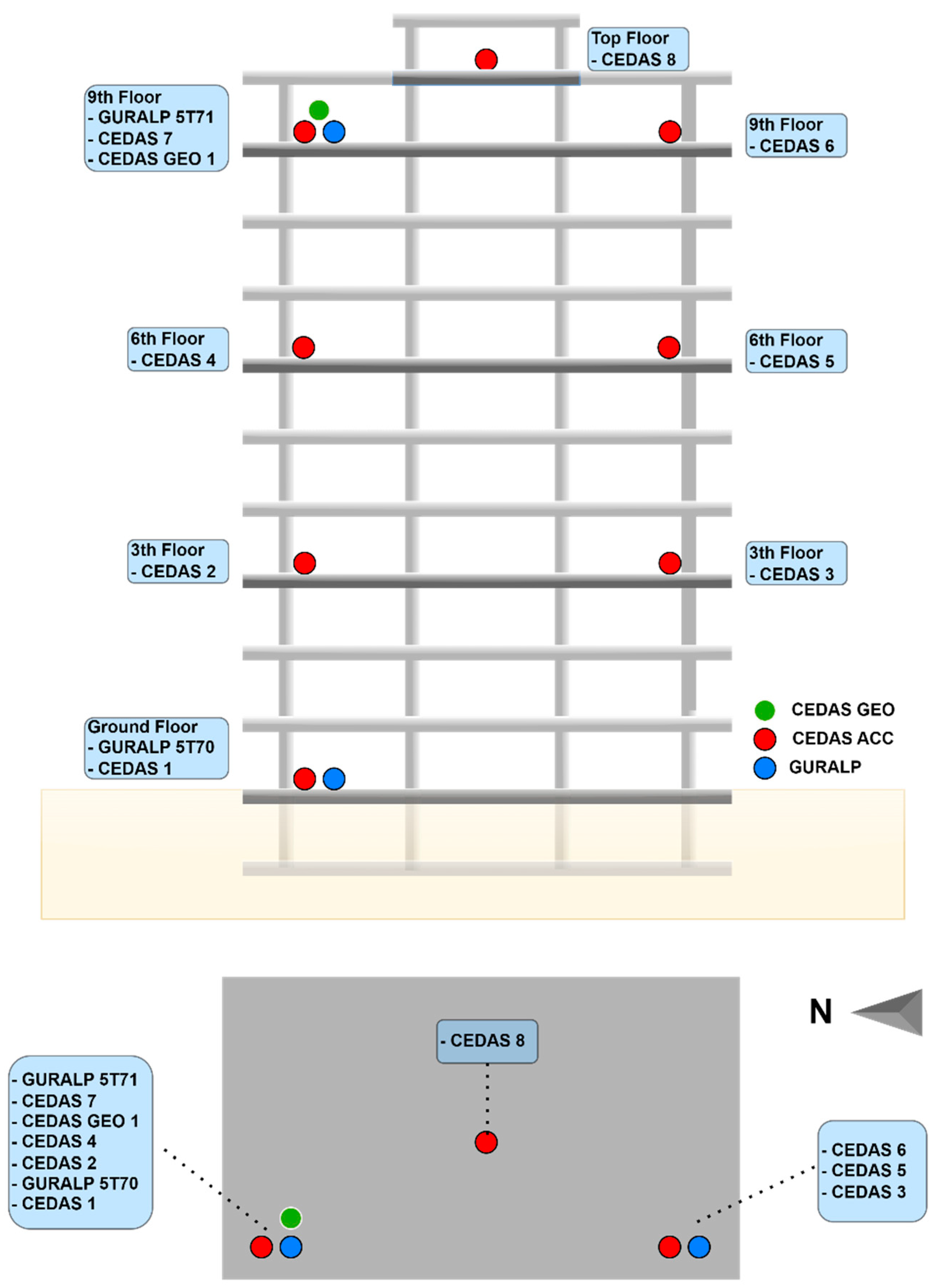
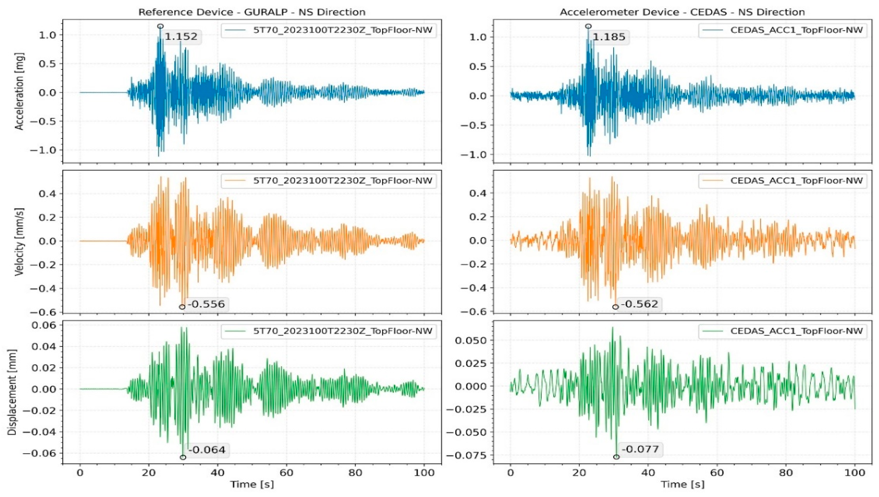
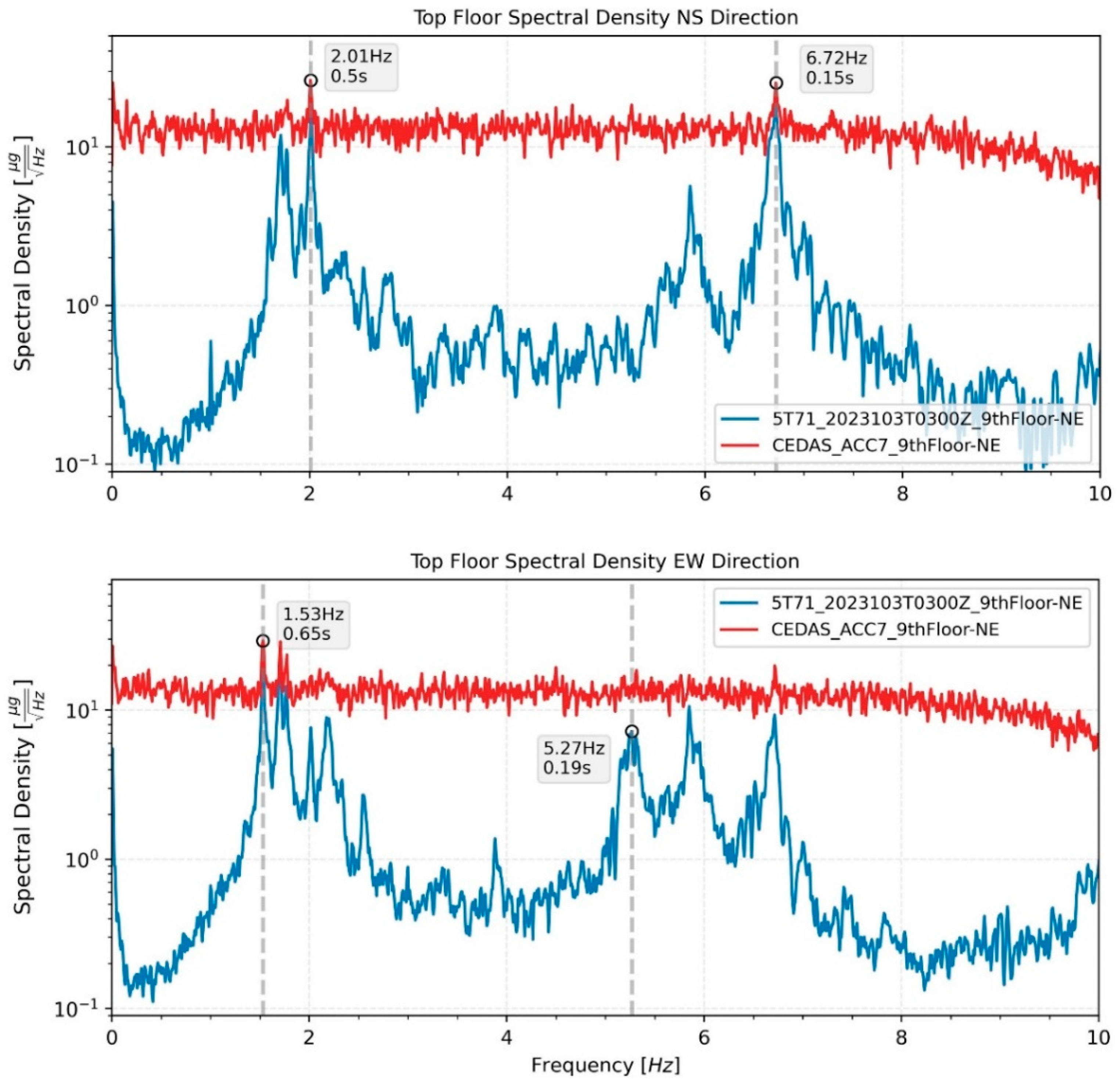
4.4. Field Test
5. Conclusions and Future Studies
Author Contributions
Funding
Institutional Review Board Statement
Informed Consent Statement
Data Availability Statement
Acknowledgments
Conflicts of Interest
References
- Eddy, D.S.; Sparks, D.R. Application of MEMS technology in automotive sensors and actuators. Proc. IEEE 1998, 86, 1747–1755. [Google Scholar] [CrossRef]
- Tang, W.C. MEMS applications in space exploration. In Proceedings of the Micromachined Devices and Components III, Austin, TX, USA, 29–30 September 1997; Volume 3224, pp. 202–212. [Google Scholar] [CrossRef]
- D’Alessandro, A.; Scudero, S.; Vitale, G. A Review of the Capacitive MEMS for Seismology. Sensors 2019, 19, 3093. [Google Scholar] [CrossRef] [PubMed]
- Roylance, L.M.; Angell, J.B. A batch-fabricated silicon accelerometer. IEEE Trans. Electron Devices 1979, 26, 1911–1917. [Google Scholar] [CrossRef]
- Crognale, M.; Rinaldi, C.; Potenza, F.; Gattulli, V.; Colarieti, A.; Franchi, F. Developing and Testing High-Performance SHM Sensors Mounting Low-Noise MEMS Accelerometers. Sensors 2024, 24, 2435. [Google Scholar] [CrossRef] [PubMed]
- López-Castro, B.; Haro-Baez, A.G.; Arcos-Aviles, D.; Barreno-Riera, M.; Landázuri-Avilés, B. A Systematic Review of Structural Health Monitoring Systems to Strengthen Post-Earthquake Assessment Procedures. Sensors 2022, 22, 9206. [Google Scholar] [CrossRef] [PubMed]
- ANSS Working Group on Instrumentation, Siting, Installation, and Site Metadata of the Advanced National Seismic System Technical Integration Committee. Instrumentation Guidelines for the Advanced National Seismic System; U.S. Geological Survey: Reston, VA, USA, 2008; Open-File Report 2008-1262. [Google Scholar]
- ANSS Technical Integration Committee (TIC). Technical Guidelines for the Implementation of the Advanced National Seismic System; U.S. Geological Survey: Reston, VA, USA, 2002; Open-File Report 2002-9296. [Google Scholar]
- Hutt, C.R.; Evans, J.R.; Followill, F.; Nigbor, R.L.; Wielandt, E. Guidelines for Standardized Testing of Broadband Seismometers and Accelerometers; U.S. Geological Survey: Reston, VA, USA, 2010; Open-File Report 2009-1295; p. 62. [Google Scholar]
- D’Alessando, A.; D’Anna, G. Suitability of Low-Cost Three-Axis MEMS Accelerometers in Strong-Motion Seismology: Tests on the LIS331DLH (iPhone) Accelerometer. Bull. Seismol. Soc. Am. 2013, 103, 2906–2913. [Google Scholar] [CrossRef]
- Clayton, R.; Heaton, T.; Chandy, K.; Krause, A.; Kohler, M.; Bunn, J.; Guy, R.; Olson, M.; Faulkner, M.; Cheng, M.; et al. Community Seismic Network. Ann. Geophys. 2011, 54, 738–747. [Google Scholar] [CrossRef]
- Cochran, E.S.; Lawrence, J.F.; Christensen, C.; Jakka, R. The Quake-Catcher Network: Citizen science expanding seismic horizons. Seismol. Res. Lett. 2009, 80, 26–30. [Google Scholar] [CrossRef]
- D’Alessandro, A.; Luzio, D.; D’Anna, G. Urban MEMS based seismic network for post-earthquakes rapid disaster assessment. Adv. Geosci. 2014, 40, 1–9. [Google Scholar] [CrossRef]
- Fleming, K.; Picozzi, M.; Milkereit, C.; Kuhnlenz, F.; Lichtblau, B.; Fischer, J.; Zulfikar, C.; Ozel, O. The Self-organizing Seismic Early Warning Information Network (SOSEWIN). Seismol. Res. Lett. 2009, 80, 755–771. [Google Scholar] [CrossRef]
- Kohler, M.D.; Hao, S.; Mishra, N.; Govindan, R.; Nigbor, R. ShakeNet A Portable Wireless Sensor Network for Instrumenting Large Civil Structures; U.S. Geological Survey: Reston, VA, USA, 2015; Open-File Report 2015-1134; p. 31. [Google Scholar] [CrossRef]
- Nof, R.; Chung, A.; Meng, L.; Kong, Q.; Richard, A. MEMS Accelerometers Mini Array (MAMA)—A Low Cost Solution For Array Based Earthquake Early Warning System. Earthq. Spectra 2019, 35, 21–38. [Google Scholar] [CrossRef]
- Available online: https://www.phidgets.com/ (accessed on 1 February 2024).
- Available online: http://o-navi.com/ (accessed on 1 February 2024).
- Patrick, W. The history of the accelerometer 1920s-1996—Prologue and Epilogue. Sound Vib. 2007, 41, 84–92. [Google Scholar]
- Evans, J.; Allen, R.; Chung, A.; Cochran, E.; Guy, R.; Hellweg, M.; Lawrence, J. Performance of Several Low-Cost Accelerometers. Seismol. Res. Lett. 2014, 85, 147–158. [Google Scholar] [CrossRef]
- Sabato, A.; Niezrecki, C.; Fortino, G. Wireless MEMS-Based Accelerometer Sensor Boards for Structural Vibration Monitoring: A Review. IEEE Sens. J. 2017, 17, 226–235. [Google Scholar] [CrossRef]
- Ambrož, M. Raspberry Pi as a low-cost data acquisition system for human powered vehicles. Measurement 2017, 100, 7–18. [Google Scholar] [CrossRef]
- Available online: https://raspberryshake.org/ (accessed on February 2024).
- Ribeiro, R.; Lameiras, R. Evaluation of low-cost MEMS accelerometers for SHM: Frequency and damping identification of civil structures. Lat. Am. J. Solids Struct. 2019, 16, e203. [Google Scholar] [CrossRef]
- Mutlu, A.K.; Tugsal, U.M.; Dindar, A.A. Utilizing an Arduino-Based Accelerometer in Civil Engineering Applications in Undergraduate Education. Seismol. Res. Lett. 2021, 93, 1037–1045. [Google Scholar] [CrossRef]
- Özcebe, A.G.; Tiganescu, A.; Ozer, E.; Negulescu, C.; Galiana-Merino, J.J.; Tubaldi, E.; Toma-Danila, D.; Molina, S.; Kharazian, A.; Bozzoni, F. Raspberry Shake-Based Rapid Structural Identification of Existing Buildings Subject to Earthquake Ground Motion: The Case Study of Bucharest. Sensors 2022, 22, 4787. [Google Scholar] [CrossRef] [PubMed]
- ADS1256 24-Bit Analog-to-Digital Converter Datasheet (Rev. K). Available online: https://www.ti.com/lit/ds/symlink/ads1256.pdf?ts=1668473894337&ref_url=https%253A%252F%252Fwww.ti.com%252Fdata-converters%252Fadc-circuit%252Fproducts.html (accessed on February 2024).
- ADXL354/ADXL355 MEMS Accelerometer (Rev. B). Datasheet. Available online: https://www.analog.com/media/en/technical-documentation/data-sheets/adxl354_adxl355.pdf (accessed on February 2024).
- Raspberry Pi 4 Model B Datasheet (Release 1). Available online: https://datasheets.raspberrypi.com/rpi4/raspberry-pi-4-datasheet.pdf (accessed on February 2024).
- Oppenheim, A.V.; Schafer, R.W. Digital Signal Processing; Prentice-Hall: Englewood Cliffs, NJ, USA, 1975. [Google Scholar]
- Tuck, K. Implementing Auto-Zero Calibration Technique for Accelerometers; Freescale Semiconductor Inc.: Austin, TX, USA, 2007. [Google Scholar]
- Evans, J.; Followill, F.; Hutt, C.; Kromer, R.; Nigbor Robert Ringler, A.; Steim, J.; Wielandt, E. Self-Noise Spectra and Operating Ranges for Seismographic Inertial Sensors and Recorders. Seismol. Res. Lett. 2010, 81, 640–646. [Google Scholar] [CrossRef]
- Cauzzi, C.; Clinton, J. A High- and Low-Noise Model for High-Quality Strong-Motion Accelerometer Stations. Earthq. Spectra 2013, 29, 85–102. [Google Scholar] [CrossRef]
- Uniform Building Code. In International Conference of Building Officials; Uniform Building Code: Whittier, CA, USA, 1997; Volume 2.


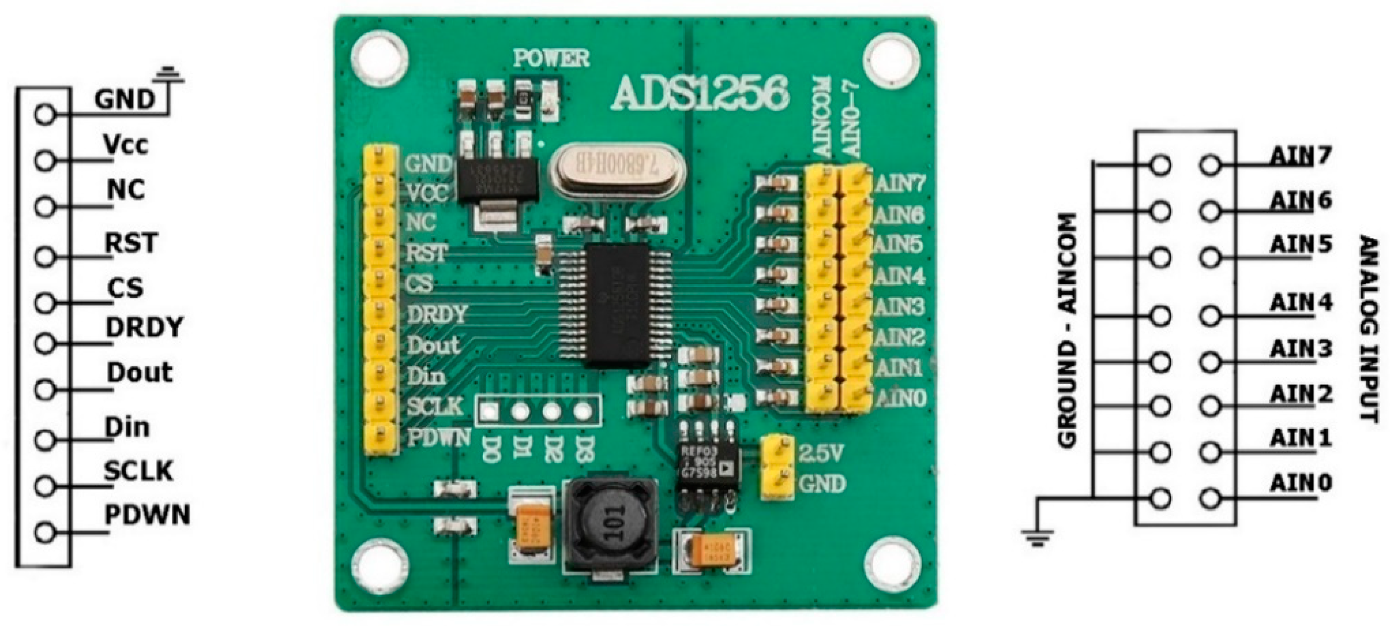
| Pin Description | ADS1256 Pin-Out | Raspberry Pi-4 Pin-Out |
|---|---|---|
| 3.3 V Power | VCC | 1 |
| Ground | GND | 6 |
| Data Ready | DRDY | 11 |
| Reset | RST | 12 |
| Power Down | PDWN | 13 |
| Chip Select | CS | 15 |
| Master Out Slave In | DIN | 19 |
| Master In Slave Out | DOUT | 21 |
| Serial Clock | SCLK | 23 |
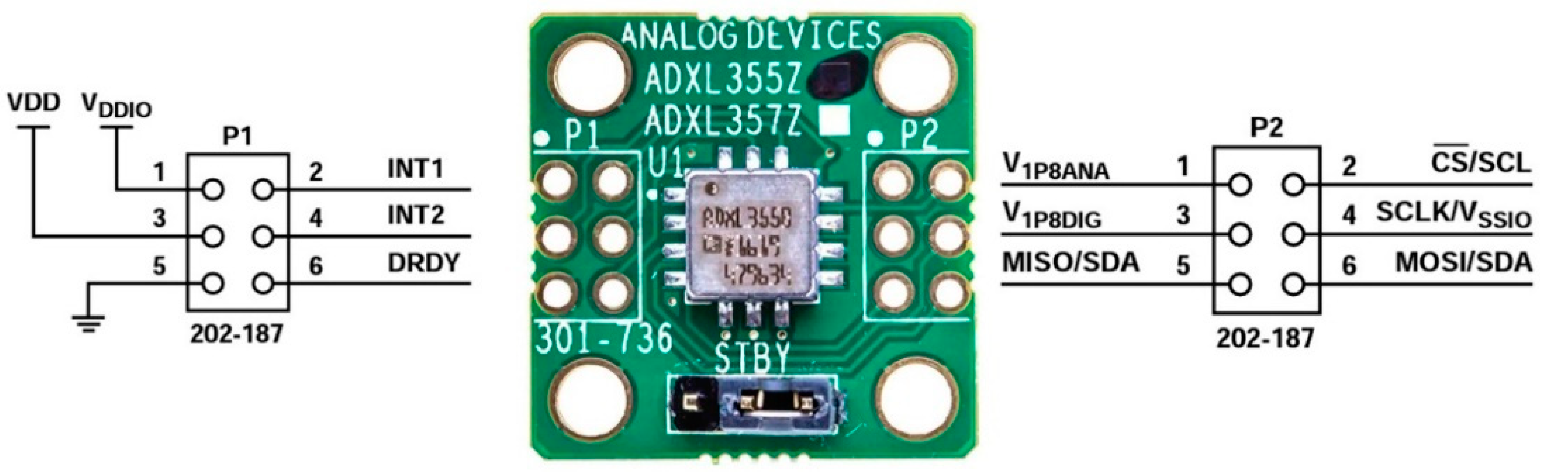
| Pin Description | ADXL355 Pin-Out | Raspberry Pi-4 Pin-Out |
|---|---|---|
| 3.3 V Digital Power | VDDIO (1) | 1 |
| 3.3 V Digital Power | VDD (3) | 1 or 17 |
| Ground | GND (5) | 9 |
| Data Ready | DRDY (6) | 11 |
| Chip Select | CS (8) | 24 |
| Serial Clock | SCLK (10) | 23 |
| Master In Slave Out | MISO (11) | 21 |
| Master Out Slave In | MOSI (12) | 19 |
| NS Direction | EW Direction | ||||
|---|---|---|---|---|---|
| 1st Mode | 2nd Mode | 1st Mode | 2nd Mode | ||
| GURALP-5TDE | 9th Floor | 0.51 | 0.151 | 0.66 | 0.193 |
| CEDAS_acc6 | 9th Floor | 0.51 | 0.151 | 0.66 | 0.193 |
| Device | Direction | Absolute Peak Values | ||
|---|---|---|---|---|
| Acceleration (mg) | Velocity (mm/s) | Displacement (mm) | ||
| GURALP-5TDE | NS | 0.611 | 0.382 | 0.026 |
| EW | 0.741 | 0.341 | 0.024 | |
| CEDAS_acc | NS | 0.607 | 0.422 | 0.041 |
| EW | 0.712 | 0.372 | 0.031 | |
Disclaimer/Publisher’s Note: The statements, opinions and data contained in all publications are solely those of the individual author(s) and contributor(s) and not of MDPI and/or the editor(s). MDPI and/or the editor(s) disclaim responsibility for any injury to people or property resulting from any ideas, methods, instructions or products referred to in the content. |
© 2024 by the authors. Licensee MDPI, Basel, Switzerland. This article is an open access article distributed under the terms and conditions of the Creative Commons Attribution (CC BY) license (https://creativecommons.org/licenses/by/4.0/).
Share and Cite
Özdemir, K.; Kömeç Mutlu, A. Cost-Effective Data Acquisition Systems for Advanced Structural Health Monitoring. Sensors 2024, 24, 4269. https://doi.org/10.3390/s24134269
Özdemir K, Kömeç Mutlu A. Cost-Effective Data Acquisition Systems for Advanced Structural Health Monitoring. Sensors. 2024; 24(13):4269. https://doi.org/10.3390/s24134269
Chicago/Turabian StyleÖzdemir, Kamer, and Ahu Kömeç Mutlu. 2024. "Cost-Effective Data Acquisition Systems for Advanced Structural Health Monitoring" Sensors 24, no. 13: 4269. https://doi.org/10.3390/s24134269
APA StyleÖzdemir, K., & Kömeç Mutlu, A. (2024). Cost-Effective Data Acquisition Systems for Advanced Structural Health Monitoring. Sensors, 24(13), 4269. https://doi.org/10.3390/s24134269