
Coupling Fault Diagnosis Based on Dynamic Vertex Interpretable Graph Neural Network


Abstract
1. Introduction
- (a)
- A topology construction method of dynamic vertex data for graph neural networks is proposed, which is suitable for topology-based correlation analysis.
- (b)
- An explainable coupling fault diagnosis method is proposed, which gives physical meaning to the data-driven method based on the graph neural network.
- (c)
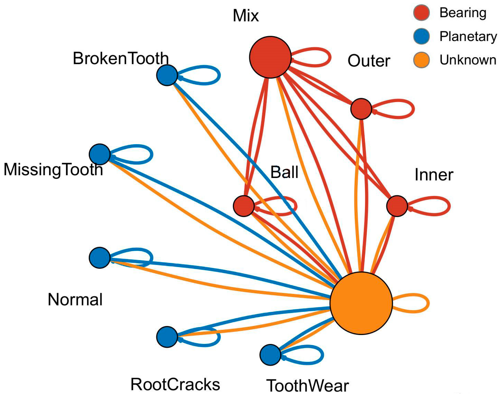
- In this paper, the bearing coupling fault was analyzed as an example, and the test results show that the method can realize coupling component analysis on the basis of coupling fault diagnosis.
2. Interpretability of Graph Neural Networks
3. Algorithm Flow
3.1. Data Preprocessing
3.2. Coupling Fault Diagnosis
3.3. Algorithm Flow
- (a)
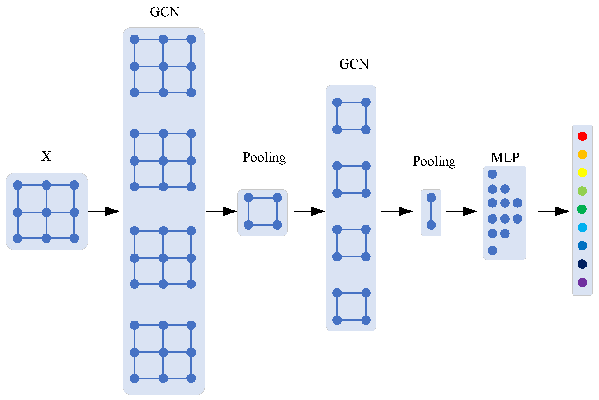
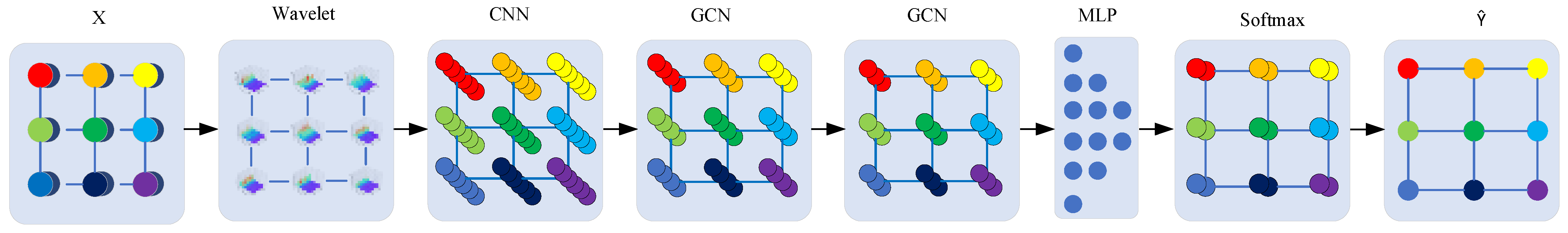
- The input data , are composed of node features of types of faults, where is the feature dimension. The node is the dynamic vertex (i.e., the fault node to be diagnosed).
- (b)
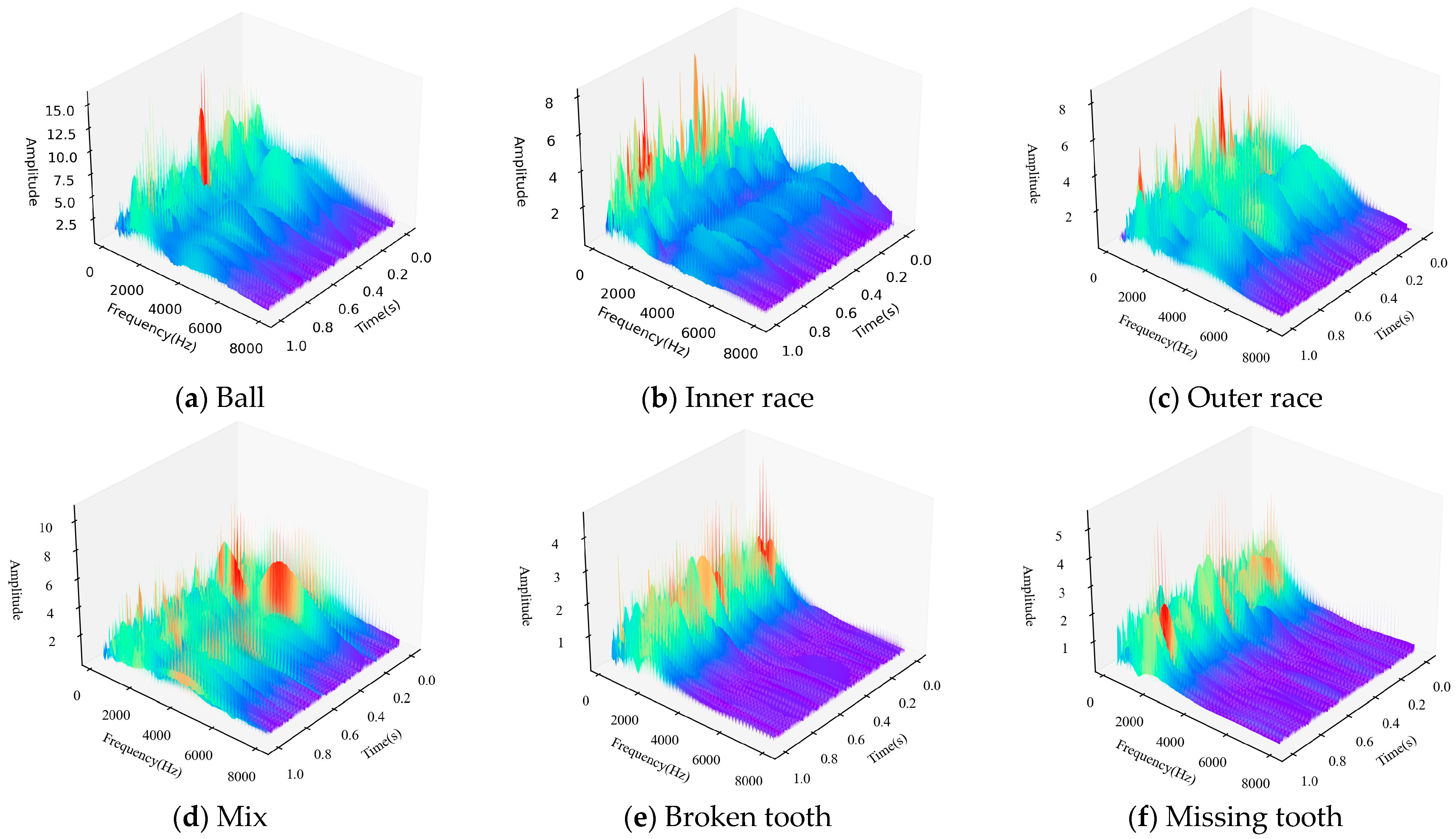
- After is transformed by wavelet, , where is the number of the frequency spectrum and is the size of the wavelet scale. The wavelet transform raises the dimension of one-dimensional data, endows the data with more intuitive features, and at the same time, carries out data preprocessing, which is conducive to the subsequent feature extraction of the neural network.
- (c)
- After the signal is convolved on the two-dimensional spectrum data, the number of convolution nuclei is , and is obtained. Through model training, it extracts the feature assignment in at each frequency and carries out standardization processing. In the process of CNN, only independent convolution processing is carried out for each node, that is, no data information from other nodes is involved.
- (d)
- Through the two-layer GCN network, it can be obtained that , , where , . The feature extraction of high-frequency and low-frequency features is further carried out in the way of dichotomy, which is similar to the wavelet packet decomposition technology [40]. At the same time, the specific features of each type of fault are extracted through model training.
- (e)
- Through the fully connected MLP, there is further dimensionality reduction of the data, , . Finally, fault classification is output through the Softmax layer.
- (f)
- In the process of model training, the output value of the last layer of node is used as the training label to optimize the model parameters. After the model is established, node will play the same role with other nodes in the model operation, which only carry out independent output in the model output phase.
3.4. Interpretability Analysis
- (a)
- Each node in is a type of fault data, and the topological structure maintains the input structure from beginning to end. Each node has a clear physical meaning, and each node in the output data corresponds to the classification of various types of fault data.
- (b)
- The vibration signal is converted into the time–frequency domain signal by wavelet transform, which provides the data with a clear physical meaning. Due to the introduction of data topology, the physical meaning of each vertex data remains stable, even if the data dimension is changed under the condition that the GCN network structure remains unchanged, and all of them are linear transformations of the vibration amplitude of this type of fault at a specific frequency.
- (c)
- The similar characteristics of similar faults in coupling faults are enhanced by aggregation operation:where , and the fault characteristic information of related nodes is aggregated through the target vertex of GCN. The nodes at both ends are comprehensively considered by the symmetric standardization operation . The degree of coupling fault is relatively large because it is related to multiple fault nodes, and the symmetric standardization can reduce the weight of such nodes in the aggregation, effectively avoiding the influence of unrelated fault type data on the aggregation of adjacent nodes.
4. Dataset Introduction and Data Processing
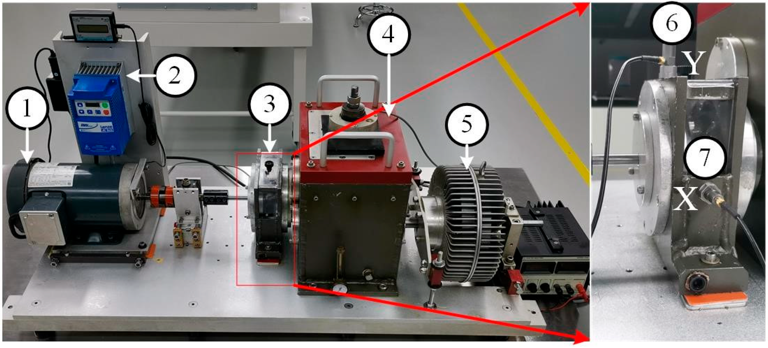
4.1. Dataset Introduction
4.2. Data Preprocessing
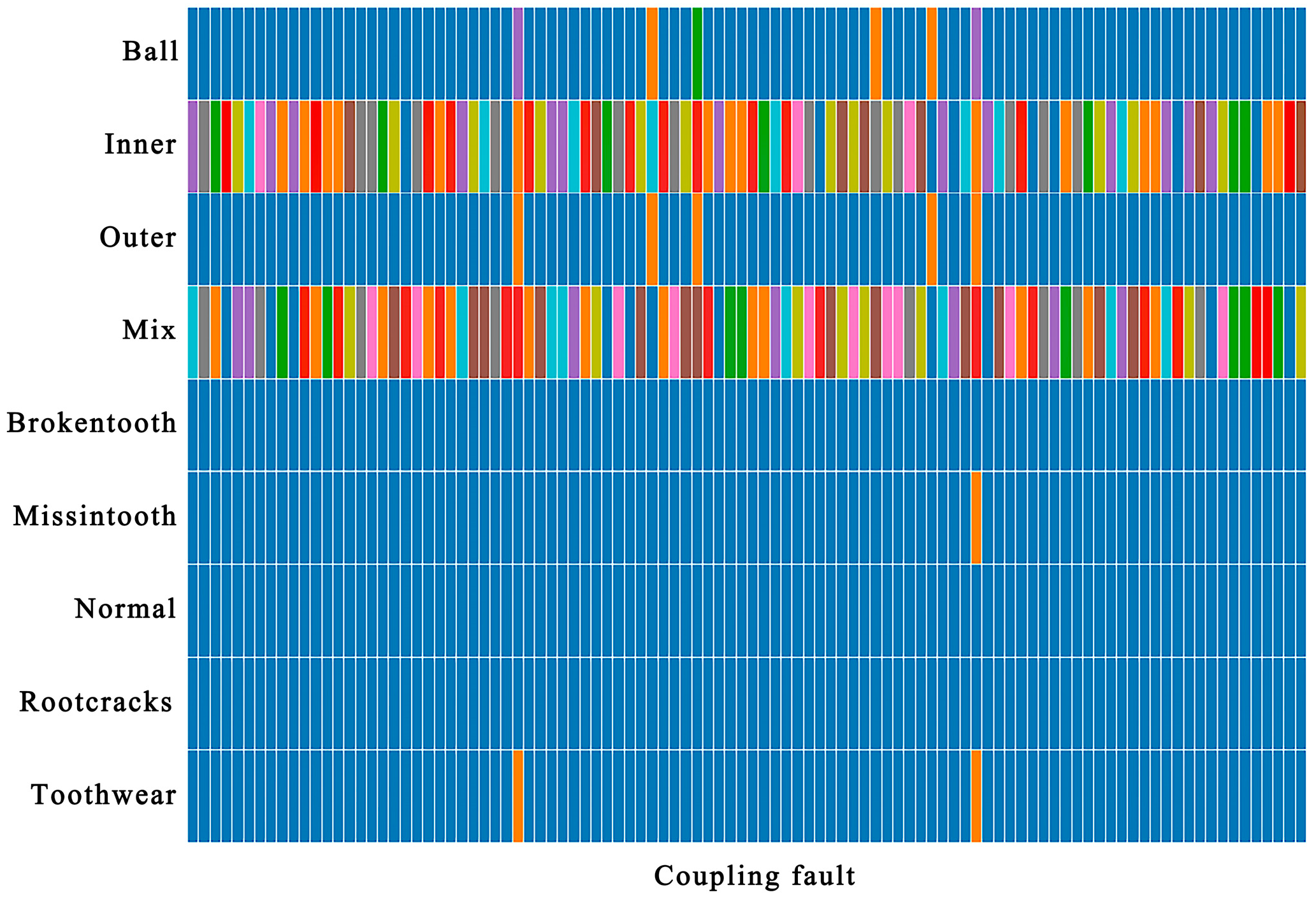
4.3. Coupling Fault Diagnosis
5. Discussion and Conclusions
Author Contributions
Funding
Data Availability Statement
Conflicts of Interest
References
- Zhu, Y.; Liang, X.; Wang, T.; Xie, J.; Yang, J. Depth Prototype Clustering Method Based on Unsupervised Field Alignment for Bearing Fault Identification of Mechanical Equipment. IEEE Trans. Instrum. Meas. 2022, 71, 1–14. [Google Scholar] [CrossRef]
- Cao, Z.; Wu, G.A.; He, C.B.; Rao, M.; Tu, W.B. A new instantaneous contact based dynamic model of rolling element bearings with local defects. Mech. Syst. Signal Process. 2023, 200, 110600. [Google Scholar] [CrossRef]
- Che, C.C.; Wang, H.W.; Lin, R.G.; Ni, X.M. Deep meta-learning and variational autoencoder for coupling fault diagnosis of rolling bearing under variable working conditions. Proc. Inst. Mech. Eng. Part C-J. Mech. Eng. Sci. 2022, 236, 9900–9913. [Google Scholar] [CrossRef]
- He, F.; Zheng, C.; Pang, C.; Zhao, C.; Yang, M.; Zhu, Y.; Luo, Z.; Luo, H.; Li, L.; Jiang, H. An Adaptive Deconvolution Method with Improve Enhanced Envelope Spectrum and Its Application for Bearing Fault Feature Extraction. Sensors 2024, 24, 951. [Google Scholar] [CrossRef] [PubMed]
- Ouyang, T.C.; Wang, G.; Cheng, L.; Wang, J.X.; Yang, R. Comprehensive diagnosis and analysis of spur gears with pitting-crack coupling faults. Mech. Mach. Theory 2022, 176, 104968. [Google Scholar] [CrossRef]
- Mishra, R.K.; Choudhary, A.; Fatima, S.; Mohanty, A.R.; Panigrahi, B.K. Multi-fault Diagnosis of Rotating Machine Under Uncertain Speed Conditions. J. Vib. Eng. Technol. 2024, 12, 4637–4654. [Google Scholar] [CrossRef]
- Tao, H.; Qiu, J.; Chen, Y.; Stojanovic, V.; Cheng, L. Unsupervised cross-domain rolling bearing fault diagnosis based on time-frequency information fusion. J. Frankl. Inst. Eng. Appl. Math. 2023, 360, 1454–1477. [Google Scholar] [CrossRef]
- Zhang, J.; Zhang, Q.; Feng, W.; Qin, X.; Sun, Y. A feature vector with insensitivity to the position of the outer race defect and its application in rolling bearing fault diagnosis. Struct. Health Monit. Int. J. 2024, in press. [Google Scholar] [CrossRef]
- Zhao, D.; Li, J.; Cheng, W.; Wen, W. Bearing multi-fault diagnosis with iterative generalized demodulation guided by enhanced rotational frequency matching under time-varying speed conditions. Isa Trans. 2023, 133, 518–528. [Google Scholar] [CrossRef]
- Neisi, N.; Nieminen, V.; Kurvinen, E.; Lämsä, V.; Sopanen, J. Estimation of Unmeasurable Vibration of a Rotating Machine Using Kalman Filter. Machines 2022, 10, 23. [Google Scholar] [CrossRef]
- Wang, C.; Peng, Z.M.; Liu, R.; Chen, C. Research on Multi-Fault Diagnosis Method Based on Time Domain Features of Vibration Signals. Sensors 2022, 22, 15. [Google Scholar] [CrossRef] [PubMed]
- RicoMartinez, R.; Anderson, J.S.; Kevrekidis, I.G. Self-consistency in neural network-based NLPC analysis with applications to time-series processing. Comput. Chem. Eng. 1996, 20, S1089–S1094. [Google Scholar] [CrossRef]
- Zhang, X.; Li, J.; Wu, W.; Dong, F.; Wan, S. Multi-Fault Classification and Diagnosis of Rolling Bearing Based on Improved Convolution Neural Network. Entropy 2023, 25, 737. [Google Scholar] [CrossRef]
- Gong, X.Y.; Feng, K.P.; Du, W.L.; Li, B.S.; Fei, H.Y. An imbalance multi-faults data transfer learning diagnosis method based on finite element simulation optimization model of rolling bearing. Proc. Inst. Mech. Eng. Part C-J. Mech. Eng. Sci. 2024, 17, 09544062241245826. [Google Scholar] [CrossRef]
- Deng, J.; Liu, H.; Fang, H.; Shao, S.; Wang, D.; Hou, Y.; Chen, D.; Tang, M. MgNet: A fault diagnosis approach for multi-bearing system based on auxiliary bearing and multi-granularity information fusion. Mech. Syst. Signal Process. 2023, 193, 110253. [Google Scholar] [CrossRef]
- Shi, L.; Su, S.; Wang, W.; Gao, S.; Chu, C. Bearing Fault Diagnosis Method Based on Deep Learning and Health State Division. Appl. Sci. 2023, 13, 7424. [Google Scholar] [CrossRef]
- Hadi, R.H.; Hady, H.N.; Hasan, A.M.; Al-Jodah, A.; Humaidi, A.J. Improved Fault Classification for Predictive Maintenance in Industrial IoT Based on AutoML: A Case Study of Ball-Bearing Faults. Processes 2023, 11, 1507. [Google Scholar] [CrossRef]
- Xu, J.; Kong, H.; Li, K.; Ding, X. Generative Zero-Shot Compound Fault Diagnosis Based on Semantic Alignment. IEEE Trans. Instrum. Meas. 2024, 73, 13. [Google Scholar] [CrossRef]
- Zhang, Y.; Tino, P.; Leonardis, A.; Tang, K. A Survey on Neural Network Interpretability. IEEE Trans. Emerg. Top. Comput. Intell. 2021, 5, 726–742. [Google Scholar] [CrossRef]
- Li, H.; Lin, J.; Liu, Z.; Jiao, J.; Zhang, B. An interpretable waveform segmentation model for bearing fault diagnosis. Adv. Eng. Inform. 2024, 61, 102480. [Google Scholar] [CrossRef]
- Che, C.; Zhang, Y.; Wang, H.; Xiong, M. Interpretable multi-domain meta-transfer learning for few-shot fault diagnosis of rolling bearing under variable working conditions. Meas. Sci. Technol. 2024, 35, 076103. [Google Scholar] [CrossRef]
- Scarselli, F.; Gori, M.; Tsoi, A.C.; Hagenbuchner, M.; Monfardini, G. The Graph Neural Network Model. IEEE Trans. Neural Netw. 2009, 20, 61–80. [Google Scholar] [CrossRef] [PubMed]
- Wang, Y.Q.; Li, C.Z.; Liu, Z.; Li, M.Z.; Tang, J.L.; Xie, X.; Chen, L.; Yu, P.S. An Adaptive Graph Pre-training Framework for Localized Collaborative Filtering. ACM Trans. Inf. Syst. 2023, 41, 27. [Google Scholar] [CrossRef]
- Wang, Y.Z.; Wang, C.X.; Zhan, J.Y.; Ma, W.J.; Jiang, Y.C. Text FCG: Fusing Contextual Information via Graph Learning for text classification. Expert Syst. Appl. 2023, 219, 10. [Google Scholar] [CrossRef]
- Zhang, C.H.; Zhang, S.Y.; Yu, J.J.Q.; Yu, S. FASTGNN: A Topological Information Protected Federated Learning Approach for Traffic Speed Forecasting. IEEE Trans. Ind. Inform. 2021, 17, 8464–8474. [Google Scholar] [CrossRef]
- Sharma, A.; Sharma, A.; Nikashina, P.; Gavrilenko, V.; Tselykh, A.; Bozhenyuk, A.; Masud, M.; Meshref, H. A Graph Neural Network (GNN)-Based Approach for Real-Time Estimation of Traffic Speed in Sustainable Smart Cities. Sustainability 2023, 15, 25. [Google Scholar] [CrossRef]
- Le, N.Q.K. Predicting emerging drug interactions using GNNs. Nat. Comput. Sci. 2023, 3, 1007–1008. [Google Scholar] [CrossRef] [PubMed]
- Zhang, Y.; Yao, Q.; Yue, L.; Wu, X.; Zhang, Z.; Lin, Z.; Zheng, Y. Emerging drug interaction prediction enabled by a flow-based graph neural network with biomedical network. Nat. Comput. Sci. 2023, 3, 1023–1033. [Google Scholar] [CrossRef] [PubMed]
- Bruna, J.; Zaremba, W.; Szlam, A.; LeCun, Y. Spectral Networks and Locally Connected Networks on Graphs. arXiv 2013, arXiv:1312.6203. [Google Scholar] [CrossRef]
- Defferrard, M.; Bresson, X.; Vandergheynst, P. Convolutional Neural Networks on Graphs with Fast Localized Spectral Filtering. In Proceedings of the Neural Information Processing Systems, Barcelona, Spain, 5–10 December 2016. [Google Scholar]
- Gama, F.; Marques, A.G.; Leus, G.; Ribeiro, A. Convolutional Neural Network Architectures for Signals Supported on Graphs. IEEE Trans. Signal Process. 2019, 67, 1034–1049. [Google Scholar] [CrossRef]
- Li, T.; Zhou, Z.; Li, S.; Sun, C.; Yan, R.; Chen, X. The emerging graph neural networks for intelligent fault diagnostics and prognostics: A guideline and a benchmark study. Mech. Syst. Signal Process. 2022, 168, 108653. [Google Scholar] [CrossRef]
- Gao, Y.; Wu, H.; Liao, H.; Chen, X.; Yang, S.; Song, H. A fault diagnosis method for rolling bearings based on graph neural network with one-shot learning. Eurasip J. Adv. Signal Process. 2023, 2023, 101. [Google Scholar] [CrossRef]
- Man, J.; Dong, H.; Jia, L.; Qin, Y.; Zhang, J. An Adaptive Multisensor Fault Diagnosis Method for High-Speed Train Bogie. IEEE Trans. Intell. Transp. Syst. 2023, 24, 6292–6306. [Google Scholar] [CrossRef]
- Zhang, Z.; Wu, L. Graph neural network-based bearing fault diagnosis using Granger causality test. Expert Syst. Appl. 2024, 242, 122827. [Google Scholar] [CrossRef]
- Zhang, H.Q.; Lu, G.Q.; Zhan, M.M.; Zhang, B.X. Semi-Supervised Classification of Graph Convolutional Networks with Laplacian Rank Constraints. Neural Process. Lett. 2022, 54, 2645–2656. [Google Scholar] [CrossRef]
- Wu, Z.; Pan, S.; Chen, F.; Long, G.; Zhang, C.; Yu, P.S. A Comprehensive Survey on Graph Neural Networks. IEEE Trans. Neural Netw. Learn. Syst. 2021, 32, 4–24. [Google Scholar] [CrossRef]
- Peng, P.; Lu, J.X.; Xie, T.Y.; Tao, S.T.; Wang, H.W.; Zhang, H.M. Open-Set Fault Diagnosis via Supervised Contrastive Learning with Negative Out-of-Distribution Data Augmentation. IEEE Trans. Ind. Inform. 2023, 19, 2463–2473. [Google Scholar] [CrossRef]
- Shao, S.Y.; Yan, R.Q.; Lu, Y.D.; Wang, P.; Gao, R.X. DCNN-Based Multi-Signal Induction Motor Fault Diagnosis. IEEE Trans. Instrum. Meas. 2020, 69, 2658–2669. [Google Scholar] [CrossRef]
- Cao, D.X.; Gu, Y.; Lin, W. Fault diagnosis based on optimized wavelet packet transform and time domain convolution network. Trans. FAMENA 2023, 47, 1–14. [Google Scholar] [CrossRef]
- Li, X.; Xiong, H.; Li, X.; Wu, X.; Zhang, X.; Liu, J.; Bian, J.; Dou, D. Interpretable deep learning: Interpretation, interpretability, trustworthiness, and beyond. Knowl. Inf. Syst. 2022, 64, 3197–3234. [Google Scholar] [CrossRef]
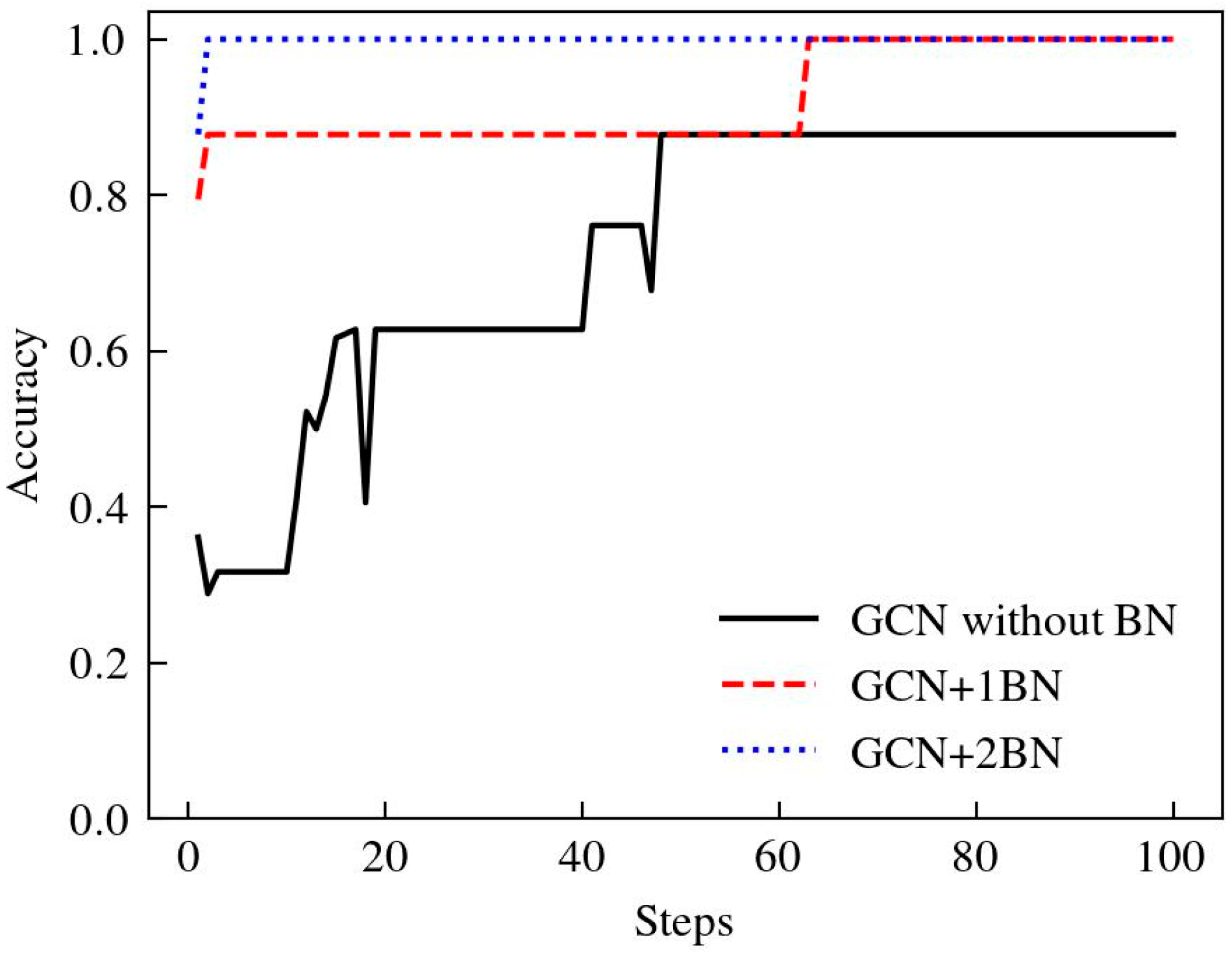
- Takagi, S.; Yoshida, Y.; Okada, M. The Effect of Batch Normalization in the Symmetric Phase. In Proceedings of the Artificial Neural Networks and Machine Learning, ICANN 2020, PT II, Bratislava, Slovakia, 15–18 September 2020; pp. 229–240. [Google Scholar]


| Notions | Descriptions |
|---|---|
| Graph data | |
| Vertex set | |
| Edge set | |
| Adjacent matrix | |
| Adjacent matrix with self-loop | |
| Degree matrix | |
| Graph convolution operation | |
| Hadamar product | |
| Laplacian matrix | |
| Fourier basis matrix of | |
| Eigenvalue matrix of | |
| Eigenvalue forms | |
| Feature matrix of a graph | |
| , | The feature vector of a graph |
| True label of | |
| Predicted label of | |
| Filter parameterized by | |
| Chebyshev polynomial coefficients | |
| Nonlinear activation function | |
| , | Learnable model parameters |
| Family of wavelets | |
| Weight of the loss function | |
| Diagnosis accuracy of coupled fault | |
| Comprehensive diagnosis accuracy of coupling faults |
| Models | Validation Accuracy | Test Accuracy | Steps to Convergence |
|---|---|---|---|
| ChebyNet | 90.56% | 82.78% | 7 |
| GCN | 98.33% | 98.89% | / |
| WLChebyNet | 100% | 96.67% | 29 |
| WLHOGNN | 100% | 99.45% | 10 |
| WLGraphSAGE | 100% | 97.8% | 8 |
| DIGNN | 100% | 100% | 2 |
| Fault Mode | Inner | Ball | Outer |
|---|---|---|---|
| 1st obvious fault | 100% | 0 | 0 |
| 2nd obvious fault | 0 | 94% | 6% |
| 3rd obvious fault | 0 | 6% | 59% |
| Coupling fault diagnosis accuracy | 100% | 100% | 65% |
| Comprehensive accuracy | 88.3% | ||
Disclaimer/Publisher’s Note: The statements, opinions and data contained in all publications are solely those of the individual author(s) and contributor(s) and not of MDPI and/or the editor(s). MDPI and/or the editor(s) disclaim responsibility for any injury to people or property resulting from any ideas, methods, instructions or products referred to in the content. |
© 2024 by the authors. Licensee MDPI, Basel, Switzerland. This article is an open access article distributed under the terms and conditions of the Creative Commons Attribution (CC BY) license (https://creativecommons.org/licenses/by/4.0/).
Share and Cite
Wang, S.; Jing, B.; Pan, J.; Meng, X.; Huang, Y.; Jiao, X. Coupling Fault Diagnosis Based on Dynamic Vertex Interpretable Graph Neural Network. Sensors 2024, 24, 4356. https://doi.org/10.3390/s24134356
Wang S, Jing B, Pan J, Meng X, Huang Y, Jiao X. Coupling Fault Diagnosis Based on Dynamic Vertex Interpretable Graph Neural Network. Sensors. 2024; 24(13):4356. https://doi.org/10.3390/s24134356
Chicago/Turabian StyleWang, Shenglong, Bo Jing, Jinxin Pan, Xiangzhen Meng, Yifeng Huang, and Xiaoxuan Jiao. 2024. "Coupling Fault Diagnosis Based on Dynamic Vertex Interpretable Graph Neural Network" Sensors 24, no. 13: 4356. https://doi.org/10.3390/s24134356
APA StyleWang, S., Jing, B., Pan, J., Meng, X., Huang, Y., & Jiao, X. (2024). Coupling Fault Diagnosis Based on Dynamic Vertex Interpretable Graph Neural Network. Sensors, 24(13), 4356. https://doi.org/10.3390/s24134356