
Piezoelectric Transducers: Complete Electromechanical Model with Parameter Extraction
Abstract
:1. Introduction
2. Complete Electromechanical Model
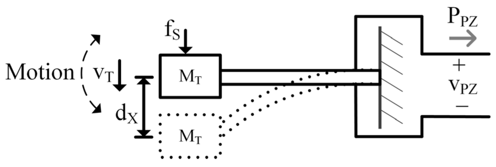
2.1. Complete Model
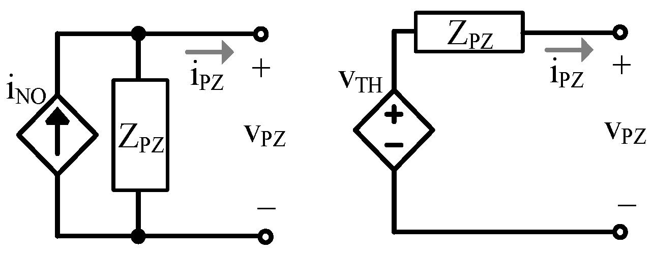
2.2. Electrical Model
2.3. Lumped Electrical Model
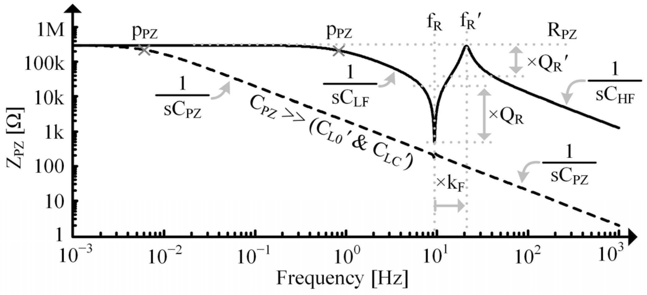
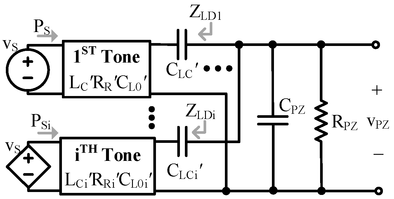
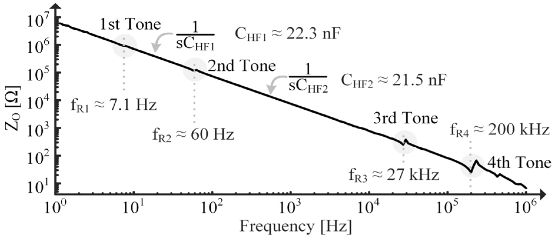
2.4. Additional Resonant Tones
3. Electromechanical Coupling
3.1. Coupling Coefficients
3.2. Coupling Extremes
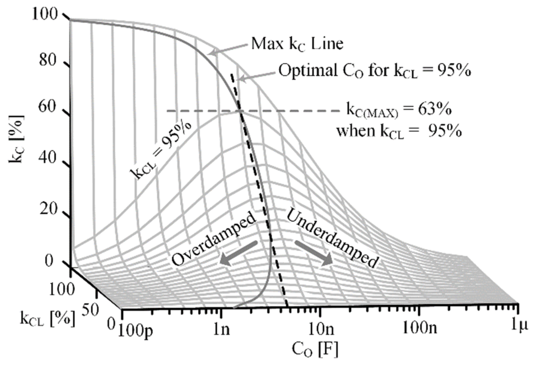
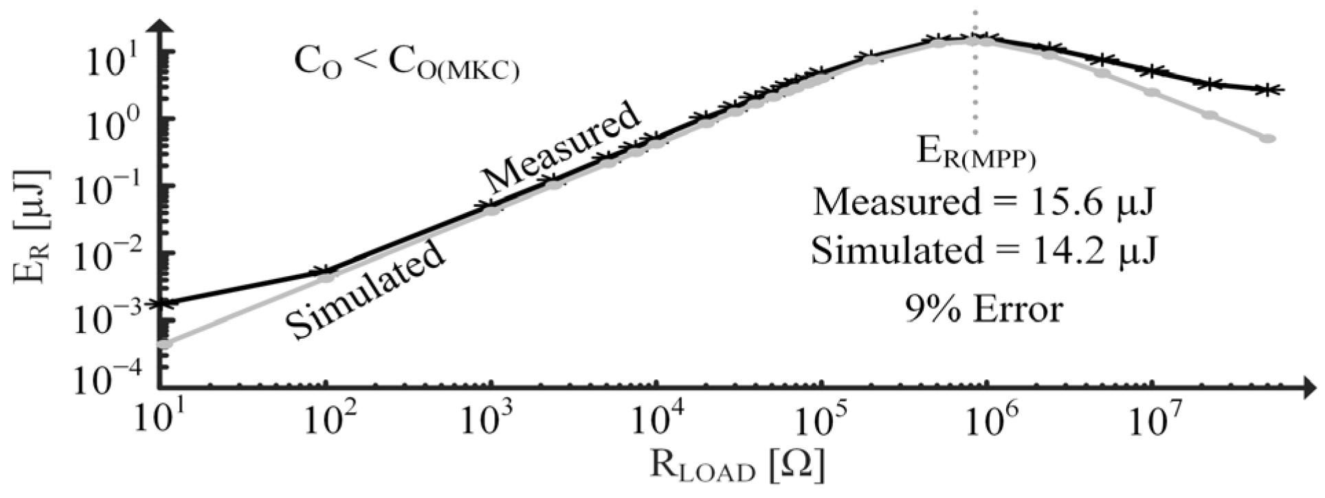
3.3. Coupling with a Capacitive Load
4. Parameter Extraction
4.1. Mechanical Parameters
4.2. Electrical Parameters
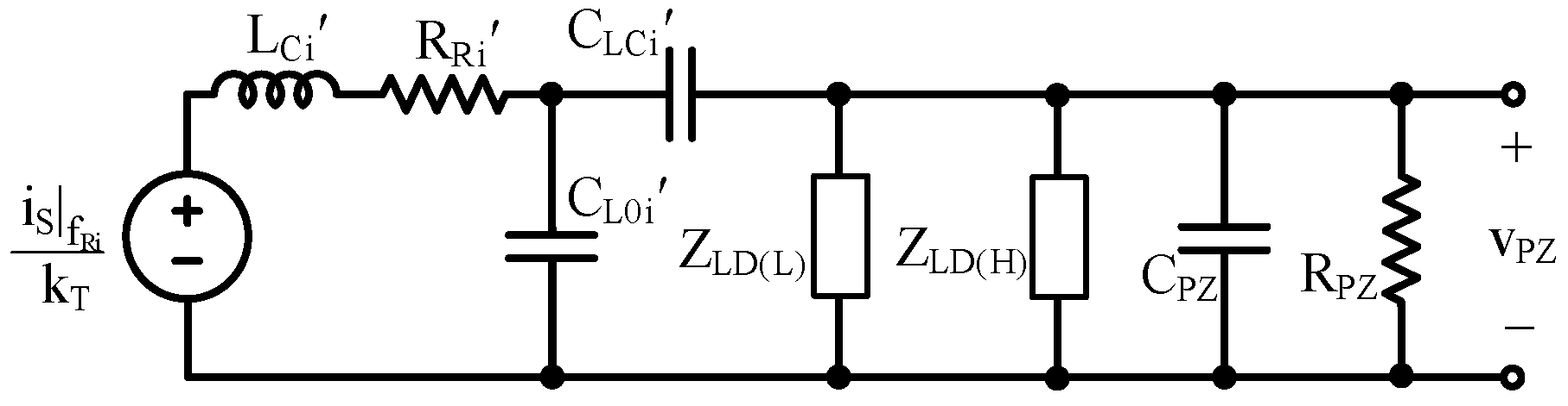
4.3. Approximating 2nd Tone
5. Model Validation
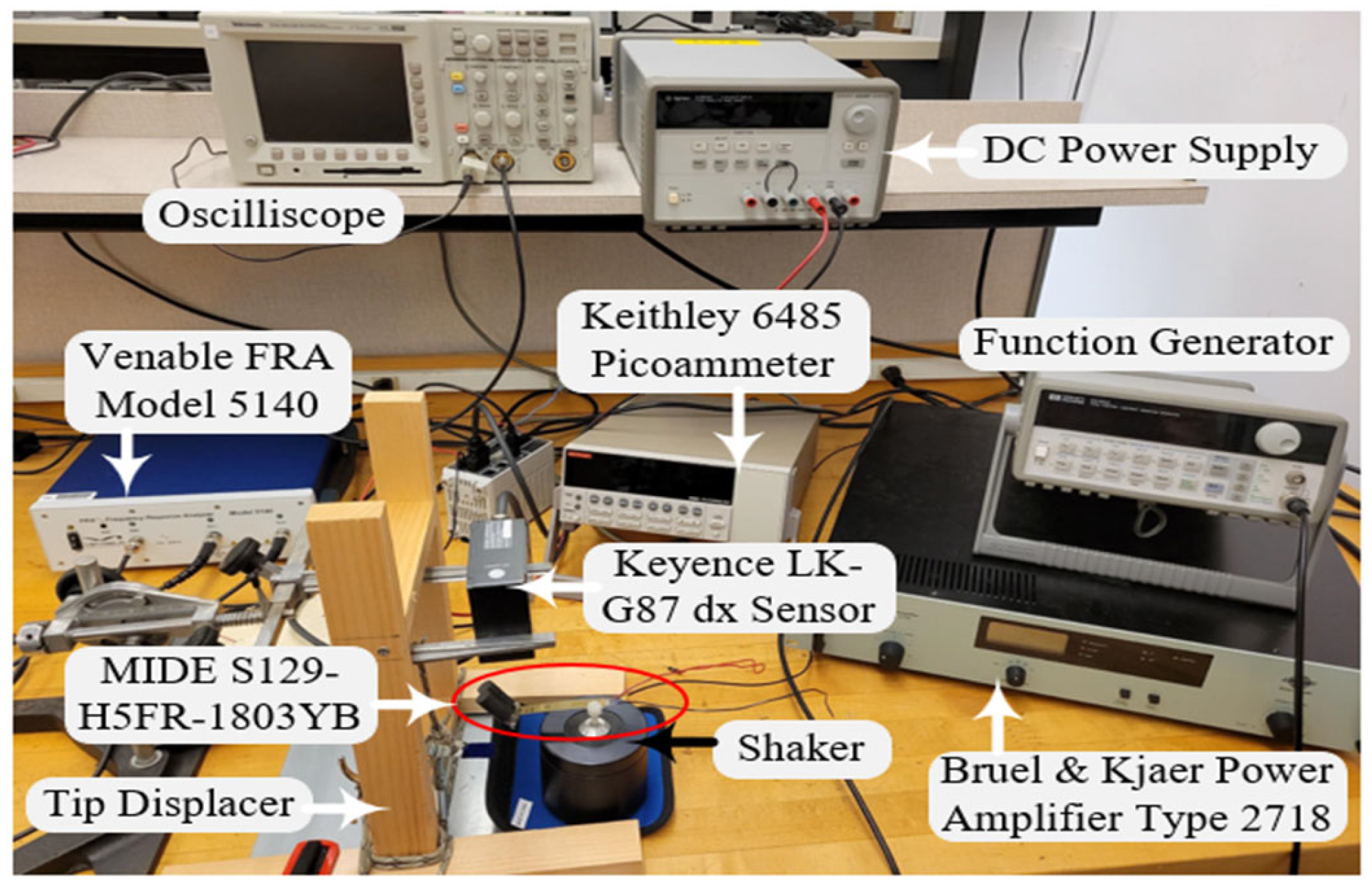
5.1. Test Setup
5.2. Parameter Extraction
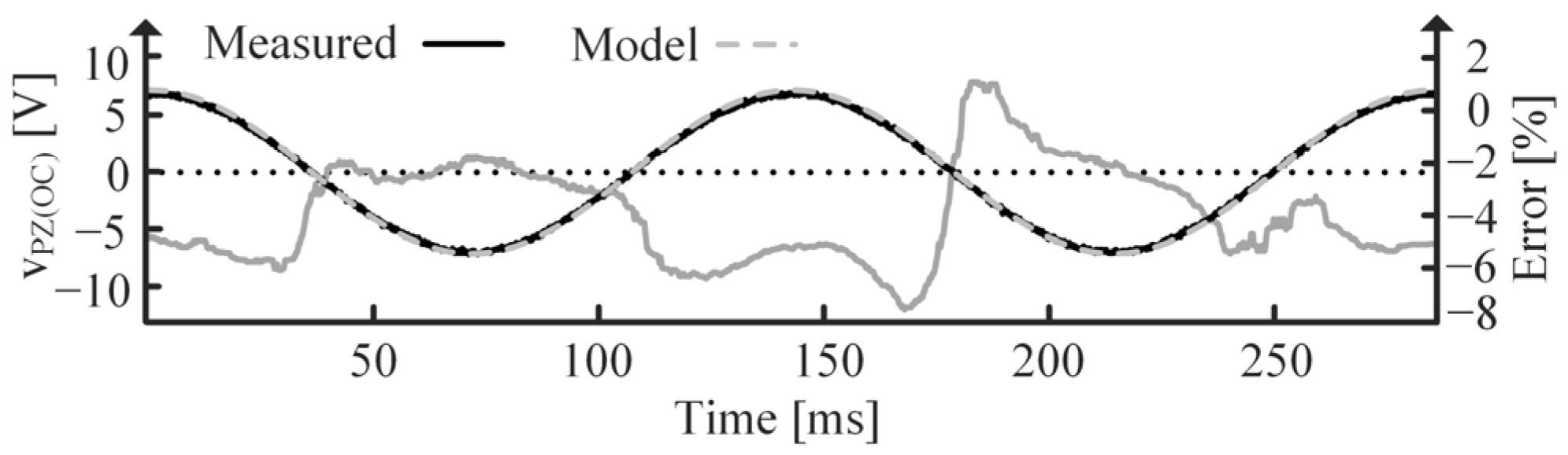
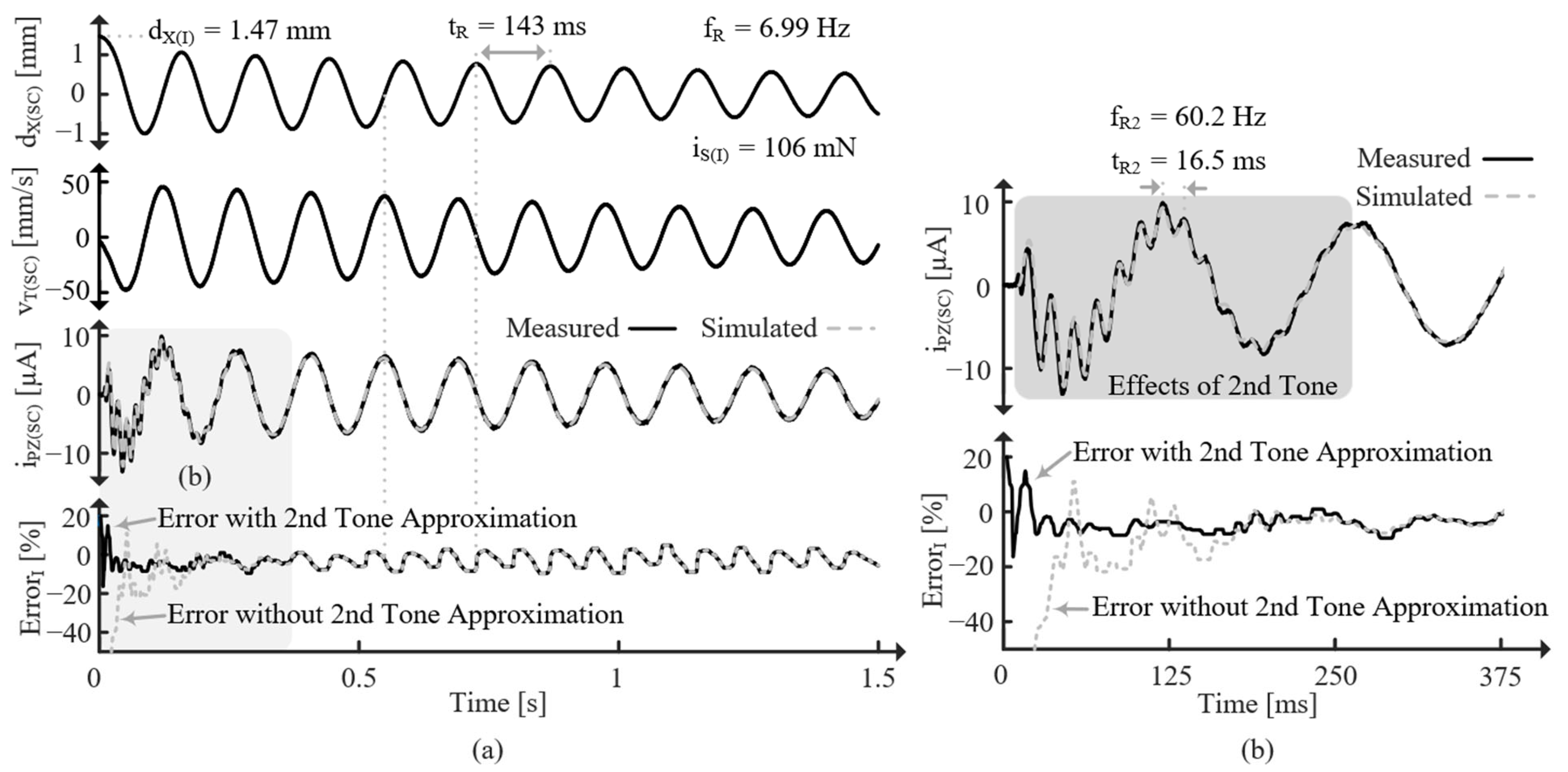
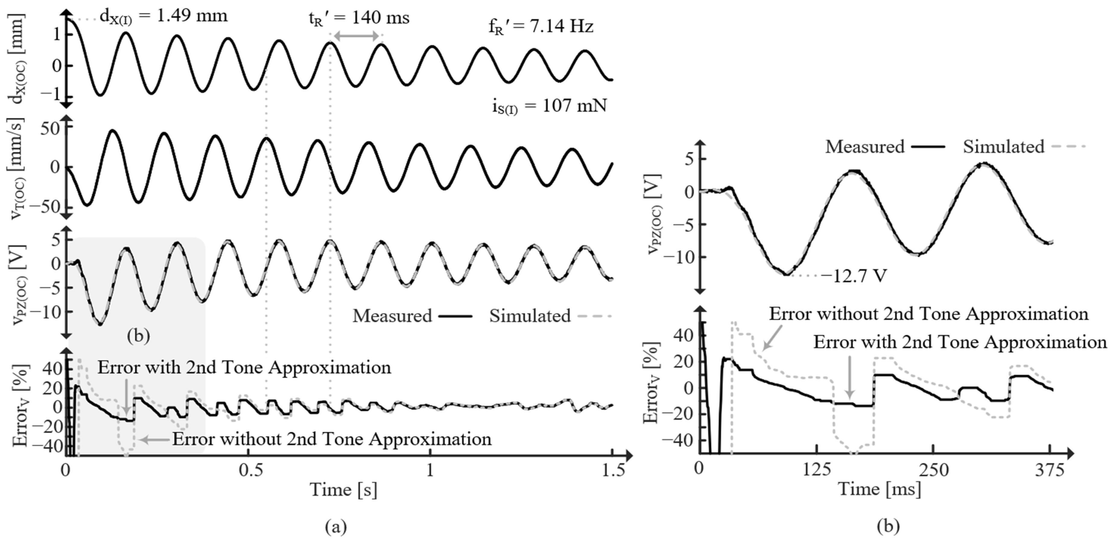
5.3. Resonant Vibrations
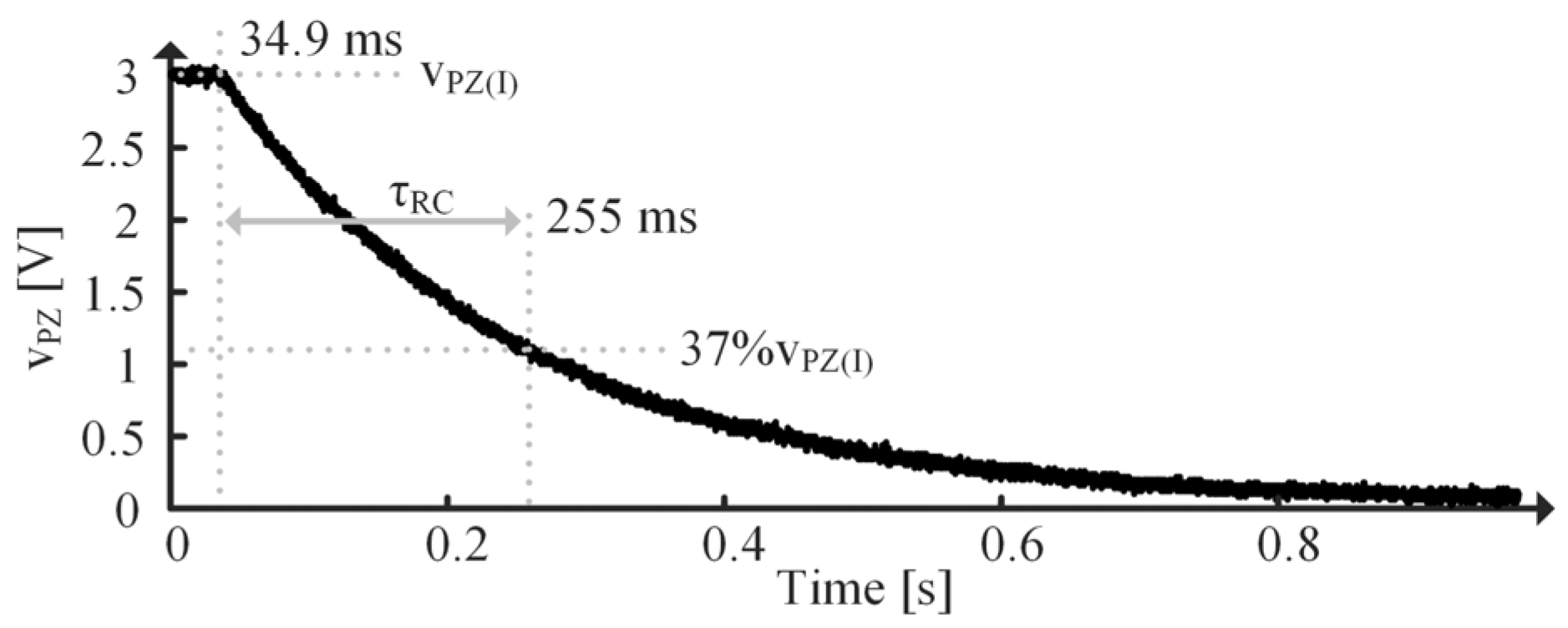
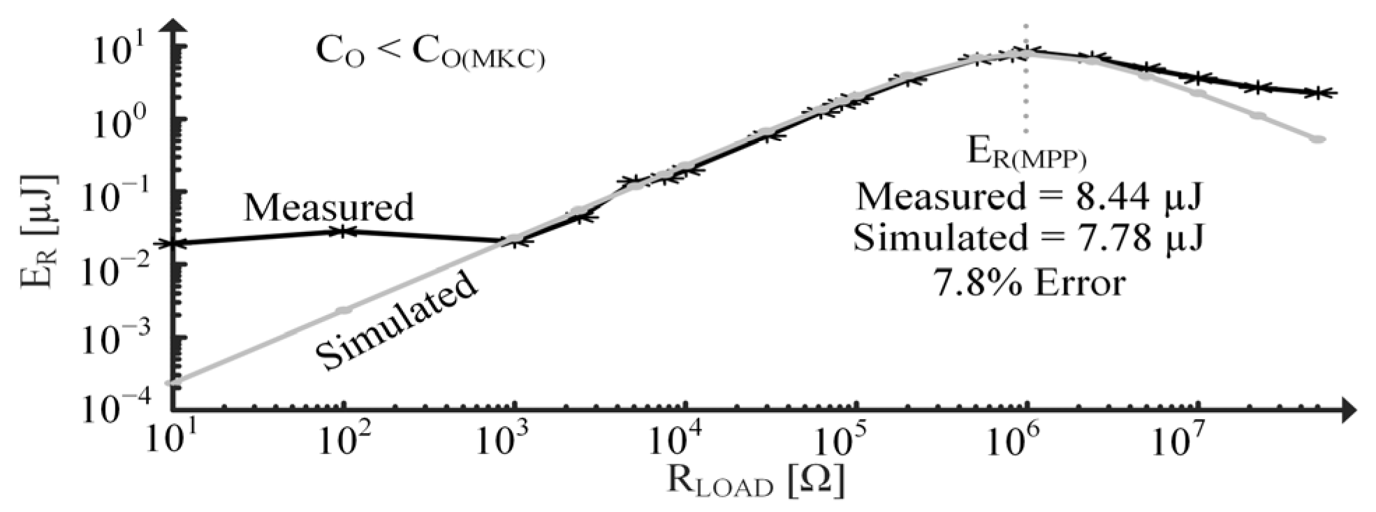
5.4. Step Response
6. Conclusions
Author Contributions
Funding
Institutional Review Board Statement
Informed Consent Statement
Data Availability Statement
Conflicts of Interest
References
- Covaci, C.; Gontean, A. Piezoelectric Energy Harvesting Solutions: A Review. Sensors 2020, 20, 3512. [Google Scholar] [CrossRef]
- Ju, S.; Ji, C. Indirect impact based piezoelectric energy harvester for low frequency vibration. In Proceedings of the 2015 IEEE Transducers—18th International Conference on Solid-State Sensors, Actuators and Microsyst, Anchorage, AK, USA, 21–25 June 2015; pp. 1913–1916. [Google Scholar]
- Deterre, M.; Lefeuvre, E.; Zhu, Y.; Woytasik, M.; Boutaud, B.; Molin, R.D. Micro Blood Pressure Energy Harvester for Intracardiac Pacemaker. J. Microelectromech. Syst. 2014, 23, 651–660. [Google Scholar] [CrossRef]
- Li, H.; Tian, C.; Deng, Z.D. Energy harvesting from low frequency applications using piezoelectric materials. Appl. Phys. Rev. 2014, 1, 041301. [Google Scholar] [CrossRef]
- Song, H.C.; Kumar, P.; Maurya, D.; Kang, M.G.; Reynolds, W.T.; Jeong, D.Y.; Kang, C.Y.; Priya, S. Ultra-Low Resonant Piezoelectric MEMS Energy Harvester with High Power Density. J. Microelectromech. Syst. 2017, 26, 1226–1234. [Google Scholar] [CrossRef]
- Li, X.; Rincon-Mora, G.A. Maximum power-point theory for thermoelectric harvesters. In Proceedings of the 2023 IEEE 66th Midwest Symposium on Circuits and Systems, Tempe, AZ, USA, 6–9 August 2023; pp. 409–413. [Google Scholar]
- Rincón-Mora, G.A.; Yang, S. Tiny piezoelectric harvesters: Principles, constraints, and power conversion. IEEE Trans. Circ. Syst. I 2016, 63, 639–649. [Google Scholar] [CrossRef]
- Guyomar, D.; Badel, A.; Lefeuvre, E.; Richard, C. Toward energy harvesting using active materials and conversion improvement by nonlinear processing. IEEE Trans. Ultrason. Ferroelectr. Freq. Control 2005, 52, 584–595. [Google Scholar] [CrossRef]
- Erturk, A.; Inman, D.J. A distributed parameter electromechanical model for Cantilevered Piezoelectric Energy Harvesters. J. Vib. Acoust. 2008, 130, 041002. [Google Scholar] [CrossRef]
- Elvin, N.G.; Elvin, A.A. A general equivalent circuit model for piezoelectric generators. J. Intell. Mater. Syst. Struct. 2008, 20, 3–9. [Google Scholar] [CrossRef]
- Yang, Y.; Tang, L. Equivalent Circuit Modeling of Piezoelectric Energy Harvesters. J. Intell. Mater. Syst. Struct. 2009, 20, 2223–2235. [Google Scholar] [CrossRef]
- Pollet, B.; Despesse, G.; Costa, F. A New Non-Isolated Low-Power Inductorless Piezoelectric DC–DC Converter. IEEE Trans. Power Electron. 2019, 34, 11002–11013. [Google Scholar] [CrossRef]
- Boles, J.D.; Piel, J.J.; Perreault, D.J. Enumeration and Analysis of DC–DC Converter Implementations Based on Piezoelectric Resonators. IEEE Trans. Power Elect. 2021, 36, 129–145. [Google Scholar] [CrossRef]
- Pereira, L.d.A.; Morel, A.; Touhami, M.; Lamorelle, T.; Despesse, G.; Pillonnet, G. Operating Frequency Prediction of Piezoelectric DC–DC Converters. IEEE Trans. Power Electron. 2022, 37, 2508–2512. [Google Scholar] [CrossRef]
- Boles, J.D.; Bonavia, J.E.; Lang, J.H.; Perreault, D.J. A Piezoelectric-Resonator-Based DC–DC Converter Demonstrating 1 kW/cm Resonator Power Density. IEEE Trans. Power Electron. 2023, 38, 2811–2815. [Google Scholar] [CrossRef]
- Edla, M.; Lim, Y.Y.; Mikio, D.; Padilla, R.V. A Single-Stage Rectifier-Less Boost Converter Circuit for Piezoelectric Energy Harvesting Systems. IEEE Trans. Energy Convers. 2022, 37, 505–514. [Google Scholar] [CrossRef]
- Oh, T.; Islam, S.K.; To, G.; Mahfouz, M. Powering wearable sensors with a low-power CMOS piezoelectric energy harvesting circuit. In Proceedings of the 2017 IEEE International Symposium on Medical Measurements and Applications, Rochester, MN, USA, 7–10 May 2017; pp. 308–313. [Google Scholar]
- Yang, S.; Rincón-Mora, G.A. Energy-Harvesting Piezoelectric-Powered CMOS Series Switched-Inductor Bridge. IEEE Trans. Power Electron. 2019, 34, 6489–6497. [Google Scholar] [CrossRef]
- Yang, S.; Rincón-Mora, G.A. Efficient Power Transfers in Piezoelectric Energy-Harvesting Switched-Inductor Chargers. IEEE Trans. Circuits Syst. II Express Briefs 2021, 68, 1248–1252. [Google Scholar] [CrossRef]
- Roy, S.; Azad, A.N.M.W.; Baidya, S.; Khan, F. A Comprehensive Review on Rectifiers, Linear Regulators, and Switched-Mode Power Processing Techniques for Biomedical Sensors and Implants Utilizing in-Body Energy Harvesting and External Power Delivery. IEEE Trans. Power Electron. 2021, 36, 12721–12745. [Google Scholar] [CrossRef]
- Van Dyke, K.S. The Piezo-Electric Resonator and Its Equivalent Network. Proc. Inst. Radio Eng. 1928, 16, 742–764. [Google Scholar] [CrossRef]
- Friswell, M.I.; Ali, S.F.; Bilgen, O.; Adhikari, S.; Lees, A.W.; Litak, G. Non-linear piezoelectric vibration energy harvesting from a vertical cantilever beam with tip mass. J. Intell. Mater. Syst. Struct. 2012, 23, 1505–1521. [Google Scholar] [CrossRef]
- Hongjin, W.; Qingfeng, M.; Wuwei, F. Discussion of the Improved Methods for Analyzing a Cantilever Beam Carrying a Tip-Mass under Base Excitation. Shock Vib. 2014, 2014, 981053. [Google Scholar] [CrossRef]
- Isaf, M.L.; Rincon-Mora, G.A. Piezoelectric transducers for energy harvesting: Electromechanical model, ambient motion, and electrical loads. In Proceedings of the 2022 29th IEEE International Conference on Electronics, Circuits and Systems, Glasgow, UK, 24–26 October 2022; pp. 1–4. [Google Scholar]
- Arnau, A.; Soares, D. Fundamentals of Piezoelectricity. In Piezoelectric Transducers and Applications; Vives, A.A., Ed.; Springer: Berlin/Heidelberg, Germany, 2009. [Google Scholar]
- Shaarbafi, K. Transformer Modelling Guide; Teshmont Consultants LP: Winnipeg, MB, Canada, 2014. [Google Scholar]
- Kim, S.B.; Park, J.H.; Kim, S.H.; Ahn, H.; Wikle, H.C.; Kim, D.J. Modeling and Evaluation of d33 Mode Piezoelectric Energy Harvesters. J. Micromech. Microeng. 2012, 22, 105013. [Google Scholar] [CrossRef]
- Rincon-Mora, G.A. Switched Inductor Power IC Design; Springer Nature: New York, NY, USA, 2022. [Google Scholar]
- Kim, S.-B.; Park, H.; Kim, S.-H.; Wikle, H.C.; Park, J.-H.; Kim, D.-J. Comparison of MEMS PT Cantilevers Based on d31 and d33 Modes for Vibration Energy Harvesting. J. Microelectromech. Syst. 2013, 22, 26–33. [Google Scholar] [CrossRef]
- Ewins, D.J. Mode of Vibration. In Encyclopedia of Vibration; Elsevier: Amsterdam, The Netherlands, 2001; pp. 838–844. [Google Scholar]
- Lustig, S.; Elata, D. Ambiguous definitions of the piezoelectric coupling factor. J. Intell. Mater. Syst. Struct. 2020, 31, 1689–1696. [Google Scholar] [CrossRef]
- Kirkham, H.; Riepnieks, A. Students’ simple method for determining the parameters of an AC signal. In Proceedings of the 2016 57th International Scientific Conference on Power and Electrical Engineering of Riga Tech University, Riga, Latvia, 13–14 October 2016. [Google Scholar]
- Alhanaty, M.; Bercovier, M. Curve fitting and design by optimal control methods. In Proceedings of the 1998 IEEE Conference on Information Visualization, London, UK, 31 July 1998. [Google Scholar]
- Close, C.M. Modelling and Analysis of Dynamic Systems; Houghton Mifflin Company: Boston, MA, USA, 1993. [Google Scholar]


| Variable | Value |
|---|---|
| 36.0 mF | |
| 13.9 mH | |
| 32.3 Ω | |
| 16.4% | |
| 993 µ | |
| 20.4 nF | |
| 11.3 MΩ | |
| 60 Hz |
| Variable | Value |
|---|---|
| 1.0 mF | |
| 6.9 mH | |
| 54.5 Ω | |
| 45.0% | |
Disclaimer/Publisher’s Note: The statements, opinions and data contained in all publications are solely those of the individual author(s) and contributor(s) and not of MDPI and/or the editor(s). MDPI and/or the editor(s) disclaim responsibility for any injury to people or property resulting from any ideas, methods, instructions or products referred to in the content. |
© 2024 by the authors. Licensee MDPI, Basel, Switzerland. This article is an open access article distributed under the terms and conditions of the Creative Commons Attribution (CC BY) license (https://creativecommons.org/licenses/by/4.0/).
Share and Cite
Isaf, M.L.; Rincón-Mora, G.A. Piezoelectric Transducers: Complete Electromechanical Model with Parameter Extraction. Sensors 2024, 24, 4367. https://doi.org/10.3390/s24134367
Isaf ML, Rincón-Mora GA. Piezoelectric Transducers: Complete Electromechanical Model with Parameter Extraction. Sensors. 2024; 24(13):4367. https://doi.org/10.3390/s24134367
Chicago/Turabian StyleIsaf, Michael L., and Gabriel A. Rincón-Mora. 2024. "Piezoelectric Transducers: Complete Electromechanical Model with Parameter Extraction" Sensors 24, no. 13: 4367. https://doi.org/10.3390/s24134367
APA StyleIsaf, M. L., & Rincón-Mora, G. A. (2024). Piezoelectric Transducers: Complete Electromechanical Model with Parameter Extraction. Sensors, 24(13), 4367. https://doi.org/10.3390/s24134367