Abstract
The carbon content as received (Car) of coal is essential for the emission factor method in IPCC methodology. The traditional carbon measurement mechanism relies on detection equipment, resulting in significant detection costs. To reduce detection costs and provide precise predictions of Cars even in the absence of measurements, this paper proposes a neural network combining MLP with an attention mechanism (MSA-Net). In this model, the Attention Module is proposed to extract important and potential features. The Skip-Connections are utilized for feature reuse. The Huber loss is used to reduce the error between predicted Car values and actual values. The experimental results show that when the input includes eight measured parameters, the MAPE of MSA-Net is only 0.83%, which is better than the state-of-the-art Gaussian Process Regression (GPR) method. MSA-Net exhibits better predictive performance compared to MLP, RNN, LSTM, and Transformer. Moreover, this article provides two measurement solutions for thermal power enterprises to reduce detection costs.
1. Introduction
Excessive global CO2 emissions will exacerbate the greenhouse effect, leading to extreme weather events around the world and greatly impacting human survival and development [1]. Although many researchers have conducted research on carbon emissions [2], carbon reduction [3], and other related issues [4,5], the global impact of the greenhouse effect is still intensifying. Energy-related CO2 emissions are a significant contributor to global CO2 emissions. According to the 2022 CO2 emissions statistics published by the International Energy Agency (IEA) in March 2023, global energy-related CO2 emissions were higher than 36.8 Gt in 2022, an increase of approximately 0.9% compared to 2021 [6]. As a major carbon emitter, China had energy-related CO2 emissions of 10.2 Gt in 2022 [6], accounting for approximately 27.7% of global energy-related CO2 emissions. Among them, the CO2 emissions generated by coal consumption in the thermal power industry account for nearly 40%. Therefore, China has focused on CO2 emission management in the thermal power industry, which is a highly energy-consuming industry, and has conducted extensive research on this topic [7,8].
In the carbon accounting of the thermal power industry, in order to ensure the accuracy of CO2 emission data, multiple parameters need to be measured. According to GB/T 32151.1-2015 “Greenhouse Gas Emission Accounting and Reporting Requirements Part 1: Power Generation Enterprises” [9], and according to the “Guidelines for Enterprise Greenhouse Gas Emission Accounting and Reporting” issued by the Ministry of Ecology and Environment in 2022 [10], the measured parameters related to CO2 emissions generated by coal combustion mainly include furnace coal weight (FC), total moisture (Mt), carbon content as received (Car), net calorific value as received (NCV), moisture (Mad), total sulfur (St,ad), hydrogen (Had), ash (Aad), volatile matter (Vad), and fixed carbon (FCad). The last six parameters are expressed as percentages on an air-dried basis. FC, Car, and the carbon oxidation rate OF are used for CO2 emission calculation. Therefore, the measurement of Cars directly affects the carbon accounting results. If the Cars are not measured or the measurements do not meet the requirements, it is necessary to use the default value of carbon content per unit calorific value (CC) and the NCV for conversion. Although the default value of CC had been lowered from 0.03356 tC/t to 0.03085 tC/t [11], the calculated CO2 emissions based on this default value are still relatively high compared to the actual carbon emissions, resulting in thermal power enterprises bearing additional compliance costs.
In order to ensure the accuracy of carbon accounting, reduce detection costs, and allocate reasonable compliance costs in thermal power enterprises, many researchers have considered how to make reasonable predictions of carbon content when the measured data are incomplete during the statistical period. With the improvement in carbon accounting methods of thermal power enterprises and the further clarification of measured parameters, carbon content has become a key parameter for carbon accounting based on existing measured parameters. To achieve prediction of carbon content, Zhang et al. combined an attention mechanism with bidirectional ResNet-LSTM to propose the ABRF model [12]. However, this model is only applicable to a single type of coal, which is inconsistent with the actual situation where thermal power plants usually use multiple coal blends for combustion [13,14], resulting in poor applicability of this model. Deng et al. proposed a simulated annealing differential evolution (SADE) neural network to predict the composition of coal [15]. However, this method can only predict the fixed carbon content and cannot further predict the carbon content. Guan et al. proposed a method for predicting the carbon content of coal powder using Double Spectral Correction-Partial-Least-Squares (DCS-PLS) [16]. However, the prediction relies on the collected signals of Laser-Induced Breakdown Spectroscopy (LIBS). Meanwhile, signal acquisition is still required in applications, which increases the detection costs. Jo et al. proposed an ANN-based method for predicting coal elements, but the model design of this method is too simple and the prediction accuracy is low [17]. In addition, Ceylan et al. utilized moisture, ash, volatile matter, and fixed carbon as model inputs and the Gaussian Process Regression (GPR) model to predict elemental carbon content [18]. However, the selection of kernel functions and hyper-parameters is difficult and requires extensive experience-based optimization. Yin et al. used Multi-Layer Perceptron (MLP) for carbon content prediction and applied it to CO2 emission calculation [19]. Although good prediction accuracy was achieved, the consideration of input parameters in model design was still incomplete, such as Mt, Mad, St,ad, and Had, which were also correlated with carbon content. This problem limits the prediction accuracy of the models. Moreover, if more parameters are utilized, the models need to fully explore the interaction mechanism between each parameter and have the ability to pay attention to important and potential features (formed by Linear layer mapping).
For model input with all parameters, firstly, a qualitative analysis was conducted on the coal parameters related to the Car, and the input parameters for Car predicting were determined. Secondly, after using all parameters, this paper introduces the attention mechanism [20] into the model design and proposes an Attention module for predicting Car while paying attention to important and potential features. Then, feature reuse was achieved through Skip-Connections [21] to improve feature utilization efficiency and form the MSA-Net model. Next, in order to improve the convergence of model training, we chose Huber loss as the loss function. Finally, to validate the effectiveness of the proposed method, we preprocessed the collected coal parameters and constructed the training and predicting datasets. Through quantitative and qualitative comparative experiments, the effectiveness and reliability of MSA-Net were verified. Meanwhile, through comparative results under different data split methods, the corresponding solutions were proposed for the practical application of MSA-Net in thermal power enterprises.
2. Analysis of Coal Carbon Content as Received
The main parameters for carbon accounting in thermal power enterprises are the consumption of coal and the carbon content of the base element received from coal. To predict the Car, which is a key carbon accounting parameter, this paper further analyzes the Car based on the relationship between the dry carbon content Cd and various parameters in proximate analysis and ultimate analysis methods [22]. According to the calculation method
where Cd is dry basis carbon content, Ad is dry basis ash, Vd is dry basis volatile matter, St,d is dry basis total sulfur and high calorific value Qgr,d, α0 = 35.411, α1 = −0.341, α2 = −0.199, α3 = −0.412, α4 = 1.632. The Cd is correlated with Ad, Vd, St,d, and Qgr,d. Firstly, considering that the measurements are mostly based on air-dried basis, it is necessary to achieve benchmark conversion between air-dried basis and dry basis based on the Mad for prediction. Secondly, due to the 100% mass fraction of Mad, Aad, Vad, and FCad, when Mad, Aad, and Vad are measured, FCad can be calculated. Therefore, FCad also has a certain correlation with Cd. Then, due to the influence of early CO2 emission calculation methods, the calorific value of coal measured by Chinese thermal power enterprises is the NCV. Significantly, Qgr,d can combine with Mad and Had to convert into NCV. Therefore, NCV and Had should also be taken into consideration. Finally, the basis conversion between dry basis and as received requires Mt, which should also be taken into account.
In summary, considering the principle of coal detection and analysis in China [23,24,25], this paper takes Mt, Mad, Aad, Vad, FCad, Had, St,ad, and NCV as inputs to the prediction model. Furthermore, Car is set as output to explore the construction method of the prediction model. We used a total-moisture analyzer 5E-MW6510 (Automatic Moisture Analyser produced from Changsha Kaiyuan Instruments Co., Ltd., Changsha, China) to determine Mt according to GB/T 211-2017 [26]. Mad, Aad, Vad, and FCad are measured by a proximate analysis instrument 5E-MAG6700 (Proximate Analyzer produced from Changsha Kaiyuan Instruments Co., Ltd., Changsha, China) according to GB/T 212-2008 [27]. St,ad is measured by an automatic coulomb sulfur analyzer 5E-AS3200B (Automatic Coulomb Sulfur Analyzer produced from Changsha Kaiyuan Instruments Co., Ltd., Changsha, China) according to GB/T 214-2007 [28]. Cad and Had are measured by a carbon–hydrogen–nitrogen elemental analyzer 5E-CHN2200 (C/H/N Elemental Analyzer produced from Changsha Kaiyuan Instruments Co., Ltd., Changsha, China)according to GB/T 476-2008 [29]. NCV and Qgr,ad are measured by a calorimeter 5E-C5500 (Automatic Calorimeter produced from Changsha Kaiyuan Instruments Co., Ltd., Changsha, China) according to GB/T 213-2008 [25].
3. Coal Carbon Content as Received Prediction Model
In this section, the eight parameters introduced in Section 2 are first used as model inputs to provide comprehensive reference parameters for Car prediction. Secondly, in order to extract important and potential features, an Attention module suitable for predicting Car in coal combustion is proposed. By combining and mapping the input or intermediate layer results, it outputs features suitable for predicting Car. Then, the proposed Attention module is added to the model design, and Skip-Connections are used for feature reuse to build the MSA-Net model. Subsequently, the Huber loss is adopted as the loss function to train the MSA-Net model until convergence. Finally, the prediction of Car in coal combustion is achieved.
3.1. Attention Module
In this paper, we refer to the design of attention mechanism in Natural Language Processing (NLP) [30] and construct an Attention module for predicting Car. The structure is shown in Figure 1. For input parameters or mapped features, three Linear layers (Linear_A_1, Linear_A_2, Linear_A_3) are used to obtain corresponding Q (query), K (key), and V (value). The similarities between Qs and KTs are calculated using matrix multiplication. We obtain these similarities and normalize them using SoftMax(·) to obtain the weights. By weighted summing the weights and V, we obtain the output feature F, which is calculated as
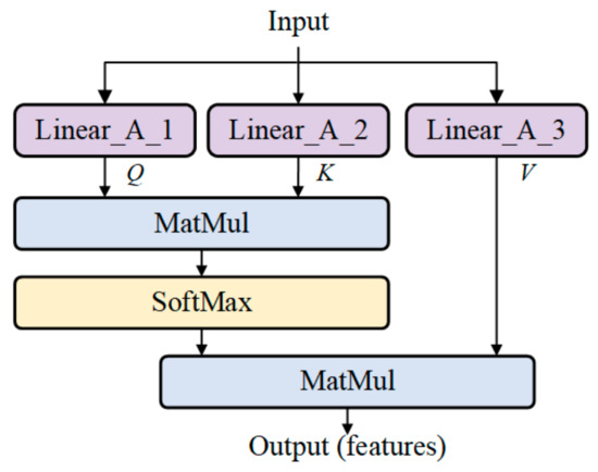
Figure 1.
The structure of Attention Module.
3.2. MSA-Net Model
This paper introduces the proposed Attention module into the model based on the basic structure of MLP. At the same time, to better extract important and potential features, Skip-Connections are used to sum shallow features with mapped features, enabling feature reuse and guiding the synthesis of new features. The network structure is shown in Figure 2.
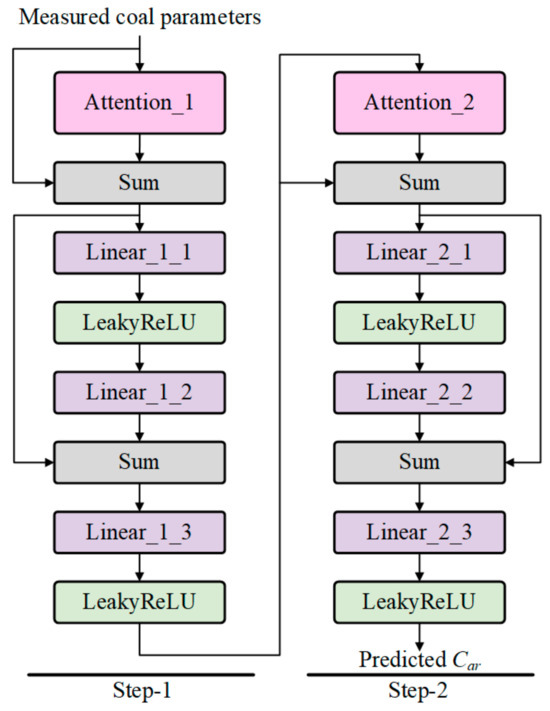
Figure 2.
MSA-Net structure.
MSA-Net consists of two similar structures (Step-1 and Step-2). In Step-1, the input is the measured parameters of coals. The potential features are generated from the Attention module. We utilize 3 linear layers and 2 activation layers for feature integration and mapping, Skip-Connections are added and feature reuse is achieved through Sum operation. The output is the mapped feature. In Step-2, the input is the mapping feature obtained from Step 1, and its structure is similar to that of Step 1. But the output dimension of the last Linear layer is adjusted to 1 for Car prediction. If N-measured parameters are used as input to the model, the corresponding trainable parameters are shown in Table 1. In the experiments, M is set to 128 as the mapping dimension of the hidden layer. Meanwhile, α is set to 0.01 for LeakyReLU.

Table 1.
Parameters of each layer in MSA-Net.
3.3. Loss Function
To ensure the robustness of the model to outliers during training and reduce its sensitivity to outliers, while also ensuring that the gradient gradually decreases as the loss value approaches its minimum, this paper uses the Huber loss Lδ(·) as the loss function for model training. The formula is
where y represents the measured Car, and y′ represents the algorithms or model prediction results. In the experiments, δ is set to 1.0.
4. Training and Predicting Datasets and Evaluation Indicators
4.1. Complete Dataset Production
We collected the measured data of a typical thermal power enterprise from 1 September 2022 to 31 August 2023. This enterprise has two generating units. The daily coal quality analysis and parameter measurements are performed on the coal consumed by both units. Due to shutdowns and routine maintenance, a total of 687 data points were collected. Each data point contains nine parameters: Mt, Mad, Aad, Vad, FCad, Had, St,ad, NCV, and Car. After removing missing and abnormal values, a total of 529 pieces of data were sorted out. We performed maximum and minimum normalization on all measured data in the dataset, and the distribution of normalized Car is shown in Figure 3.
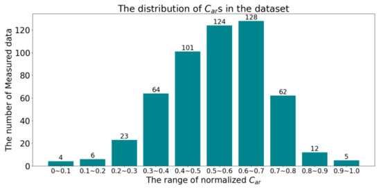
Figure 3.
The distribution of normalized Cars.
4.2. Training and Predicting Datasets Split Methods
In the experiments, training and prediction were performed according to three rules of the dataset created in Section 4.1, according to three rules in the experiment: data partitioning based on stratified sampling, data partitioning based on odd or even months, and data partitioning based on odd or even dates.
4.2.1. Data Partitioning Based on Stratified Sampling
In the experiments of Section 5.2 and Section 5.3, 75% of the data in the dataset was divided into a training set and 25% into a testing set using stratified sampling. The distribution of Cars for this partitioning method is shown in Figure 4.
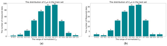
Figure 4.
The distribution of Cars after stratified sampling: (a) The distribution of Cars on the training set; (b) The distribution of Cars on the testing set.
4.2.2. Data Partitioning Based on Odd or Even Months
In the experiments of Section 5.4, we divided each data point into odd and even numbers based on the actual measurement date of each dataset, with a total of 272 odd-month data and 257 even-month data. The distribution of Car for odd and even months is shown in Figure 5.
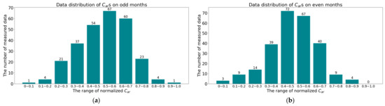
Figure 5.
The distribution of Cars by months: (a) The distribution of Cars on odd months; (b) The distribution of Cars on even months.
4.2.3. Data Partitioning Based on Odd or Even Days
In the experiments of Section 5.5, we further divided the collected 529 data points into odd and even dates, with a total of 223 odd-day data and 306 even-day data. The distribution of Car data for odd days and even numbered days is shown in Figure 6.
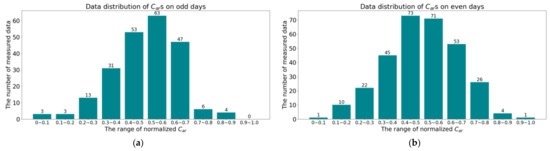
Figure 6.
The distribution of Cars by months: (a) The distribution of Cars on odd days; (b) The distribution of Cars on even days.
4.3. Evaluation Metrics
This paper quantitatively compared the proposed method with existing methods using seven evaluation indicators in the experiment. These evaluation metrics are as follows.
- Mean Absolute Error (MAE)
- 2.
- Root Mean Square Error (RMSE)
- 3.
- Mean Absolute Percentage Error (MAPE)
- 4.
- Coefficient of Determination (R2)
- 5.
- Pearson Correlation Coefficient (PCC)
- 6.
- Concordance Correlation Coefficient (CCC)
- 7.
- Explained Variance (Evar)where δx represents the standard deviation of x, and μx represents the mean of x. The values of MAE, RMSE, and MAPE are all greater than 0, where smaller values indicate better prediction performance. The values of R2, PCC, CCC, and Evar are all between 0 and 1. The closer the value is to 1, the better the model’s prediction performance.
5. Experiments and Analysis
In this section, we compared the performance of MSA-Net with existing models. In addition, we also conducted ablation experiments to analyze the effects of different parts and combinations in MSA-Net. Finally, we conducted application research under different data partitions, providing an effective solution for the practical application of thermal power enterprises when the measured data are incomplete, and further testing the robustness of our trained model.
5.1. Implementation Details
The MSA-Net proposed in this paper is implemented on PyTorch-1.13.0. We conducted model training and testing on NVIDIA GeForce RTX 3070Ti (Graphics Processing Unit produced from NVIDIA Corporation, Santa Clara, CA, USA) with 8 GB of memory. In all experiments, we used the Adam optimizer [31] for model optimization, with β1 = 0.9, β2 = 0.999, and the batch size was set to 16. The model is trained for 240 epochs. The learning rate warm-up strategy [32] was employed during training. The first 40 epochs were the warm-up phase, followed by 200 epochs of learning rate decay. The learning rate lr in each epoch was calculated as
where lrmax is the maximum learning rate in the experiment, which is set to 0.005.
In comparison experiments, we considered two input modes. One refers to the four parameters of the industrial analysis method, including Mad, Aad, Vad, and Qgr,ad. Another type includes all eight parameters. Since the training results of neural network-based methods (such as RNN [33], LSTM [34], MLP [19], and MSA-Net) vary under different parameter initializations, for the same model, we used ten different parameter initialization methods to train the model to convergence using the above parameters. We then statistically evaluated the 10 different prediction results based on the evaluation indicators in Section 4.2. In experiments Section 5.2 and Section 5.4, to verify the effectiveness of the Attention Module, in the MLP, the Attention Module was replaced with a linear layer of size N × N.
All comparative experiments were conducted using two model input methods. Referring to the correlation between measured parameters and elemental carbon content in the industrial analysis method in Section 2, the model input of the first method consists of four parameters: Mad, Aad, Vad, and Qgr,ad. Qgr,ad can be calculated based on NCV, Had, Mt, and Mad. The calculation method is
The model input for the second method includes eight parameters: Mt, Mad, Aad, Vad, FCad, Had, St,ad, and NCV.
5.2. Models Performance Experiments and Analysis
To verify the effectiveness of the proposed model, we compared MSA-Net with existing methods. The comparison results are shown in Table 2. When the input is four parameters, MSA-Net achieved optimal results on all seven metrics. Compared to the GPR model (SOTA), the MSA-Net model achieved lower prediction errors. The MAE decreased by 2.67% (from 4.86 to 4.73) and the RMSE decreased by 2.81% (from 6.77 to 6.58). Compared to the MLP model, the MAE decreased by 6.34% (from 5.05 to 4.73) and the RMSE decreased by 4.78% (from 6.91 to 6.58).
Table 2.
Quantitative evaluation of different models. (RNN, LSTM, MLP, and MSA-Net are the average results).
When the inputs are eight parameters, MSA-Net also achieved the best performance on seven metrics. Compared to the GPR model (SOTA), the MAE decreased by 9.36% (from 5.02 to 4.55) and the RMSE decreased by 10.92% (from 6.96 to 6.20). Compared to the MLP model, the MAE decreased by 6.95% (from 4.89 to 4.55) and RMSE decreased by 6.91% (from 6.66 to 6.20). Due to the Attention module’s focus on important or potential features, when all parameters are used as inputs, MSA-Net can effectively capture the important and potential features, further improving the prediction accuracy. The MAE is reduced by 3.81% (from 4.73 to 4.55), and the RMSE is reduced by 5.78% (from 6.58 to 6.20).
Due to the differences in training results of neural network models under different parameter initializations, we also counted the prediction results under different parameter initializations. After sorting out the prediction results of some samples, a box plot is drawn as shown in Figure 7. When the inputs are four or eight parameters, the uncertainty of MSA-Net prediction results is significantly smaller than RNN, LSTM, and MLP models, and the median is also closer to the measured true value. We further summarized the mean and standard deviation of the prediction errors on the test set, as shown in Table 3. When given four input parameters, MSA-Net achieved the best performance on all seven evaluation metrics in terms of both the mean and standard deviation. When given eight input parameters, MSA-Net achieved the best performance on all seven evaluation metrics in terms of the mean. In addition, it achieved the lowest standard deviation on three metrics. Overall, MSA-Net not only achieves good prediction accuracy but also has stable prediction results under different parameter initializations after training.
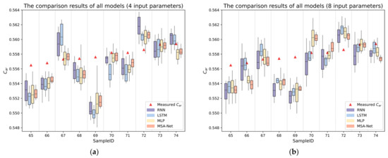
Figure 7.
Visual comparison of partial prediction results in the test set: (a) The comparison results of different models (input four parameters); (b) The comparison results of different models (input eight input parameters).
Table 3.
Quantitative evaluation of model accuracy and stability.
5.3. Ablation Analysis
To verify the effectiveness of the proposed modules, we conducted ablation experiments as shown in Table 4. By adopting Huber loss on the MLP (Model A), the MAE can be reduced by 1.78% (from 5.05 to 4.96). By adding one Attention module (Model B), the MAE is reduced by 1.01% (from 4.96 to 4.91). With two Attention modules (Model C), the MAE is further reduced by 1.81% (from 4.96 to 4.87). However, when increasing the number of Attention modules to three (Model D), the prediction accuracy of the model has significantly decreased. By incorporating Skip-Connections on the basis of two Attention modules, the proposed MSA-Net can further reduce the MAE by 2.87% (from 4.87 to 4.73). When the number of input parameters is increased from four to eight, the MAE is reduced by 3.81% (from 4.73 to 4.55).
Table 4.
Ablation analysis results of each module.
5.4. Model Testing Experiments on Dividing Datasets on Odd and Even Months
We quantitatively compared MSA-Net with RNN, LSTM, and MLP on seven evaluation metrics, and presented the mean and standard deviation of each metric under 10 different parameter initialization methods. We conducted this part of the experiment in two ways. The first method was to train the model using odd-month data and make predictions on even-month data. The quantitative comparison results are shown in Table 5. The second method is to use even-month data for model training and predict odd-month data. The quantitative comparison results are shown in Table 6.
Table 5.
The odd-month data are used for model training, and the even-month data are used for quantitative evaluation of prediction.
Table 6.
The even-month data are used for model training, and the odd-month data are used for quantitative evaluation of prediction.
By comparing the prediction errors of different models, in Table 5, when the inputs are four parameters, the MSA-Net model reduces RMSE by 12.97% (from 7.40 to 6.44) compared to the RNN model. Compared with the LSTM model, RMSE decreases by 15.15% (from 7.59 to 6.44), and RMSE decreases by 8.00% (from 7.00 to 6.44) compared to the MLP model. The MSA-Net model reduces RMSE by 3.88% (from 6.70 to 6.44) compared to the Transformer model. When the inputs are eight parameters, taking the RMSE index as an example, MSA-Net decreased by 14.55% (from 7.49 to 6.40) compared to RNN, 18.26% (from 7.83 to 6.40) compared to LSTM, 12.81% (from 7.34 to 6.40) compared to MLP, and 2.44% (from 6.56 to 6.40) compared to Transformer. When the number of input parameters increased from four to eight, the MAE of the MSA-Net model decreased by 1.87% (from 4.81 to 4.72). In Table 6, when inputting four parameters, the MSA-Net model reduces RMSE by 11.19% (from 6.97 to 6.19) compared to the RNN model, and reduces RMSE by 11.32% (from 6.98 to 6.19) compared to the MLP model. The MSA-Net model reduces RMSE by 7.06% (from 6.66 to 6.19) compared to the Transformer model. When the number of input parameters increased from four to eight, the accuracy of the MSA-Net model slightly decreased, and the MAE increased by 0.70% (from 4.31 to 4.34).
By comparing the predictive stability of different models, in Table 5 and Table 6, when the inputs are four or eight parameters, MSA-Net has the smallest standard deviation on seven indicators compared to RNN, LSTM, MLP, and Transformer, indicating that MSA-Net can predict more stably under different parameter initialization conditions.
In summary, for the thermal power enterprises, within a one-year statistical period, they can measure the elemental carbon in the first nine months according to the requirements and use these measured data for training the MSA-Net model. In the last three months, they only need to measure the Mad, Aad, Vad, and Qgr,ad to predict the Cad using the trained MSA-Net model. After that, the measured Mt can be used to convert Cad to Car.
5.5. Model Testing Experiments on Dividing Datasets on Odd and Even Days
We conducted this part of the experiment in two ways. The first method was to train the model using odd-day data and make predictions on even-day data. The quantitative comparison results are shown in Table 7. The second method is to use even-day data for model training and predict odd-day data. The quantitative comparison results are shown in Table 8. When the inputs are eight parameters, MSA-Net has a 20.0% decrease in RMSE compared to MLP (from 7.45 to 5.96). The MSA-Net model reduces RMSE by 7.74% (from 6.46 to 5.96) compared to the Transformer model. In the second method, when the inputs are eight parameters, MSA-Net has an 8.66% decrease in RMSE compared to MLP (from 7.04 to 6.43). The MSA-Net model reduces RMSE by 7.35% (from 6.94 to 6.43) compared to the Transformer model. In addition, MSA-Net has the smallest standard deviation on seven indicators under each partition and different input conditions, indicating good predictive stability. Due to the inconsistent distribution of single- and double-day data, as well as the relatively small proportion of training data to test data, the model learning difficulty is high. Among all comparison models, MSA-Net still achieved the best prediction accuracy, with MAPE of only 0.76% (input four parameters) and 0.87% (input eight parameters).
Table 7.
The odd-day data are used for model training, and the even-day data are used for quantitative evaluation of prediction.
Table 8.
The even-day data are used for model training, and the odd-day data are used for quantitative evaluation of prediction.
In summary, within a one-year statistical period, thermal power enterprises can conduct complete data measurements of elemental carbon on odd (even) days and use these measured data for training the MSA-Net model. On even (odd) days, they can measure the Mt, Mad, Aad, Vad, FCad, Had, St,ad, and NCV. With these parameters, the trained MSA-Net can predict the Car.
6. Discussion
In Section 5.1, we introduced the four commonly used parameters in proximate analysis. When only Mad, Aad, Vad, and Qgr,ad are used, it contains a total of six parameters including Mad, Aad, Vad, FCad, NCV, and Had. This parameter selection method completely ignores the effect of St,ad (from ultimate analysis) on Car calculation. If we further increase the parameters St,ad, MSA-Net will have a further improvement compared to inputting four parameters as shown in Table 9. However, due to the inherent inclusion of other parameters, effective decoupling is not possible. Therefore, in most cases, MSA-Net with eight inputs can achieve the highest accuracy.
Table 9.
The impact of different input parameters on MSA-Net.
7. Conclusions
Car is an important parameter for carbon accounting in thermal power enterprises. However, in actual production processes, due to equipment maintenance, repairs, or damage, measurement data may be missing. Using default values will increase the compliance costs of the enterprises. Therefore, it is of great significance to use reliable prediction models to accurately predict Car when measurement data are missing, in order to ensure the accuracy of carbon accounting and protect the interests of the enterprise. Based on existing research, this paper first analyzes the parameters related to Car. Secondly, these parameters are used as input to propose a carbon content prediction model based on the attention mechanism called MSA-Net. The construction process and details of the Attention module are introduced in detail. Then, the complete measured data are collected from thermal power enterprises, and after data preprocessing, a Car prediction dataset is constructed for model training and testing. Subsequently, the effectiveness and reliability of MSA-Net are verified by comparing it with existing methods on the constructed dataset. Finally, two solutions are proposed to reduce the frequency of measurements for thermal power enterprises, thereby reducing their detection costs.
Author Contributions
Conceptualization, Y.W. and X.X.; methodology, Y.W.; software, Y.W. and F.C.; validation, Z.L. and X.X.; formal analysis, X.X.; investigation, Z.L.; resources, X.X.; data curation, Y.W.; writing—original draft preparation, Y.W.; writing—review and editing, Y.W. and X.X.; visualization, F.C.; supervision, Z.L.; project administration, Y.W. and X.X.; funding acquisition, X.X. All authors have read and agreed to the published version of the manuscript.
Funding
This research was funded by the China National Key R&D Program, grant number 2021YFF0600100.
Institutional Review Board Statement
Not applicable.
Informed Consent Statement
Not applicable.
Data Availability Statement
The original contributions presented in the study are included in the article, further inquiries can be directed to the corresponding author/s.
Conflicts of Interest
The authors declare no conflicts of interest.
References
- Brown, H. Reducing the impact of climate change. Bull. World Health Organ. 2022, 85, 824–825. [Google Scholar]
- Li, J.; Wang, P.; Ma, S. The impact of different transportation infrastructures on urban carbon emissions: Evidence from China. Energy 2024, 295, 131041. [Google Scholar] [CrossRef]
- Wu, X.; Liu, P.; Yang, L.; Shi, Z.; Lao, Y. Impact of three carbon emission reduction policies on carbon verification behavior: An analysis based on evolutionary game theory. Energy 2024, 295, 130926. [Google Scholar] [CrossRef]
- Qiao, Q.; Eskandari, H.; Saadatmand, H.; Sahraei, M.A. An interpretable multi-stage forecasting framework for energy consumption and CO2 emissions for the transportation sector. Energy 2024, 286, 129499. [Google Scholar] [CrossRef]
- Ditl, P.; Šulc, R. Calculations of CO2 emission and combustion efficiency for various fuels. Energy 2024, 290, 130044. [Google Scholar] [CrossRef]
- International Energy Agency (IEA). CO2 Emissions in 2022. 2022. Available online: https://www.iea.org/reports/co2-emissions-in-2022 (accessed on 15 June 2024).
- Zhang, S.; Zhao, T.; Xie, B.-C.; Gao, J. What drives the GHG emission changes of the electric power industry in China? An empirical analysis using the logarithmic mean divisia index method. Carbon Manag. 2017, 8, 363–377. [Google Scholar] [CrossRef]
- Wang, Y.; Song, J.; Yang, W.; Dong, L.; Duan, H. Unveiling the driving mechanism of air pollutant emissions from thermal power generation in China: A provincial-level spatiotemporal analysis. Resour. Conserv. Recycl. 2019, 151, 104447. [Google Scholar] [CrossRef]
- GB/T 32151.1-2015; Requirements of the Greenhouse Gas Emission Accounting and Reporting—Part 1: Power Generation Enterprise. Standardization Administration of the People’s Republic of China: Beijing, China, 2015.
- Ministry of Ecology and Environment of the People’s Republic of China. Notice on Issuing the Guidelines for Accounting and Reporting of Green-House Gas Emissions by Enterprises—Power Generation Facilities and the Technical Guidelines for Verification of Greenhouse Gas Emissions by Enterprises Power Generation Facilities. 2022. Available online: https://www.mee.gov.cn/xxgk2018/xxgk/xxgk06/202212/t20221221_1008430.html (accessed on 15 June 2024).
- Ministry of Ecology and Environment of the People’s Republic of China. Notice on the Key Tasks of Efficient Coordination of Epidemic Prevention and Control and Economic and Social Development Adjustment for 2022 Enterprise Greenhouse Gas Emission Report Management. 2022. Available online: https://www.gov.cn/zhengce/zhengceku/2022-06/12/content_5695325.htm (accessed on 15 June 2024).
- Zhang, F.; Li, H.; Xu, Z.; Chen, W. A novel abrm model for predicting coal moisture content. J. Intell. Robot. Syst. 2022, 104, 30. [Google Scholar] [CrossRef] [PubMed]
- Liu, Y.; Zhang, H.; Zhang, X.; Qing, S.; Zhang, A.; Yang, S. Optimization of Combustion Characteristics of Blended Coals Based on TOPSIS Method. Complexity 2018, 2018, 4057983. [Google Scholar] [CrossRef]
- Shu, P.; Zhang, Y.; Deng, J.; Zhang, Y.; Duan, Z.; Li, L. Study on the effect of mixed particle size on coal heat release characteristics. Int. J. Coal Prep. Util. 2023, 43, 831–846. [Google Scholar] [CrossRef]
- Deng, S.; Hu, Y.; Chen, D.; Ma, Z.; Li, H. Integrated petrophysical log evaluation for coalbed methane in the hancheng area, China. J. Geophys. Eng. 2013, 10, 035009. [Google Scholar] [CrossRef]
- Guan, C.; Wu, T.; Chen, J.; Li, M. Detection of carbon content from pulverized coal using libs coupled with DSC-PLS method. Chemosensors 2022, 10, 490. [Google Scholar] [CrossRef]
- Jo, J.; Lee, D.-G.; Kim, J.; Lee, B.-H.; Jeon, C.-H. Improved ann-based approach using relative impact for the prediction of thermal coal elemental composition using proximate analysis. ACS Omega 2022, 7, 29734–29746. [Google Scholar] [CrossRef] [PubMed]
- Ceylan, Z.; Sungur, B. Estimation of coal elemental composition from proximate analysis using machine learning techniques. Energy Sources Part A Recov. Util. Environ. Eff. 2020, 42, 2576–2592. [Google Scholar] [CrossRef]
- Yin, L.; Liu, G.; Zhou, J.; Liao, Y.; Ma, X. A calculation method for CO2 emission in utility boilers based on bp neural network and carbon balance. Energy Procedia 2017, 105, 3173–3178. [Google Scholar] [CrossRef]
- Ashish, V.; Noam, S.; Niki, P.; Jakob, U.; Llion, J.; Aidan, N.G.; Lukas, K.; Illia, P. Attention is all you need. In Proceedings of the 31st Conference on Neural Information Processing Systems (NIPS 2017), Long Beach, CA, USA, 4–9 December 2017; Curran Associates Inc.: Red Hook, NY, USA, 2017. [Google Scholar]
- Liu, F.; Ren, X.; Zhang, Z.; Sun, X.; Zou, Y. Rethinking skip connection with layer normalization in transformers and resnets. arXiv 2021, arXiv:2105.07205. [Google Scholar]
- Zhu, D. Application of carbon ultimate analysis into greenhouse gas emissions accounting for coal-fired power plants. Power Gener. Technol. 2018, 39, 363–366. [Google Scholar]
- GB/T 30732-2014; Proximate Analysis of Coal—Instrumental Method. General Administration of Quality Supervision, Inspection and Quarantine of the People’s Republic of China. Standardization Administration of the People’s Republic of China: Beijing, China, 2014.
- GB/T 31391-2015; Ultimate Analysis of Coal. General Administration of Quality Supervision, Inspection and Quarantine of the People’s Republic of China. Standardization Administration of the People’s Republic of China: Beijing, China, 2015.
- GB/T 213-2008; Determination of Calorific Value of Coal. General Administration of Quality Supervision, Inspection and Quarantine of the People’s Republic of China. Standardization Administration of the People’s Republic of China: Beijing, China, 2008.
- GB/T 211-2017; Determination of Moisture in Coal. General Administration of Quality Supervision, Inspection and Quarantine of the People’s Republic of China. Standardization Administration of the People’s Republic of China: Beijing, China, 2017.
- GB/T 212-2008; Proximate Analysis of Coal. General Administration of Quality Supervision, Inspection and Quarantine of the People’s Republic of China. Standardization Administration of the People’s Republic of China: Beijing, China, 2008.
- GB/T 214-2007; Determination of Total Sulfur in Coal. General Administration of Quality Supervision, Inspection and Quarantine of the People’s Republic of China. Standardization Administration of the People’s Republic of China: Beijing, China, 2007.
- GB/T 476-2008; Determination of Carbon and Hydrogen in Coal. General Administration of Quality Supervision, Inspection and Quarantine of the People’s Republic of China. Standardization Administration of the People’s Republic of China: Beijing, China, 2008.
- Liu, J.; Sun, M.; Zhang, W.; Xie, G.; Jing, Y.; Li, X.; Shi, Z. Dae-ner: Dual-channel attention enhancement for chinese named entity recognition. Comput. Speech Lang. 2024, 85, 101581. [Google Scholar] [CrossRef]
- Kingma, D.P.; Ba, J. Adam: A method for stochastic optimization. arXiv 2014, arXiv:1412.6980. [Google Scholar]
- He, K.; Zhang, X.; Ren, S.; Sun, J. Deep residual learning for image recognition. In Proceedings of the 2016 IEEE Conference on Computer Vision and Pattern Recognition (CVPR), Las Vegas, NV, USA, 27–30 June 2016; pp. 770–778. [Google Scholar]
- Lipton, Z.C. A critical review of recurrent neural networks for sequence learning. arXiv 2015, arXiv:1506.00019. [Google Scholar]
- Mulás-Tejeda, E.; Gómez-Espinosa, A.; Escobedo Cabello, J.A.; Cantoral-Ceballos, J.A.; Molina-Leal, A. Implementation of a Long Short-Term Memory Neural Network-Based Algorithm for Dynamic Obstacle Avoidance. Sensors 2024, 24, 3004. [Google Scholar] [CrossRef] [PubMed]
- Du, Q.; Wang, Z.; Huang, P.; Zhai, Y.; Yang, X.; Ma, S. Remote Sensing Monitoring of Grassland Locust Density Based on Machine Learning. Sensors 2024, 24, 3121. [Google Scholar] [CrossRef] [PubMed]
- Yan, Z.; Qin, Z.; Fan, J.; Huang, Y.; Wang, Y.; Zhang, J.; Zhang, L.; Cao, Y. Gas Outburst Warning Method in Driving Faces: Enhanced Methodology through Optuna Optimization, Adaptive Normalization, and Transformer Framework. Sensors 2024, 24, 3150. [Google Scholar] [CrossRef] [PubMed]
- Xiao, P.; Chen, D. Photothermal Radiometry Data Analysis by Using Machine Learning. Sensors 2024, 24, 3015. [Google Scholar] [CrossRef] [PubMed]


Disclaimer/Publisher’s Note: The statements, opinions and data contained in all publications are solely those of the individual author(s) and contributor(s) and not of MDPI and/or the editor(s). MDPI and/or the editor(s) disclaim responsibility for any injury to people or property resulting from any ideas, methods, instructions or products referred to in the content. |
© 2024 by the authors. Licensee MDPI, Basel, Switzerland. This article is an open access article distributed under the terms and conditions of the Creative Commons Attribution (CC BY) license (https://creativecommons.org/licenses/by/4.0/).