
Compact Chromatic Confocal Lens with Large Measurement Range

 , and
, and
Abstract
1. Introduction
2. Design of Dispersive Objective Lens
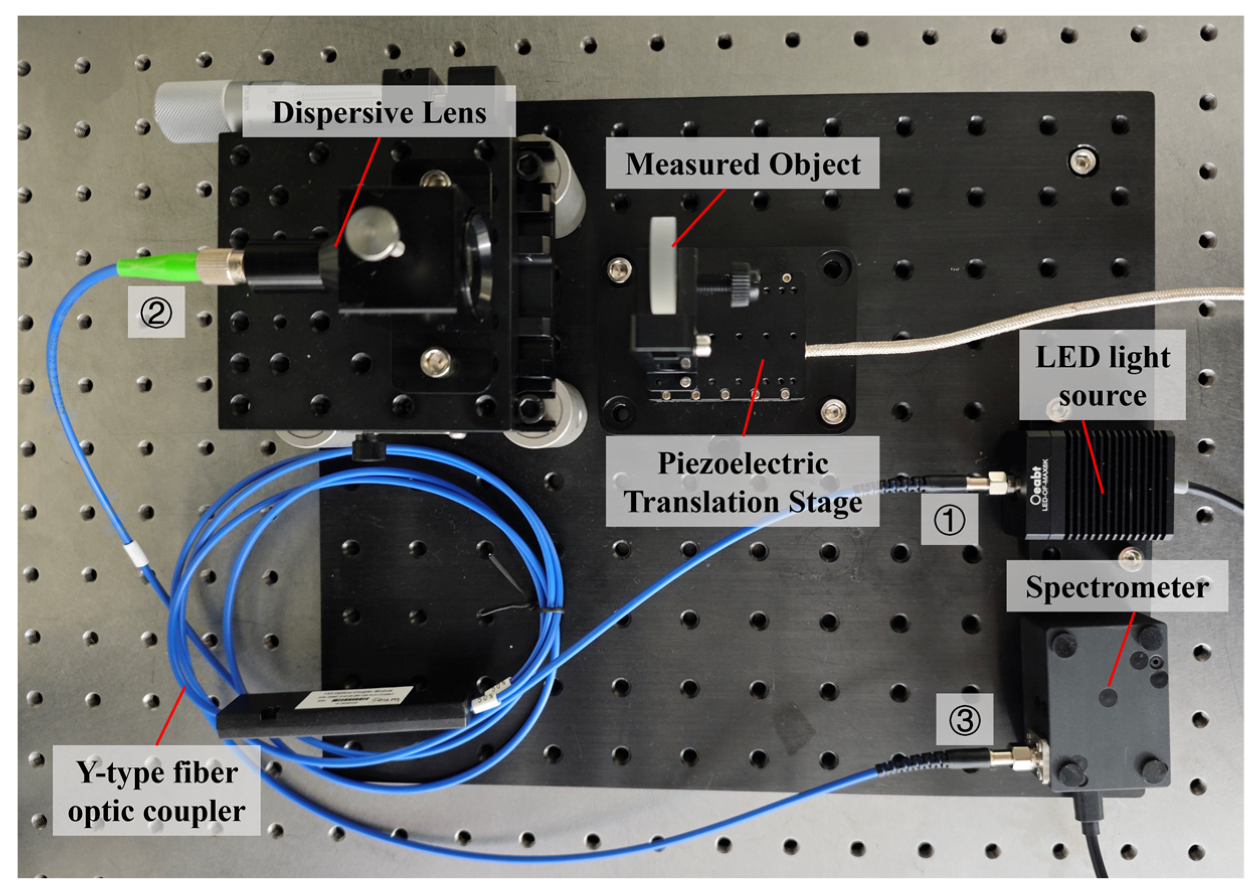
2.1. Spectral Confocal Measurement System Construction
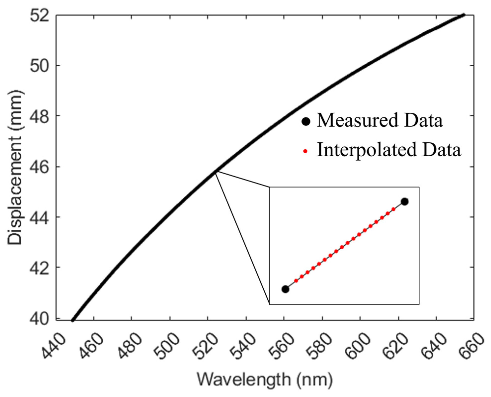
2.2. Design of Dispersive Objective Lens
3. Results
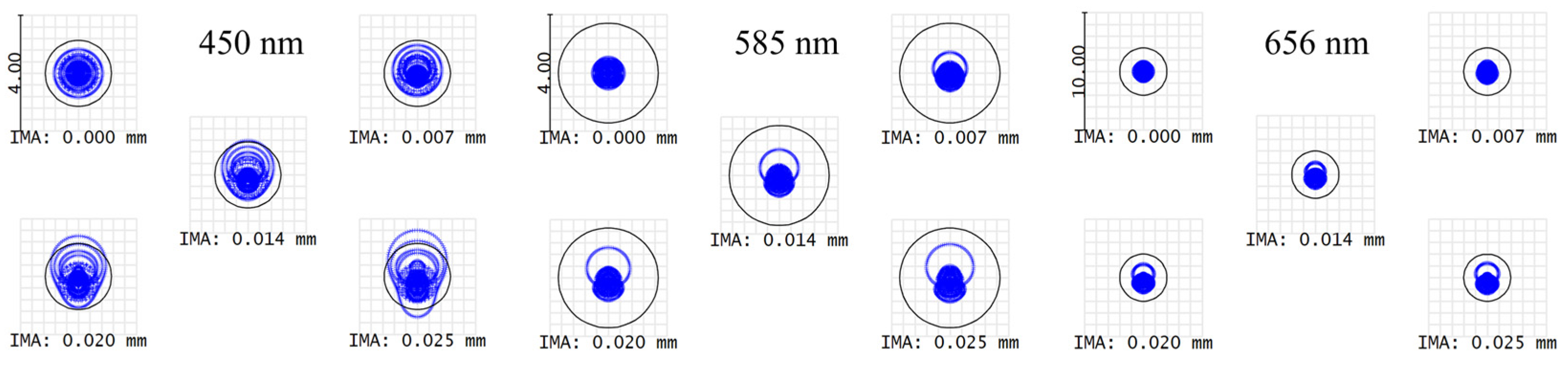
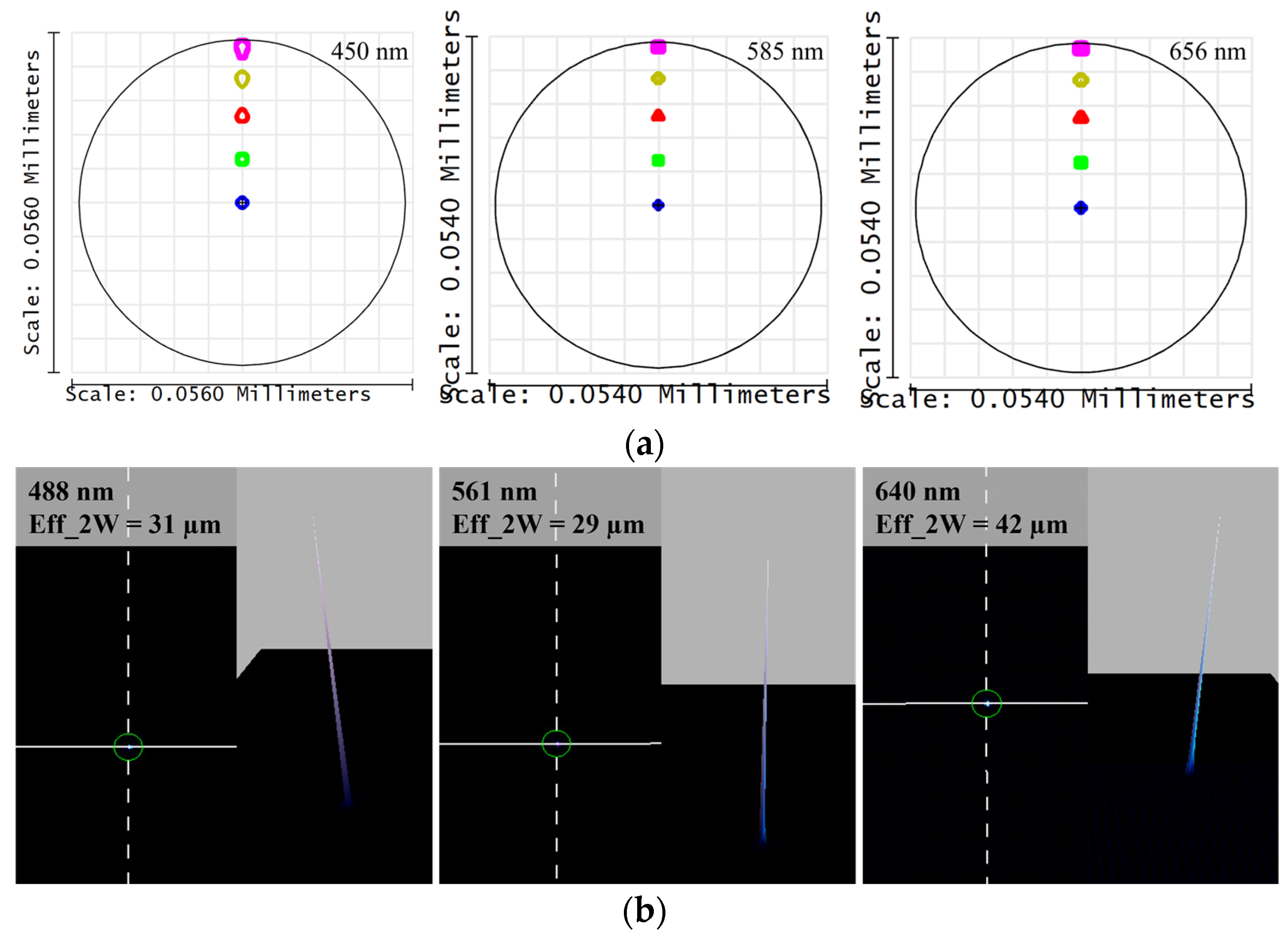
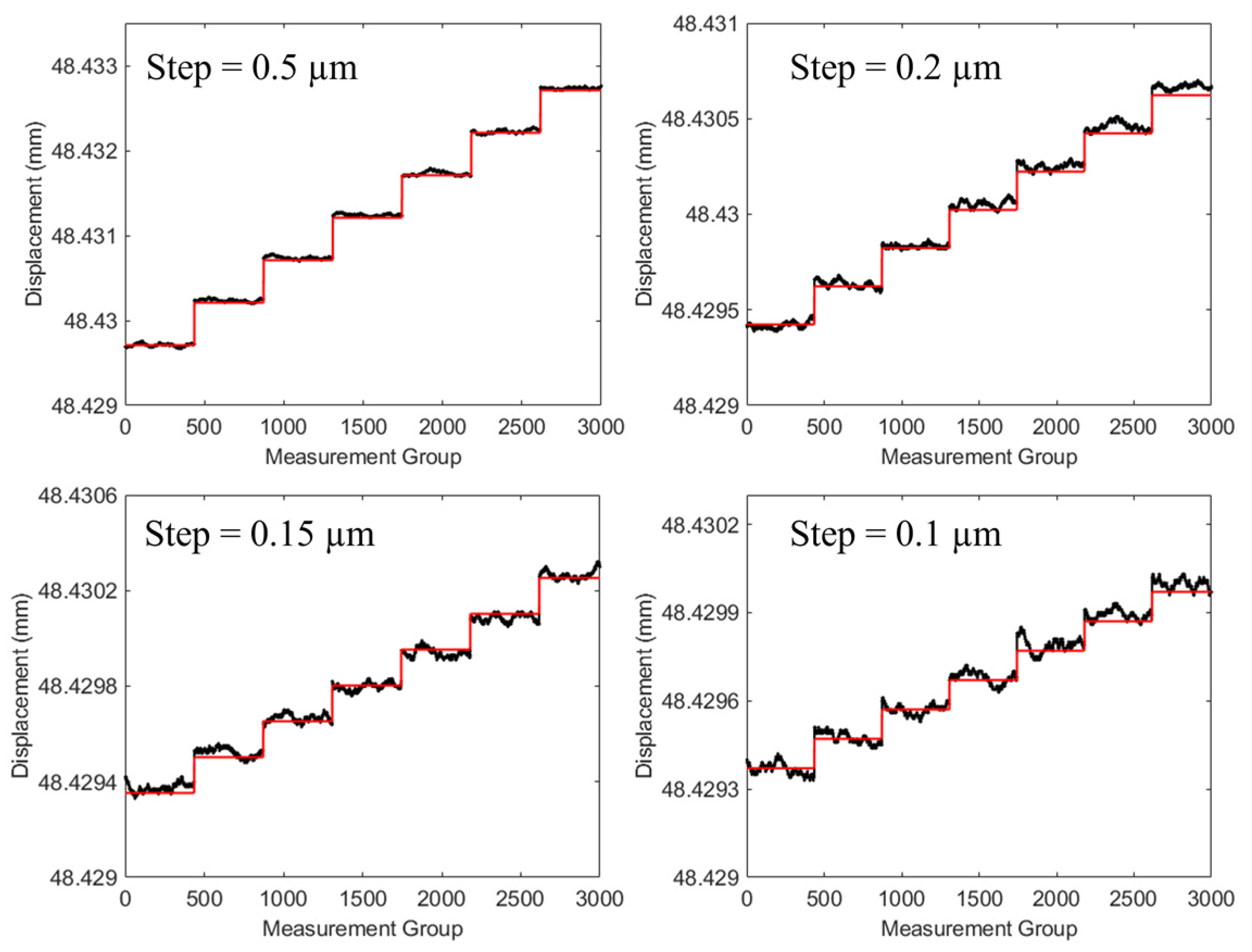
3.1. Resolution
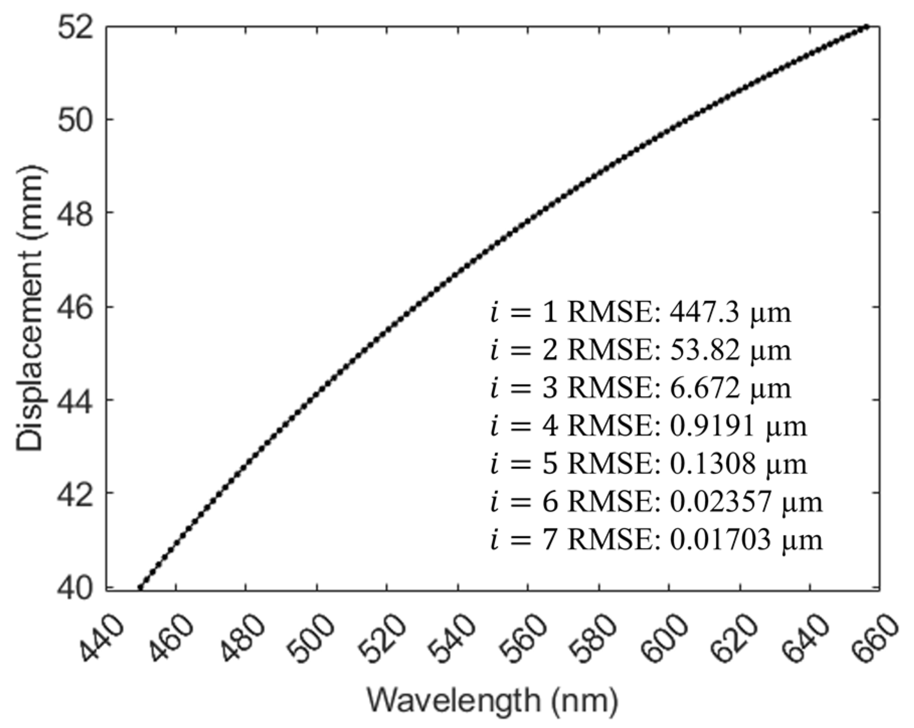
3.2. Maximum Linear Error
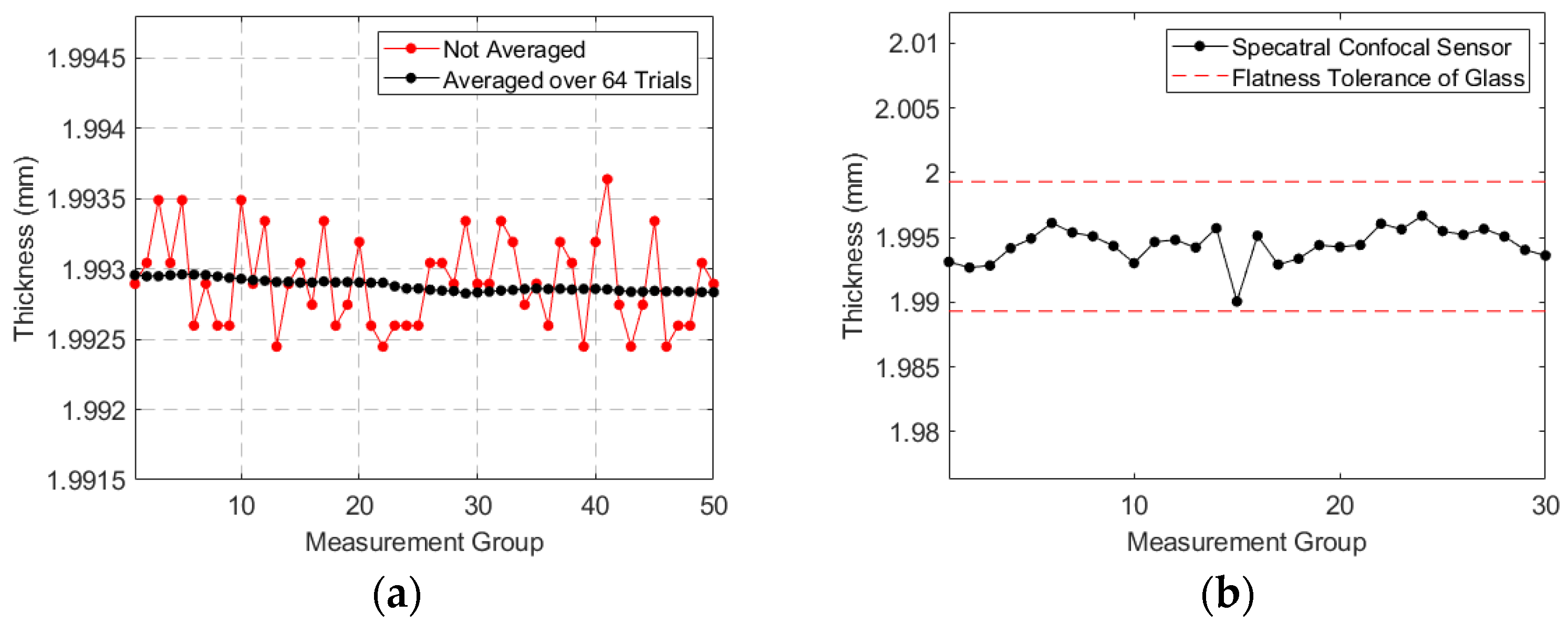
3.3. Thickness Measurement
4. Conclusions
Author Contributions
Funding
Data Availability Statement
Conflicts of Interest
References
- Kim, S.-W.; Kim, G.-H. Thickness-Profile Measurement of Transparent Thin-Film Layers by White-Light Scanning Interferometry. Appl. Opt. 1999, 38, 5968–5973. [Google Scholar] [CrossRef] [PubMed]
- Schmit, J.; Olszak, A. High-Precision Shape Measurement by White-Light Interferometry with Real-Time Scanner Error Correction. Appl. Opt. 2002, 41, 5943–5950. [Google Scholar] [CrossRef] [PubMed]
- Yang, S.; Zhang, G. A Review of Interferometry for Geometric Measurement. Meas. Sci. Technol. 2018, 29, 102001. [Google Scholar] [CrossRef]
- Pan, W.; Zhang, D.; Liang, C.; Ma, C.; Shu, X.; Che, S.; Hu, H. A High-Precision Laser Displacement Measurement System. In Proceedings of the AOPC 2021: Optical Sensing and Imaging Technology; SPIE: Bellingham, WA, USA, 2021; Volume 12065, pp. 554–559. [Google Scholar]
- Nalimov, A.; Stafeev, S.; Kotlyar, V.; Kozlova, E. Optical Sensor Methodology for Measuring Shift, Thickness, Refractive Index and Tilt Angle of Thin Films. Photonics 2023, 10, 690. [Google Scholar] [CrossRef]
- Miks, A.; Novak, J.; Novak, P. Analysis of Method for Measuring Thickness of Plane-Parallel Plates and Lenses Using Chromatic Confocal Sensor. Appl. Opt. 2010, 49, 3259–3264. [Google Scholar] [CrossRef] [PubMed]
- Yu, Q.; Zhang, K.; Cui, C.; Zhou, R.; Cheng, F.; Ye, R.; Zhang, Y. Method of Thickness Measurement for Transparent Specimens with Chromatic Confocal Microscopy. Appl. Opt. 2018, 57, 9722–9728. [Google Scholar] [CrossRef] [PubMed]
- Zhou, R.; Shen, D.; Huang, P.; Kong, L.; Zhu, Z. Chromatic Confocal Sensor-Based Sub-Aperture Scanning and Stitching for the Measurement of Microstructured Optical Surfaces. Opt. Express 2021, 29, 33512–33526. [Google Scholar] [CrossRef] [PubMed]
- Wertjanz, D.; Kern, T.; Csencsics, E.; Stadler, G.; Schitter, G. Compact Scanning Confocal Chromatic Sensor Enabling Precision 3-D Measurements. Appl. Opt. 2021, 60, 7511–7517. [Google Scholar] [CrossRef] [PubMed]
- Chen, H.-R.; Chen, L.-C. Full-Field Chromatic Confocal Microscopy for Surface Profilometry with Sub-Micrometer Accuracy. Opt. Lasers Eng. 2023, 161, 107384. [Google Scholar] [CrossRef]
- Molesini, G.; Pedrini, G.; Poggi, P.; Quercioli, F. Focus-Wavelength Encoded Optical Profilometer. Opt. Commun. 1984, 49, 229–233. [Google Scholar] [CrossRef]
- Bai, J.; Li, X.; Wang, X.; Zhou, Q.; Ni, K. Chromatic Confocal Displacement Sensor with Optimized Dispersion Probe and Modified Centroid Peak Extraction Algorithm. Sensors 2019, 19, 3592. [Google Scholar] [CrossRef] [PubMed]
- Jiang, W.; Zeng, A.; Huang, H. Design of Linear Hyperchromatic Lens in Chromatic Focal Displacement Sensor. In Proceedings of the AOPC 2020: Optics Ultra Precision Manufacturing and Testing; Zhang, D., Kong, L., Luo, X., Eds.; SPIE: Beijing, China, 2020; p. 6. [Google Scholar]
- Xie, Z.; Liu, R.; Zou, K.; Zhou, J. Design of Dispersive Objective Lens of Spectral Confocal Displacement Sensor. In Proceedings of the 2021 IEEE Asia-Pacific Conference on Image Processing, Electronics and Computers (IPEC), Dalian, China, 14–16 April 2021; pp. 533–535. [Google Scholar]
- Li, C.; Li, K.; Liu, J.; Lv, Z.; Li, G.; Li, D. Design of a Confocal Dispersion Objective Lens Based on the GRIN Lens. Opt. Express 2022, 30, 44290. [Google Scholar] [CrossRef] [PubMed]
- Liu, T.; Wang, J.; Liu, Q.; Hu, J.; Wang, Z.; Wan, C.; Yang, S. Chromatic Confocal Measurement Method Using a Phase Fresnel Zone Plate. Opt. Express 2022, 30, 2390. [Google Scholar] [CrossRef] [PubMed]
- Bai, J.; Li, X.; Zhou, Q.; Ni, K.; Wang, X. Improved Chromatic Confocal Displacement-Sensor Based on a Spatial-Bandpass-Filter and an X-Shaped Fiber-Coupler. Opt. Express 2019, 27, 10961. [Google Scholar] [CrossRef] [PubMed]
- Liu, C.; Lu, G.; Liu, C.; Li, D. Compact Chromatic Confocal Sensor for Displacement and Thickness Measurements. Meas. Sci. Technol. 2023, 34, 055104. [Google Scholar] [CrossRef]
- Zakrzewski, A.; Ćwikła, M.; Koruba, P.; Jurewicz, P.; Reiner, J. Design of a Chromatic Confocal Displacement Sensor Integrated with an Optical Laser Head. Appl. Opt. 2020, 59, 9108–9117. [Google Scholar] [CrossRef] [PubMed]
- Novak, J.; Miks, A. Hyperchromats with Linear Dependence of Longitudinal Chromatic Aberration on Wavelength. Optik 2005, 116, 165–168. [Google Scholar] [CrossRef]
- Browne, M.A.; Akinyemi, O.; Boyde, A. Confocal Surface Profiling Utilizing Chromatic Aberration. Scanning 1992, 14, 145–153. [Google Scholar] [CrossRef]
- Hillenbrand, M.; Weiss, R.; Endrödy, C.; Grewe, A.; Hoffmann, M.; Sinzinger, S. Chromatic Confocal Matrix Sensor with Actuated Pinhole Arrays. Appl. Opt. 2015, 54, 4927–4936. [Google Scholar] [CrossRef] [PubMed]


| Equipment | Specification |
|---|---|
| Y-type fiber optic coupler | Core diameter: 50 μm Splitting ratio: 1:1 NA: 0.22 |
| LED light source | LED-OF-MAX6K |
| Spectrometer | Flexible 4000 Resolution: 2.3 nm |
| Piezoelectric translation stage | CoreMorrow N5630E-B1 |
| Parameter | Value |
|---|---|
| Working wavelength | 450–656 nm |
| Working distance | 46 ± 6 mm |
| Axial dispersion | 12 mm |
| Object-side NA | 0.22 |
| Image-side NA’ | 0.198–0.24 |
| Surface | Radius | Thickness | Clear Semi-Dia |
|---|---|---|---|
| OBJECT | Infinity | 3 | 0.027 |
| 1 | Infinity | 4.9 | 0.677 |
| 2 | 5.1 | 4 | 3.5 |
| 3 | Infinity | 7.26 | 3.5 |
| 4 | −5.7 | 4 | 2.076 |
| 5 | 9.8 | 10.4 | 2.877 |
| 6 | −30 | 5 | 8.278 |
| 7 | −17.2 | 0 | 11.5 |
| 8 | 34.7 | 5 | 11.5 |
| 9 | −63.85 | 5.5 | 11.5 |
| 10 | −15.8 | 5 | 9.857 |
| 11 | −49.4 | 4 | 11.5 |
| 12 | −21.4 | 40 | 11.5 |
| IMAGE | Infinity | 0.027 |
| Tolerance Terms | Allocation Value |
|---|---|
| Thickness | 0.01 mm |
| Surface tilt | 0.3‘ |
| Component tilt | 0.3‘ |
| Surface eccentricity | 0.003 mm |
| S + A irregularity | 0.1 |
| Component eccentricity | 0.01 |
| Refractive index | 0.0003 |
| Aberration | 0.03% |
| Wavelength | Radius of Airy Spot | 90% Probability RMS in Monte Carlo Analysis |
|---|---|---|
| 450 nm | 1.143 μm | 3.30110 μm |
| 585 nm | 1.714 μm | 4.11116 μm |
| 656 nm | 2.003 μm | 4.26328 μm |
Disclaimer/Publisher’s Note: The statements, opinions and data contained in all publications are solely those of the individual author(s) and contributor(s) and not of MDPI and/or the editor(s). MDPI and/or the editor(s) disclaim responsibility for any injury to people or property resulting from any ideas, methods, instructions or products referred to in the content. |
© 2024 by the authors. Licensee MDPI, Basel, Switzerland. This article is an open access article distributed under the terms and conditions of the Creative Commons Attribution (CC BY) license (https://creativecommons.org/licenses/by/4.0/).
Share and Cite
He, N.; Hu, H.; Cui, Z.; Xu, X.; Zhou, D.; Chen, Y.; Gong, P.; Chen, Y.; Kuang, C. Compact Chromatic Confocal Lens with Large Measurement Range. Sensors 2024, 24, 5122. https://doi.org/10.3390/s24165122
He N, Hu H, Cui Z, Xu X, Zhou D, Chen Y, Gong P, Chen Y, Kuang C. Compact Chromatic Confocal Lens with Large Measurement Range. Sensors. 2024; 24(16):5122. https://doi.org/10.3390/s24165122
Chicago/Turabian StyleHe, Ning, Huiqin Hu, Zhiying Cui, Xinjun Xu, Dakai Zhou, Yunbo Chen, Puyin Gong, Youhua Chen, and Cuifang Kuang. 2024. "Compact Chromatic Confocal Lens with Large Measurement Range" Sensors 24, no. 16: 5122. https://doi.org/10.3390/s24165122
APA StyleHe, N., Hu, H., Cui, Z., Xu, X., Zhou, D., Chen, Y., Gong, P., Chen, Y., & Kuang, C. (2024). Compact Chromatic Confocal Lens with Large Measurement Range. Sensors, 24(16), 5122. https://doi.org/10.3390/s24165122