
From Near-Sensor to In-Sensor: A State-of-the-Art Review of Embedded AI Vision Systems

Abstract
:1. Introduction
- Sensors generate massive amounts of data, which can lead to processing and communication bottlenecks in cloud computing.
- Real-time processing requirements often exceed the latency capabilities of cloud computing.
- Computation and communication with or in the cloud, and specifically access to the data generated by computations, require high energy consumption [22].
1.1. Embedded AI Vision Systems Categories
1.2. Design Space: From Near-Sensor to In-Sensor
1.2.1. Near-Sensor AI Vision Systems
1.2.2. In-Sensor AI Vision Systems
2. Metrics and Characteristics
2.1. Image Acquisition Characteristics
2.1.1. Capture Resolution
2.1.2. Processing Resolution
2.2. Pixel-Level Processing
2.2.1. Image Signal Processor
2.2.2. Pre-Processing
2.3. Bandwidth and Interconnect
2.3.1. Analog-to-Digital Bandwidth
2.3.2. Digital Interconnect Bandwidth
2.4. Memory Resources
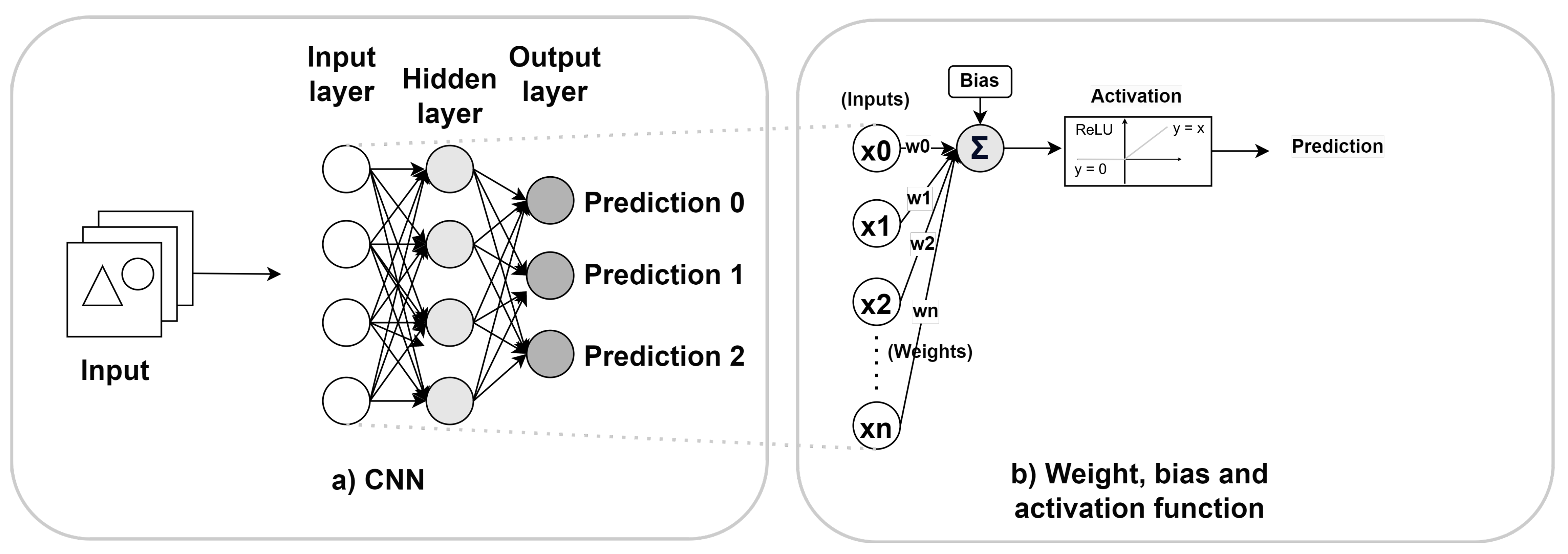
2.5. Convolutional Neural Networks
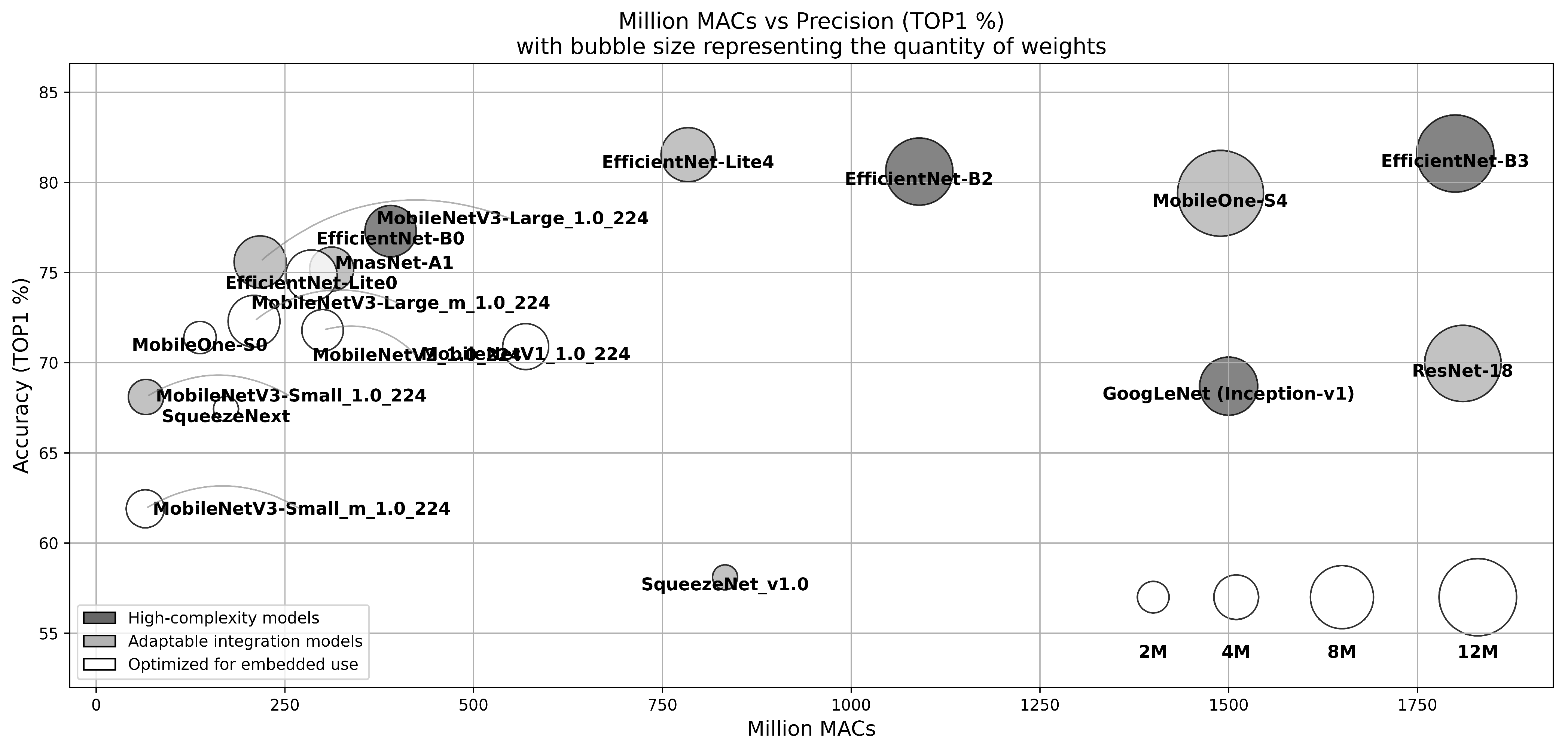
2.6. Evolution of Embedded Convolutional Neural Networks
- High-Complexity Models (dark gray): These models feature advanced topology and excellent accuracy but require significant layer modifications to adapt to embedded vision systems. These adaptations may include modifying or removing specific components such as Squeeze-and-Excite modules [76] or Swish activation [77] to make better use of complexity-reduction techniques. These models also require potential adaptation in terms of the number of parameters and calculations, which may not be suitable for certain embedded platforms.
- Adaptable Integration Models (light gray): This category includes designs that achieve high accuracy and maintain a manageable computing footprint. However, these models often require adaptations, such as modifications to certain layers, due to the large number of parameters and the computing power they require.
- Optimized for Embedded Use (White): These models are designed specifically for embedded systems, with an emphasis on ease of integration and minimal computational requirements. They use simple computation methods, such as ReLU activation, convolution factorization, and depth-separable convolutions [78], and incorporate techniques such as batch normalization [79] directly into the convolutional layers, as demonstrated by EfficientNet-Lite [59]. Although they can sometimes sacrifice accuracy, their low resource requirements make them ideal for resource-constrained environments.
2.7. AI Processing Unit
2.7.1. Flexibility
- High-flexibility approach: This approach imposes few or no restrictions on the choice of CNNs, allowing for a wide range of models and therefore facilitating a large number of applications.
- Moderate-flexibility approach: This approach focuses on a specific subset of convolutional neural networks, resulting in restrictions on the models and layers available, thus reducing the scope of potential applications.
- Low-flexibility approach: In this approach, the focus is on a particular CNN model, which severely limits adaptability in terms of model architecture and the range of applicable use cases.
2.7.2. Programmability
2.7.3. Software Stacks
2.7.4. AI Processing Unit Types
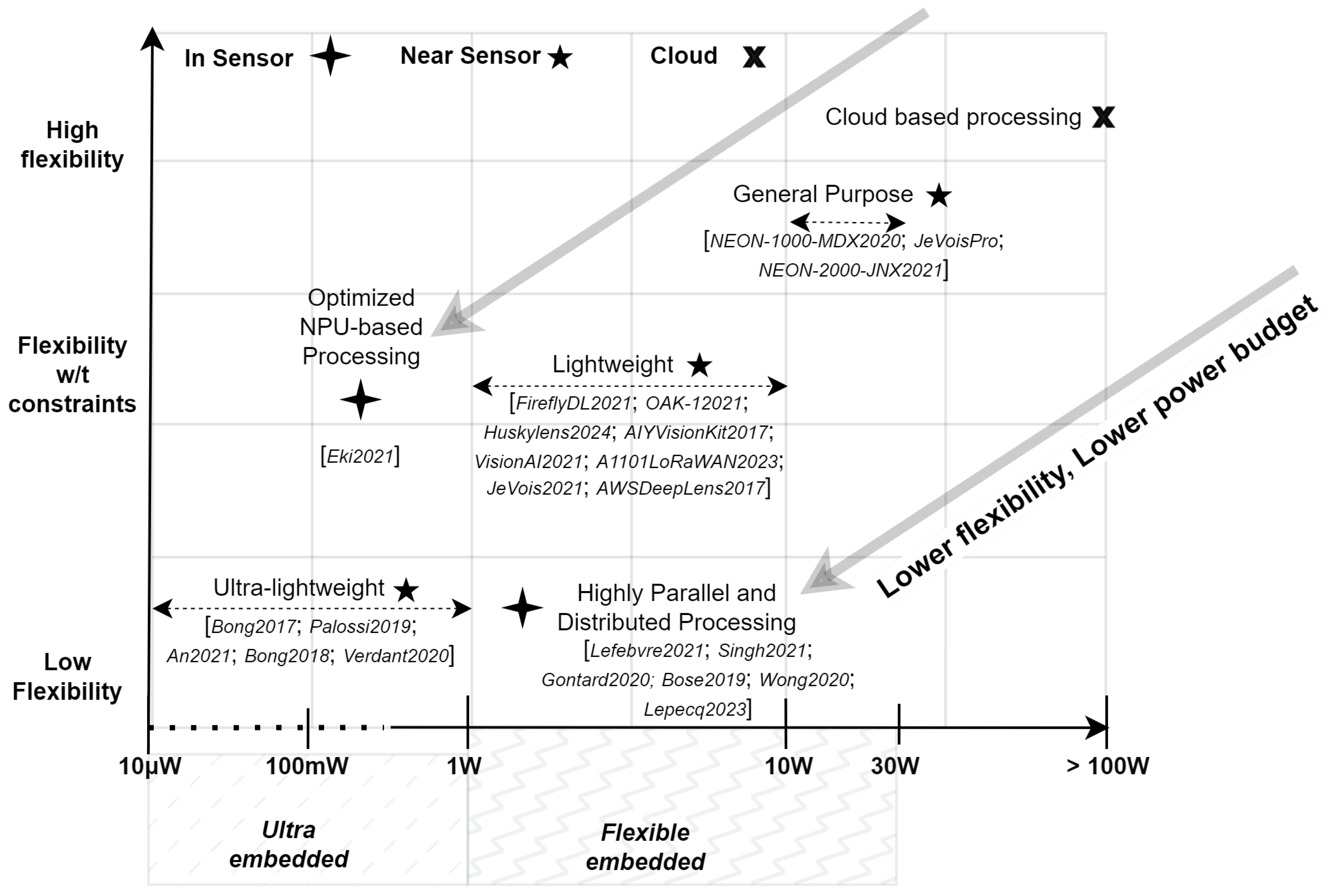
- General-purpose systems: Using architectures such as CPUs, GPUs, and FPGAs, these systems are characterized by their larger size and ability to deliver high performance across a wide range of AI processing tasks. Although they offer great flexibility and substantial computing power, this comes at the price of their increased power consumption and larger size. They are well suited to the use of full-featured software [95,96] for CNN implementation.
- Lightweight Systems: These systems employ specialized computing architectures like less powerful CPUs [98] or advanced NPUs [36] that focus on energy efficiency for particular tasks. Designed to achieve a balance between performance and power consumption, these architectures are suitable for environments where the highest levels of computational power are not necessary. They often use highly optimized dataflow and specialized software stacks such as TensorFlow Lite [99] and Spinnaker SDK Teledyne [100], tailored for specific, low-power AI applications.
- Ultra-lightweight systems: These systems employ specific computing and processing architectures that are generally designed for a single task, allowing a maximum compromise in favor of systems power consumption and at the expense of system flexibility [30].
2.8. Complexity-Reduction Techniques
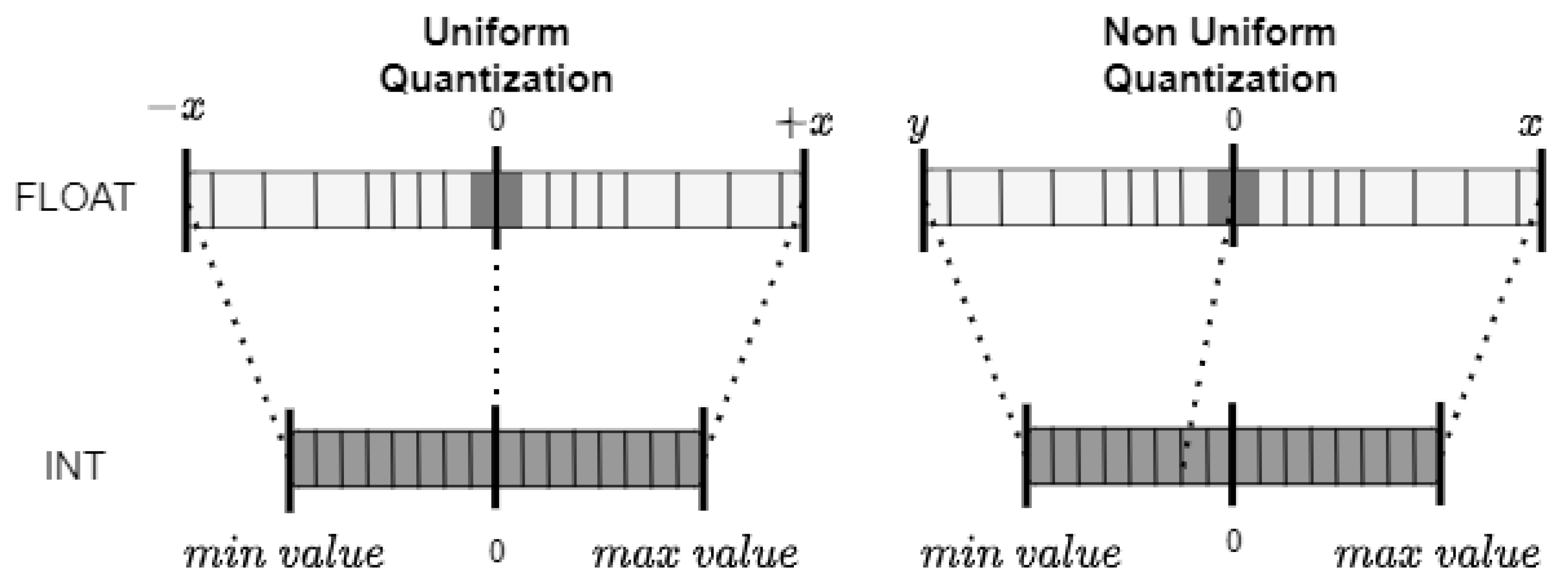
2.8.1. Quantization
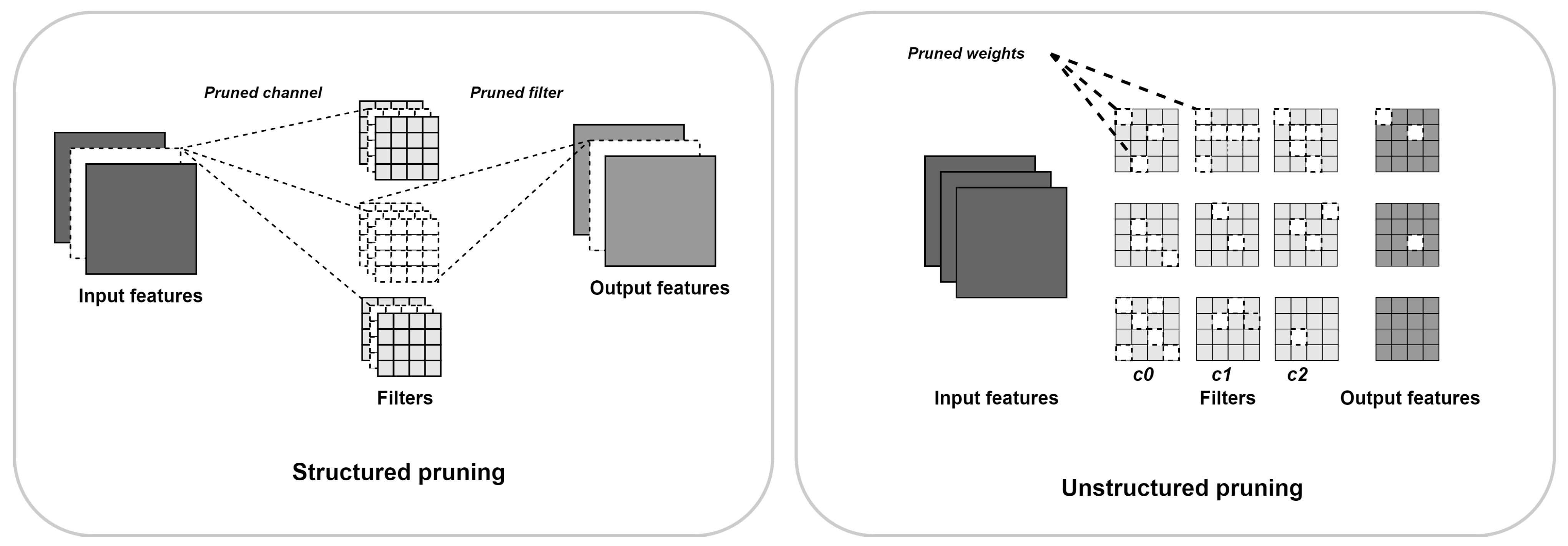
2.8.2. Pruning
2.8.3. AI Vision System Metrics
2.8.4. Frames per Second
2.8.5. System Size
2.8.6. Energy Consumption (Watts)
2.8.7. Energy Efficiency (TOPS/Watt)
2.8.8. Utilization Rate
2.9. Concluding Insights on Metrics and Characteristics of Embedded AI Vision Systems
3. Near-Sensor AI Vision Systems
- General-purpose AI vision systems are designed for high flexibility approaches, requiring significant computing power of general-purpose processing units to process high-complexity models.
- Lightweight AI vision systems are designed for a moderate-flexibility approach to simpler tasks, using less sophisticated adaptable integration models and reduced computing resources with lightweight processing units.
- Ultra-lightweight AI vision systems are designed for low-flexibility approaches and minimal power consumption and size with ultra-lightweight processing units, using basic CNN models optimized for embedded use and minimal processing capabilities.
3.1. General-Purpose AI Vision Systems
3.2. Lightweight AI Vision Systems
3.3. Ultra-Lightweight AI Vision Systems
3.4. Conclusion on Near-Sensor Processing AI Vision Systems
4. In-Sensor AI Vision Systems
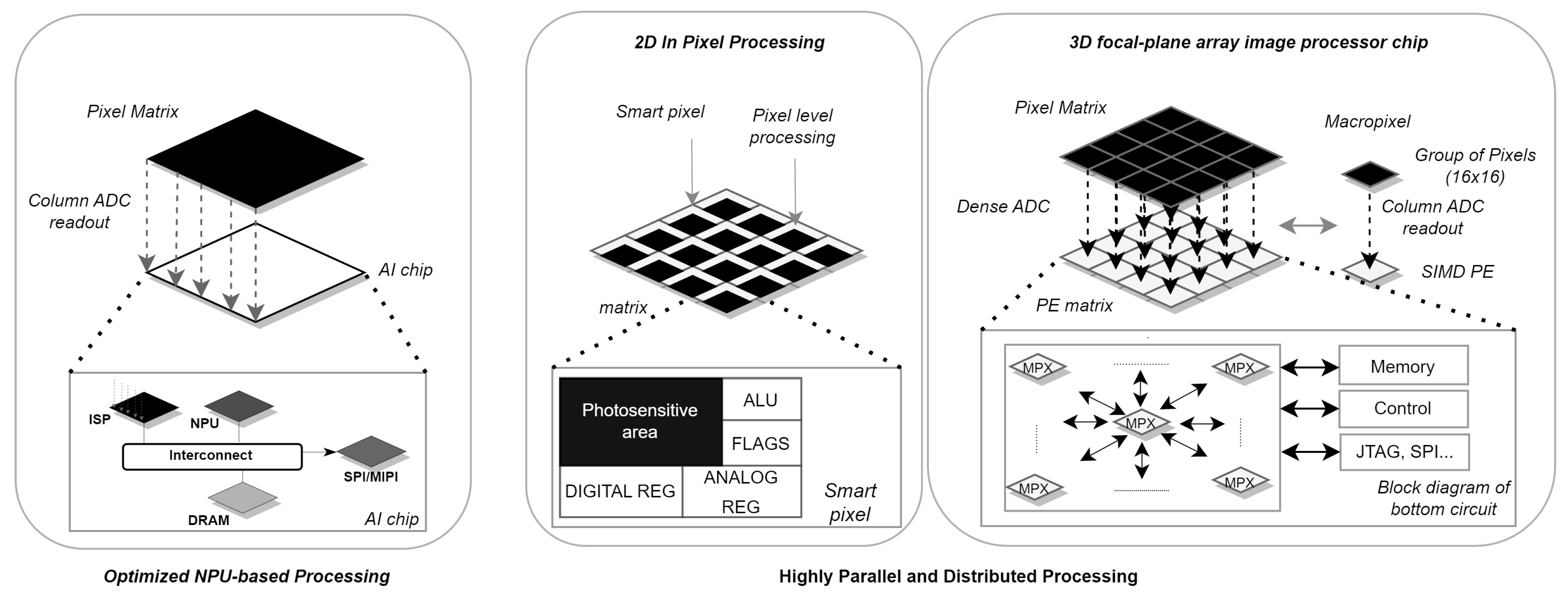
4.1. Introduction to 3D IC Vision Systems
4.2. Optimized NPU-Based Processing
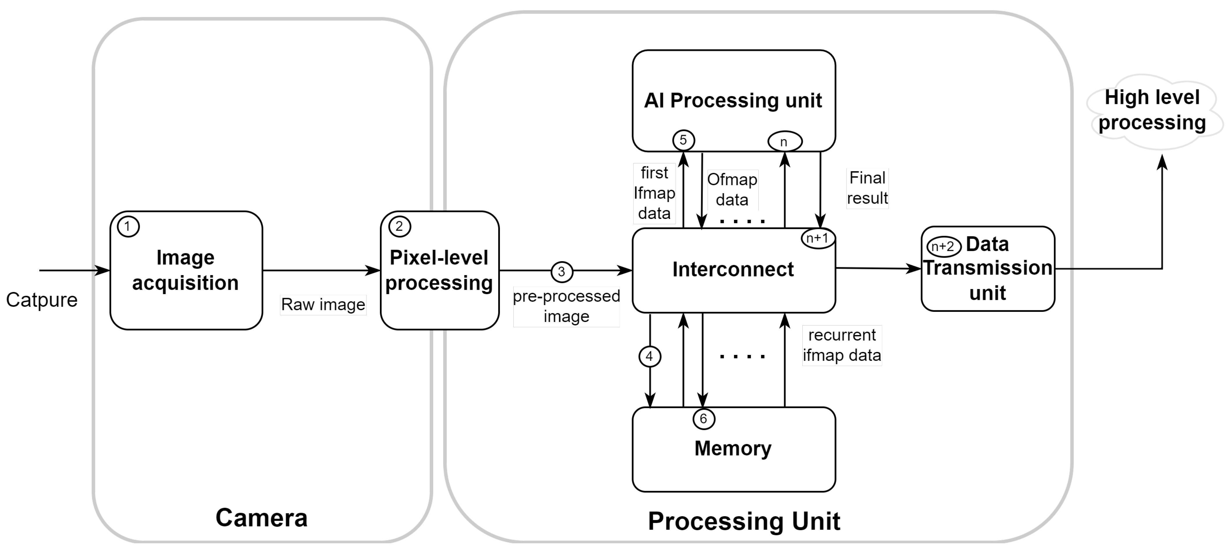
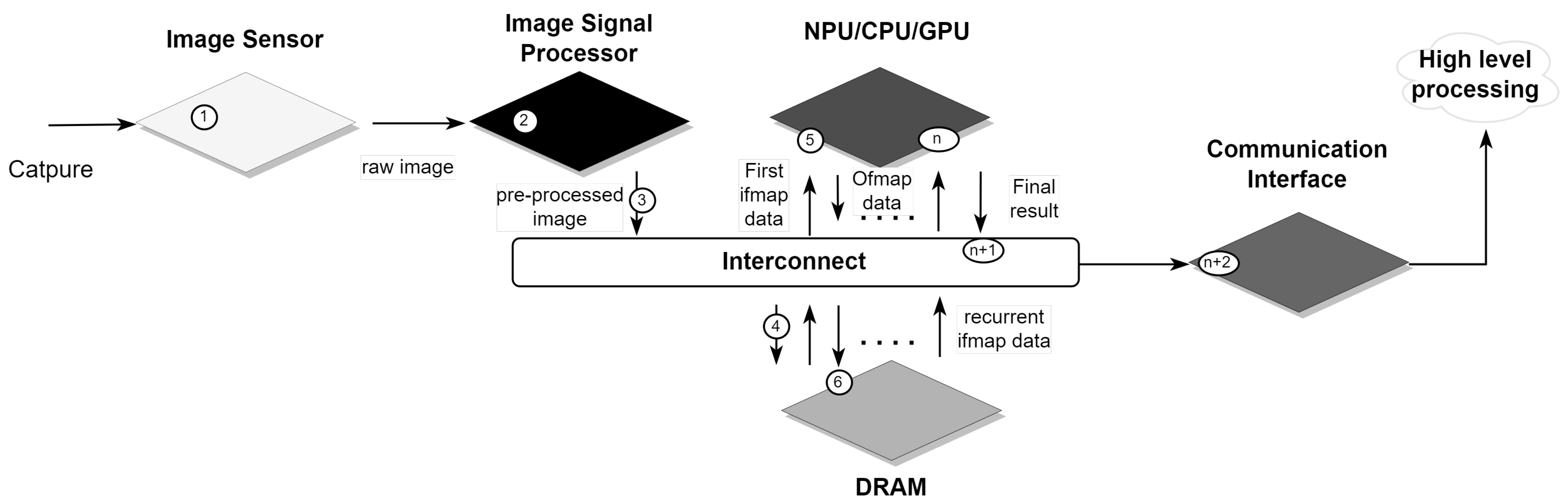
4.2.1. CNN Inference Process
4.2.2. Opportunities for Improvement
4.3. Two-dimensional In-Pixel Processing
4.3.1. CNN Inference Process
4.3.2. Opportunities for Improvement
4.4. Three-Dimensional Focal-Plane Array Image Processor Chip
4.4.1. CNN Inference Process
4.4.2. Opportunities for Improvement
4.5. Conclusion on In-Sensor Processing AI Vision Systems
5. Conclusions
5.1. Near-Sensor Systems
5.2. In-Sensor Systems
6. Perspectives
Author Contributions
Funding
Institutional Review Board Statement
Informed Consent Statement
Data Availability Statement
Conflicts of Interest
References
- Beckman, P.; Sankaran, R.; Catlett, C.; Ferrier, N.; Jacob, R.; Papka, M. Waggle: An open sensor platform for edge computing. In Proceedings of the 2016 IEEE Sensors, Orlando, FL, USA, 30 October–3 November 2016; pp. 1–3. [Google Scholar] [CrossRef]
- Theuwissen, A. There’s More to the Picture Than Meets the Eye and in the Future It Will Only Become More so. In Proceedings of the 2021 IEEE International Solid-State Circuits Conference (ISSCC), San Francisco, CA, USA, 13–22 February 2021; Volume 64, pp. 30–35. [Google Scholar] [CrossRef]
- Lowe, D.G. Distinctive Image Features from Scale-Invariant Keypoints. Int. J. Comput. Vis. 2004, 60, 91–110. [Google Scholar] [CrossRef]
- Bay, H.; Ess, A.; Tuytelaars, T.; Gool, L.V. Speeded-Up Robust Features (SURF). Comput. Vis. Image Underst. 2008, 110, 346–359. [Google Scholar] [CrossRef]
- Dalal, N.; Triggs, B. Histograms of oriented gradients for human detection. In Proceedings of the 2005 IEEE Computer Society Conference on Computer Vision and Pattern Recognition (CVPR’05), San Diego, CA, USA, 20–25 June 2005; Volume 1, pp. 886–893. [Google Scholar] [CrossRef]
- Deng, B.L.; Li, G.; Han, S.; Shi, L.; Xie, Y. Model Compression and Hardware Acceleration for Neural Networks: A Comprehensive Survey. Proc. IEEE 2020, 108, 485–532. [Google Scholar] [CrossRef]
- Sze, V.; Chen, Y.H.; Yang, T.J.; Emer, J.S. Efficient Processing of Deep Neural Networks: A Tutorial and Survey. Proc. IEEE 2017, 105, 2295–2329. [Google Scholar] [CrossRef]
- Capra, M.; Bussolino, B.; Marchisio, A.; Shafique, M.; Masera, G.; Martina, M. An Updated Survey of Efficient Hardware Architectures for Accelerating Deep Convolutional Neural Networks. Future Internet 2020, 12, 113. [Google Scholar] [CrossRef]
- Deng, J.; Dong, W.; Socher, R.; Li, L.-J.; Li, K.; Li, F.-F. Imagenet: A large-scale hierarchical image database. In Proceedings of the 2009 IEEE Conference on Computer Vision and Pattern Recognition, Miami, FL, USA, 20–25 June 2009; IEEE: Piscataway, NJ, USA, 2009; pp. 248–255. [Google Scholar] [CrossRef]
- Lin, T.Y.; Maire, M.; Belongie, S.; Bourdev, L.; Girshick, R.; Hays, J.; Perona, P.; Ramanan, D.; Zitnick, C.L.; Dollár, P. Microsoft COCO: Common Objects in Context. In Proceedings of the European Conference on Computer Vision (ECCV), Zurich, Switzerland, 6–12 September 2014; Springer: Cham, Switzerland, 2015; pp. 740–755. [Google Scholar] [CrossRef]
- Krizhevsky, A.; Sutskever, I.; Hinton, G.E. ImageNet Classification with Deep Convolutional Neural Networks. In Advances in Neural Information Processing Systems; Pereira, F., Burges, C.J.C., Bottou, L., Weinberger, K.Q., Eds.; Curran Associates, Inc.: Red Hook, NY, USA, 2012; Volume 25, pp. 1097–1105. [Google Scholar] [CrossRef]
- Minaee, S.; Boykov, Y.; Porikli, F.; Plaza, A.; Kehtarnavaz, N.; Terzopoulos, D. Image Segmentation Using Deep Learning: A Survey. IEEE Trans. Pattern Anal. Mach. Intell. 2021. [Google Scholar] [CrossRef]
- Zaidi, S.S.A.; Ansari, M.S.; Aslam, A.; Kanwal, N.; Asghar, M.; Lee, B. A Survey of Modern Deep Learning Based Object Detection Models. Digital Signal Processing 2022, 126, 103514. [Google Scholar] [CrossRef]
- He, K.; Zhang, X.; Ren, S.; Sun, J. Deep Residual Learning for Image Recognition. In Proceedings of the IEEE Conference on Computer Vision and Pattern Recognition (CVPR), Las Vegas, NV, USA, 27–30 June 2016; pp. 770–778. [Google Scholar] [CrossRef]
- Tolstikhin, I.O.; Houlsby, N.; Kolesnikov, A.; Beyer, L.; Zhai, X.; Unterthiner, T.; Yung, J.; Steiner, A.; Keysers, D.; Uszkoreit, J.; et al. MLP-Mixer: An all-MLP Architecture for Vision. In Proceedings of the Advances in Neural Information Processing Systems, NeurIPS, Online, 6–14 December 2021; pp. 24261–24272. Available online: https://proceedings.neurips.cc/paper/2021/hash/cba0a4ee5ccd02fda0fe3f9a3e7b89fe-Abstract.html (accessed on 15 July 2024).
- Touvron, H.; Bojanowski, P.; Caron, M.; Cord, M.; El-Nouby, A.; Grave, E.; Izacard, G.; Joulin, A.; Synnaeve, G.; Verbeek, J.; et al. ResMLP: Feedforward networks for image classification with data-efficient training. IEEE Trans. Pattern Anal. Mach. Intell. 2022, 45, 5314–5321. [Google Scholar] [CrossRef]
- Dosovitskiy, A.; Beyer, L.; Kolesnikov, A.; Weissenborn, D.; Zhai, X.; Unterthiner, T.; Dehghani, M.; Minderer, M.; Heigold, G.; Gelly, S.; et al. An Image is Worth 16x16 Words: Transformers for Image Recognition at Scale. In Proceedings of the International Conference on Learning Representations (ICLR), Vienna, Austria, 4 May 2021. [Google Scholar] [CrossRef]
- Touvron, H.; Cord, M.; Douze, M.; Massa, F.; Sablayrolles, A.; Jégou, H. Training data-efficient image transformers & distillation through attention. In Proceedings of the 38th International Conference on Machine Learning, Virtual, 18–24 July 2021. [Google Scholar]
- Liu, Z.; Lin, Y.; Cao, Y.; Hu, H.; Wei, Y.; Zhang, Z.; Lin, S.; Guo, B. Swin Transformer: Hierarchical Vision Transformer using Shifted Windows. In Proceedings of the IEEE/CVF International Conference on Computer Vision (ICCV), Montreal, QC, Canada, 10–17 October 2021; pp. 9992–10002. [Google Scholar] [CrossRef]
- Chen, S.; Xie, E.; Ge, C.; Chen, R.; Liang, D.; Luo, P. CycleMLP: A MLP-Like Architecture for Dense Visual Predictions. IEEE Trans. Pattern Anal. Mach. Intell. 2023, 45, 14284–14300. [Google Scholar] [CrossRef]
- Liu, H.; Dai, Z.; So, D.R.; Le, Q.V. Pay Attention to MLPs. In Advances in Neural Information Processing Systems; NeurIPS: Denver, CO, USA, 2021; pp. 9204–9215. [Google Scholar]
- Horowitz, M. 1.1 Computing’s Energy Problem (and What We Can Do about It). In Proceedings of the 2014 IEEE International Solid-State Circuits Conference Digest of Technical Papers (ISSCC), San Francisco, CA, USA, 9–13 February 2014; pp. 10–14. [Google Scholar] [CrossRef]
- Lepecq, M.; Dalgaty, T.; Fabre, W.; Chevobbe, S. End-to-End Implementation of a Convolutional Neural Network on a 3D-Integrated Image Sensor with Macropixel Array. Sensors 2023, 23, 1909. [Google Scholar] [CrossRef]
- Liu, P.; Yang, Z.; Kang, L.; Wang, J. A Heterogeneous Architecture for the Vision Processing Unit with a Hybrid Deep Neural Network Accelerator. Micromachines 2022, 13, 268. [Google Scholar] [CrossRef] [PubMed]
- Zheng, X.; Cheng, L.; Zhao, M.; Luo, Q.; Li, H.; Dou, R.; Yu, S.; Wu, N. ViP: A Hierarchical Parallel Vision Processor for Hybrid Vision Chip. IEEE Trans. Circuits Syst. II Express Briefs 2022, 69, 2957–2961. [Google Scholar] [CrossRef]
- Khronos Group. OpenCL: The Open Standard for Parallel Programming of Heterogeneous Systems. Available online: https://www.khronos.org/opencl/ (accessed on 3 April 2023).
- NVIDIA Corporation. CUDA Documentation. Available online: https://docs.nvidia.com/cuda/ (accessed on 3 April 2023).
- NVIDIA Corporation. TensorRT Documentation. Available online: https://developer.nvidia.com/tensorrt (accessed on 3 April 2023).
- ADLINK Technology. NEON-1000-MDX Starter Kit Series Datasheet. 2020. Available online: https://www.adlinktech.com/Products/Machine_Vision/SmartCamera/NEON-1000-MDX_Series (accessed on 3 April 2023).
- Garofalo, A.; Rusci, M.; Conti, F.; Rossi, D.; Benini, L. PULP-NN: Accelerating Quantized Neural Networks on Parallel Ultra-Low-Power RISC-V Processors. In Proceedings of the 26th IEEE International Conference on Electronics, Circuits and Systems (ICECS), Genoa, Italy, 27–29 November 2019; pp. 33–36. [Google Scholar] [CrossRef]
- Eki, R.; Yamada, S.; Ozawa, H.; Kai, H.; Okuike, K.; Gowtham, H.; Nakanishi, H.; Almog, E.; Livne, Y.; Yuval, G.; et al. 9.6 a 1/2.3inch 12.3Mpixel with on-Chip 4.97TOPS/W CNN Processor Back-Illuminated Stacked CMOS Image Sensor. In Proceedings of the 2021 IEEE International Solid-State Circuits Conference (ISSCC), San Francisco, CA, USA, 13–22 February 2021; Volume 64, pp. 154–156. [Google Scholar] [CrossRef]
- Bong, K.; Choi, S.; Kim, C.; Kang, S.; Kim, Y.; Yoo, H.J. 14.6 a 0.62mW Ultra-Low-Power Convolutional-Neural-Network facial recognition Processor and a CIS Integrated with Always-on Haar-like Face Detector. In Proceedings of the 2017 IEEE International Solid-State Circuits Conference (ISSCC), San Francisco, CA, USA, 5–9 February 2017; pp. 248–249. [Google Scholar] [CrossRef]
- Palossi, D.; Loquercio, A.; Conti, F.; Flamand, E.; Scaramuzza, D.; Benini, L. A 64-mW DNN-based Visual Navigation Engine for Autonomous Nano-Drones. IEEE Internet Things J. 2019, 6, 8357–8371. [Google Scholar] [CrossRef]
- JeVois. JeVois Pro: Smart Embedded Vision Toolkit. Available online: http://jevois.org/doc/ProUserConnect.html (accessed on 3 April 2023).
- Teledyne. FireflyDL Datasheet. 2021. Available online: https://www.flir.com/support-center/iis/machine-vision/knowledge-base/technical-documentation-firefly-s/ (accessed on 3 April 2023).
- Luxonis. OAK-1 DepthAI Hardware Product Page. 2021. Available online: https://shop.luxonis.com/products/oak-1?variant=42664380334303 (accessed on 20 August 2024).
- Bose, L.; Dudek, P.; Chen, J.; Carey, S.; Everitt, P.; Wang, H.; Davies, P.; Liu, J.; Wang, Y.; Uusitalo, A. A Camera That Cnns: Towards Embedded Neural Networks on Pixel Processor Arrays. In Proceedings of the 2019 IEEE/CVF International Conference on Computer Vision (ICCV), Seoul, Republic of Korea, 27 February 2019; pp. 1335–1344. [Google Scholar] [CrossRef]
- ADLINK Technology. NEON-2000-JNX Series Datasheet. 2021. Available online: https://www.adlinktech.com/Products/Machine_Vision/SmartCamera/NEON-2000-JNX_Series (accessed on 18 August 2024).
- DFRobot. Huskylens AI Machine Vision Sensor. 2024. Available online: https://store-usa.arduino.cc/products/gravity-huskylens-ai-machine-vision-sensor (accessed on 3 August 2024).
- AIY, G. AIY Vision Kit v1.1. 2024. Available online: https://pi3g.com/products/machine-learning/google-coral/aiy-vision-kit/ (accessed on 3 August 2024).
- ImagoTechnologies. VisionAI v1.2 Datasheet. 2021. Available online: https://imago-technologies.com/wp-content/uploads/2021/01/Specification-VisionAI-V1.2.pdf (accessed on 3 August 2023).
- Seeed Studio. SenseCAP A1101 LoRaWAN Vision AI Sensor User Guide. 2024. Available online: https://files.seeedstudio.com/wiki/SenseCAP-A1101/SenseCAP_A1101_LoRaWAN_Vision_AI_Sensor_User_Guide_V1.0.2.pdf (accessed on 18 August 2024).
- JeVois. JeVois Smart Machine. Available online: https://www.jevoisinc.com/pages/hardware (accessed on 3 April 2023).
- Amazon Web Services. AWS DeepLens AI Vision. 2024. Available online: https://bloggeek.me/aws-deeplens-ai-vision/ (accessed on 4 August 2024).
- An, H.; Schiferl, S.; Venkatesan, S.; Wesley, T.; Zhang, Q.; Wang, J.; Choo, K.D.; Liu, S.; Li, Z.; Gong, L. An Ultra-Low-Power Image Signal Processor for Hierarchical Image Recognition with Deep Neural Networks. IEEE J. Solid-State Circuits 2021, 56, 1071–1081. [Google Scholar] [CrossRef]
- Bong, K.; Choi, S.; Kim, C.; Han, D.; Yoo, H.-J. A Low-Power Convolutional Neural Network Face Recognition Processor and a CIS Integrated with Always-on Face Detector. IEEE J. Solid-State Circuits 2018, 53, 115–123. [Google Scholar] [CrossRef]
- Verdant, A.; Guicquero, W.; Royer, N.; Moritz, G.; Seifert, T.; Hsu, C.-H.; He, Z. A 3.0μW5fps QQVGA Self-Controlled Wake-up Imager with on-Chip Motion Detection, Auto-Exposure and Object Recognition. In Proceedings of the 2020 IEEE Symposium on VLSI Circuits, Honolulu, HI, USA, 16–19 June 2020; pp. 1–2. [Google Scholar] [CrossRef]
- Lefebvre, M.; Moreau, L.; Dekimpe, R.; Bol, D. A 0.2-to-3.6TOPS/W Programmable Convolutional Imager SoC with in-Sensor Current-Domain Ternary-Weighted MAC Operations for Feature Extraction and Region-of-Interest Detection. In Proceedings of the 2021 IEEE International Solid-State Circuits Conference (ISSCC), San Francisco, CA, USA, 13–22 February 2021; Volume 64, pp. 118–120. [Google Scholar] [CrossRef]
- Singh, R.; Bailey, S.; Chang, P.; Olyaei, A.; Hekmat, M.; Winoto, R. 34.2 A 21pJ/frame/pixel Imager and 34pJ/frame/pixel Image Processor for a Low-Vision Augmented-Reality Smart Contact Lens. In Proceedings of the 2021 IEEE International Solid-State Circuits Conference (ISSCC), San Francisco, CA, USA, 13–22 February 2021; Volume 64, pp. 482–484. [Google Scholar] [CrossRef]
- Wong, M.Z.; Guillard, B.; Murai, R.; Saeedi, S.; Kelly, P.H.J. AnalogNet: Convolutional Neural Network Inference on Analog Focal Plane Sensor Processors. arXiv 2020, arXiv:2006.01765. Available online: http://arxiv.org/abs/2006.01765 (accessed on 18 August 2024).
- Gontard, L.C.; Carmona-Galan, R.; Rodriguez-Vazquez, A. Cellular-Neural-Network Focal-Plane Processor as Pre-Processor for ConvNet Inference. In Proceedings of the 2020 IEEE International Symposium on Circuits and Systems (ISCAS), Seville, Spain, 12–14 October 2020; pp. 1–5. [Google Scholar] [CrossRef]
- Oike, Y. Evolving Image Sensor Architecture through Stacking Devices. IEEE Trans. Electron Devices 2021, 68, 5535–5543. [Google Scholar] [CrossRef]
- Carey, S.J.; Lopich, A.; Barr, D.R.W.; Wang, B.; Dudek, P. A 100,000 fps Vision Sensor with Embedded 535GOPS/W 256×256 SIMD Processor Array. In Proceedings of the 2013 Symposium on VLSI Circuits, Kyoto, Japan, 12–14 June 2013; pp. C182–C183. [Google Scholar]
- Rodríguez-Vázquez, Á.; Fernández-Berni, J.; Leñero-Bardallo, J.A.; Vornicu, I.; Carmona-Galán, R. CMOS Vision Sensors: Embedding Computer Vision at Imaging Front-Ends. IEEE Circuits Syst. Mag. 2018, 18, 90–107. [Google Scholar] [CrossRef]
- Millet, L.; Chevobbe, S.; Andriamisaina, C.; Beigné, E.; Benaissa, L.; Deschaseaux, E.; Benchehida, K.; Lepecq, M.; Darouich, M.; Guellec, F.; et al. A 5500FPS 85GOPS/W 3D Stacked BSI Vision Chip Based on Parallel in-Focal-Plane Acquisition and Processing. In Proceedings of the 2018 IEEE Symposium on VLSI Circuits, Honolulu, HI, USA, 18–22 June 2018; pp. 245–246. [Google Scholar] [CrossRef]
- Li, W.; Manley, M.; Read, J.; Kaul, A.; Bakir, M.S.; Yu, S. H3DAtten: Heterogeneous 3-D Integrated Hybrid Analog and Digital Compute-in-Memory Accelerator for Vision Transformer Self-Attention. IEEE Trans. Very Large Scale Integr. (VLSI) Syst. 2023, 31, 1592–1602. [Google Scholar] [CrossRef]
- Mukhopadhyay, S.; Long, Y.; Mudassar, B.; Nair, C.S.; DeProspo, B.H.; Torun, H.M.; Kathaperumal, M.; Smet, V.; Kim, D.; Yalamanchili, S.; et al. Heterogeneous Integration for Artificial Intelligence: Challenges and Opportunities. IBM J. Res. Dev. 2019, 63, 4:1–4:23. [Google Scholar] [CrossRef]
- Howard, A.G.; Zhu, M.; Chen, B.; Kalenichenko, D.; Wang, W.; Weyand, T.; Andreetto, M.; Adam, H. MobileNets: Efficient Convolutional Neural Networks for Mobile Vision Applications. arXiv 2017, arXiv:1704.04861. Available online: http://arxiv.org/abs/1704.04861 (accessed on 18 August 2024).
- Tan, M.; Le, Q.V. EfficientNet: Rethinking Model Scaling for Convolutional Neural Networks. In Proceedings of the 36th International Conference on Machine Learning, PMLR 97:6105–6114, Long Beach, CA, USA, 9–15 June 2019. [Google Scholar]
- Xu, C.; Mo, Y.; Ren, G.; Ma, W.; Wang, X.; Shi, W.; Hou, J.; Shao, K.; Wang, H.; Xiao, P.; et al. 5.1 A Stacked Global-Shutter CMOS Imager with SC-Type Hybrid-GS Pixel and Self-Knee Point Calibration Single Frame HDR and On-Chip Binarization Algorithm for Smart Vision Applications. In Proceedings of the 2019 IEEE International Solid-State Circuits Conference (ISSCC), San Francisco, CA, USA, 17–21 February 2019; pp. 94–96. [Google Scholar] [CrossRef]
- Viola, P.; Jones, M. Rapid object detection using a boosted cascade of simple features. In Proceedings of the 2001 IEEE Computer Society Conference on Computer Vision and Pattern Recognition (CVPR), Kauai, HI, USA, 8–14 December 2001; Volume 1, pp. I-511–I-518. [Google Scholar] [CrossRef]
- Chevobbe, S.; Lepecq, M.; Benchehida, K.; Darouich, M.; Dombek, T.; Guellec, F.; Millet, L. A Versatile 3D Stacked Vision Chip with Massively Parallel Processing Enabling Low Latency Image Analysis. In Proceedings of the 2019 International Image Sensor Workshop, Snowbird, UT, USA, 23–27 June 2019; Available online: https://api.semanticscholar.org/CorpusID:210114478 (accessed on 18 August 2024).
- Tsugawa, H.; Takahashi, H.; Nakamura, R.; Umebayashi, T.; Ogita, T.; Okano, H.; Nomoto, T. Pixel/DRAM/Logic 3-Layer Stacked CMOS Image Sensor Technology. In Proceedings of the 2017 IEEE International Electron Devices Meeting (IEDM), San Francisco, CA, USA, 2–6 December 2017; pp. 3.2.1–3.2.4. [Google Scholar] [CrossRef]
- Haruta, T.; Nakajima, T.; Hashizume, J.; Umebayashi, T.; Gotoh, Y.; Maeda, S.; Kaneko, M.; Morimoto, S.; Murakami, K.; Iwahashi, S. 4.6 a 1/2.3inch 20mpixel 3-Layer Stacked CMOS Image Sensor with DRAM. In Proceedings of the 2017 IEEE International Solid-State Circuits Conference (ISSCC), San Francisco, CA, USA, 5–9 February 2017; pp. 76–77. [Google Scholar] [CrossRef]
- PCI-SIG. PCI Express Base Specification Revision 5.0, Version 1.0. PCI-SIG. 2024. Available online: https://pcisig.com/specifications/pciexpress/ (accessed on 20 August 2024).
- NVIDIA. Jetson AGX Xavier Developer Kit User Guide. NVIDIA Corporation, Online Resource. Available online: https://developer.nvidia.com/embedded/downloads (accessed on 20 August 2024).
- MIPI Alliance. MIPI CSI-2 Specification Version 4.0. MIPI Alliance. 2024. Available online: https://www.mipi.org/specifications/csi-2 (accessed on 20 August 2024).
- Google. Coral Edge TPU Datasheet. Google, Online Resource. Available online: https://coral.ai/products/edgetpu/ (accessed on 3 April 2023).
- Bonnin, P.; Blazevic, P.; Pissaloux, E.; Al Nachar, R. Methodology of Evaluation of Low Cost Electronic Devices: Raspberry PI and Nvidia Jetson Nano for Perception System Implementation in Robotic Applications. In Proceedings of the 2022 IEEE Information Technologies & Smart Industrial Systems (ITSIS), Paris, France, 15–17 July 2022; pp. 1–6. [Google Scholar] [CrossRef]
- Arm Limited. AMBA AXI and ACE Protocol Specification Version 4.0. Arm Limited. 2024. Available online: https://developer.arm.com/documentation/ihi0022/g (accessed on 20 August 2024).
- NXP Semiconductors. I2C Bus Specification and User Manual, Revision 7. NXP Semiconductors. 2024. Available online: https://www.nxp.com/docs/en/user-guide/UM10204.pdf (accessed on 20 August 2024).
- VTI Technologies. TN15 SPI Interface Specification. VTI Technologies. 2005. Available online: https://www.mouser.com/pdfdocs/tn15_spi_interface_specification.PDF (accessed on 20 August 2024).
- Lecun, Y.; Bottou, L.; Bengio, Y.; Haffner, P. Gradient-Based Learning Applied to Document Recognition. Proc. IEEE 1998, 86, 2278–2324. [Google Scholar] [CrossRef]
- Goodfellow, I.; Bengio, Y.; Courville, A. Deep Learning; MIT Press: Cambridge, MA, USA, 2016. [Google Scholar]
- Bianco, S.; Cadene, R.; Celona, L.; Napoletano, P. Benchmark Analysis of Representative Deep Neural Network Architectures. IEEE Access 2018, 6, 64270–64277. [Google Scholar] [CrossRef]
- Hu, J.; Shen, L.; Sun, G. Squeeze-and-Excitation Networks. In Proceedings of the IEEE Conference on Computer Vision and Pattern Recognition (CVPR), Salt Lake City, UT, USA, 18–22 June 2018; pp. 7132–7141. [Google Scholar] [CrossRef]
- Ramachandran, P.; Zoph, B.; Le, Q.V. Searching for Activation Functions. In Proceedings of the International Conference on Learning Representations (ICLR), Toulon, France, 24–26 April 2017. [Google Scholar]
- Chollet, F. Xception: Deep Learning with Depthwise Separable Convolutions. In Proceedings of the IEEE Conference on Computer Vision and Pattern Recognition (CVPR), Honolulu, HI, USA, 21–26 July 2017; pp. 1251–1258. [Google Scholar] [CrossRef]
- Ioffe, S.; Szegedy, C. Batch Normalization: Accelerating Deep Network Training by Reducing Internal Covariate Shift. In Proceedings of the 32nd International Conference on Machine Learning (ICML), Lille, France, 7–9 July 2015; pp. 448–456. [Google Scholar]
- Szegedy, C.; Liu, W.; Jia, Y.; Sermanet, P.; Reed, S.; Anguelov, D.; Erhan, D.; Vanhoucke, V.; Rabinovich, A. Going Deeper with Convolutions. In Proceedings of the IEEE Conference on Computer Vision and Pattern Recognition (CVPR), Boston, MA, USA, 7–12 June 2015; pp. 1–9. [Google Scholar] [CrossRef]
- Iandola, F.N.; Han, S.; Moskewicz, M.W.; Ashraf, K.; Dally, W.J.; Keutzer, K. SqueezeNet: AlexNet-level Accuracy with 50x Fewer Parameters and <0.5 MB Model Size. 2017. Available online: https://openreview.net/forum?id=S1xh5sYgx (accessed on 20 August 2024).
- Howard, A.; Sandler, M.; Chen, B.; Wang, W.; Chen, L.C.; Tan, M.; Chu, G.; Vasudevan, V.; Zhu, Y.; Pang, R. Searching for MobileNetV3. In Proceedings of the 2019 IEEE/CVF International Conference on Computer Vision (ICCV), Seoul, Republic of Korea, 27 October–2 November 2019; pp. 1314–1324. [Google Scholar] [CrossRef]
- Gholami, A.; Kwon, K.; Wu, B.; Tai, Z.; Yue, X.; Jin, P.; Zhao, S.; Keutzer, K. SqueezeNext: Hardware-Aware Neural Network Design. In Proceedings of the 2018 IEEE/CVF Conference on Computer Vision and Pattern Recognition Workshops (CVPRW), Salt Lake City, UT, USA, 18–22 June 2018; pp. 1719–171909. [Google Scholar] [CrossRef]
- Tan, M.; Chen, B.; Pang, R.; Vasudevan, V.; Sandler, M.; Howard, A.; Le, Q.V. MnasNet: Platform-Aware Neural Architecture Search for Mobile. In Proceedings of the 2019 IEEE/CVF Conference on Computer Vision and Pattern Recognition (CVPR), Long Beach, CA, USA, 16–20 June 2019; pp. 2815–2823. [Google Scholar] [CrossRef]
- Google AI Blog. Introducing the Next Generation of On-Device Vision Models: MobileNetV3 and MobileNetEdgeTPU. 2019. Available online: https://ai.googleblog.com/2019/11/introducing-next-generation-on-device.html (accessed on 3 April 2023).
- Sandler, M.; Howard, A.; Zhu, M.; Zhmoginov, A.; Chen, L.C. MobileNetV2: Inverted Residuals and Linear Bottlenecks. In Proceedings of the 2018 IEEE/CVF Conference on Computer Vision and Pattern Recognition (CVPR), Salt Lake City, UT, USA, 18–22 June 2018; pp. 4510–4520. [Google Scholar] [CrossRef]
- Simonyan, K.; Zisserman, A. Very Deep Convolutional Networks for Large-Scale Image Recognition. arXiv 2015, arXiv:1409.1556. Available online: http://arxiv.org/abs/1409.1556 (accessed on 18 August 2024).
- Mitchell, J.C. MobileNetV2 Keras Implementation. 2018. Available online: https://github.com/JonathanCMitchell/mobilenet_v2_keras/blob/master/mobilenetv2.py (accessed on 27 July 2024).
- White, C.; Safari, M.; Sukthanker, R.; Ru, B.; Lindauer, M.; Hutter, F. Neural Architecture Search: Insights from 1000 Papers. arXiv 2023, arXiv:2301.08727. Available online: https://arxiv.org/abs/2301.08727 (accessed on 18 August 2024).
- Keras Team. Keras Applications-MobileNet. 2023. Available online: https://keras.io/api/applications/mobilenet/ (accessed on 27 July 2024).
- TensorFlow Blog. Higher Accuracy on Vision Models with EfficientNet-Lite. 2020. Available online: https://blog.tensorflow.org/2020/03/higher-accuracy-on-vision-models-with-efficientnet-lite.html (accessed on 3 April 2023).
- Fukushima, K. Cognitron: A self-organizing multilayered neural network. Biol. Cybern. 1975, 20, 121–136. [Google Scholar] [CrossRef]
- Vasu, P.K.A.; Gabriel, J.; Zhu, J.; Tuzel, O.; Ranjan, A. MobileOne: An Improved One millisecond Mobile Backbone. In Proceedings of the 2023 IEEE/CVF Conference on Computer Vision and Pattern Recognition (CVPR), Vancouver, BC, Canada, 18–22 June 2023; pp. 7907–7917. [Google Scholar] [CrossRef]
- Amid, A.; Kwon, K.; Gholami, A.; Wu, B.; Keutzer, K.; Mahoney, M.W. Co-design of deep neural nets and neural net accelerators for embedded vision applications. IBM J. Res. Dev. 2019, 63, 6:1–6:14. [Google Scholar] [CrossRef]
- Abadi, M.; Barham, P.; Chen, J.; Chen, Z.; Davis, A.; Dean, J.; Devin, M.; Ghemawat, S.; Irving, G.; Isard, M.; et al. TensorFlow: A system for large-scale machine learning. In Proceedings of the 12th USENIX Symposium on Operating Systems Design and Implementation (OSDI), Savannah, GA, USA, 2–4 November 2016; pp. 265–283. [Google Scholar]
- Paszke, A.; Gross, S.; Massa, F.; Lerer, A.; Bradbury, J.; Chanan, G.; Killeen, T.; Lin, Z.; Gimelshein, N.; Antiga, L.; et al. PyTorch: An Imperative Style, High-Performance Deep Learning Library. In Proceedings of the 32nd Advances in Neural Information Processing Systems (NeurIPS), Vancouver, BC, Canada, 8–14 December 2019; Available online: https://proceedings.neurips.cc/paper_files/paper/2019/file/bdbca288fee7f92f2bfa9f7012727740-Paper.pdf (accessed on 20 August 2024).
- CEA-LIST. N2D2. Available online: https://github.com/CEA-LIST/N2D2 (accessed on 3 April 2024).
- Khadas. Khadas VIM3 Online Datasheet. 2021. Available online: https://docs.khadas.com/vim3/ (accessed on 3 April 2023).
- Google Research. TensorFlow Lite. Available online: https://www.tensorflow.org/lite (accessed on 3 April 2023).
- Teledyne. Spinnaker SDK Teledyne FLIR. 2021. Available online: https://www.flir.fr/products/spinnaker-sdk?vertical=machine+vision&segment=iis (accessed on 3 April 2023).
- Cheng, J.; Wu, J.; Leng, C.; Wang, Y.; Hu, Q.; Tao, D. Quantized CNN: A Unified Approach to Accelerate and Compress Convolutional Networks. IEEE Trans. Neural Netw. Learning Syst. 2018, 29, 4730–4743. [Google Scholar] [CrossRef]
- Krishnamoorthi, R. Quantizing Deep Convolutional Networks for Efficient Inference: A Whitepaper. arXiv 2018, arXiv:1806.08342. Available online: http://arxiv.org/abs/1806.08342 (accessed on 18 August 2024).
- Nagel, M.; Fournarakis, M.; Amjad, R.A.; Bondarenko, Y.; Blankevoort, T. A White Paper on Neural Network Quantization. arXiv 2021, arXiv:2106.08295. Available online: https://arxiv.org/abs/2106.08295 (accessed on 18 August 2024).
- Liang, T.; Glossner, J.; Wang, L.; Shi, S.; Zhang, X. Pruning and Quantization for Deep Neural Network Acceleration: A Survey. Neurocomputing 2021, 461, 370–403. [Google Scholar] [CrossRef]
- Han, S.; Pool, J.; Tran, J.; Dally, W.J. Learning Both Weights and Connections for Efficient Neural Networks. In Proceedings of the 28th International Conference on Neural Information Processing Systems (NIPS’15), Montreal, QC, Canada, 7–12 December 2015; pp. 1135–1143. Available online: https://proceedings.neurips.cc/paper_files/paper/2015/file/ae0eb3eed39d2bcef4622b2499a05fe6-Paper.pdf (accessed on 20 August 2024).
- Lin, M.; Ji, R.; Wang, Y.; Zhang, Y.; Tian, Y.; Shao, L. HRank: Filter Pruning Using High-Rank Feature Map. In Proceedings of the IEEE/CVF Conference on Computer Vision and Pattern Recognition (CVPR), Seattle, WA, USA, 13–19 June 2020; pp. 1529–1538. [Google Scholar] [CrossRef]
- Yvinec, E.; Dapogny, A.; Cord, M.; Bailly, K. RED: Looking for Redundancies for Data-Free Structured Compression of Deep Neural Networks. In Proceedings of the 35th International Conference on Neural Information Processing Systems (NIPS’21), Red Hook, NY, USA, 9–15 December 2024; Curran Associates Inc.: Red Hook, NY, USA, 2024. Available online: https://dl.acm.org/doi/10.5555/3540261.3541857 (accessed on 18 August 2024).
- Courbariaux, M.; Bengio, Y.; David, J.P. BinaryConnect: Training Deep Neural Networks with Binary Weights during Propagations. In Proceedings of the 28th International Conference on Neural Information Processing Systems (NIPS’15), Montreal, Canada, 7–12 December 2015; pp. 3123–3131. Available online: https://dl.acm.org/doi/10.5555/2969442.2969588 (accessed on 18 August 2024).
- Rastegari, M.; Ordonez, V.; Redmon, J.; Farhadi, A. Xnor-net: Imagenet classification using binary convolutional neural networks. In Proceedings of the European Conference on Computer Vision, Amsterdam, The Netherlands, 11–14 October 2016; Leibe, B., Matas, J., Sebe, N., Welling, M., Eds.; Springer International Publishing: Cham, Switzerland, 2016; Volume 9908, pp. 525–542. [Google Scholar] [CrossRef]
- Gholami, A.; Kim, S.; Dong, Z.; Yao, Z.; Mahoney, M.W.; Keutzer, K. A Survey of Quantization Methods for Efficient Neural Network Inference. CoRR 2021. Available online: https://arxiv.org/abs/2103.13630 (accessed on 18 August 2024).
- Grootendorst, M. A Visual Guide to Quantization. 2023. Available online: https://newsletter.maartengrootendorst.com/p/a-visual-guide-to-quantization (accessed on 4 August 2024).
- Nagel, M.; Amjad, R.A.; Van Baalen, M.; Louizos, C.; Blankevoort, T. Up or down? Adaptive rounding for post-training quantization. In Proceedings of the 37th International Conference on Machine Learning, Virtual, 13–18 July 2020; PMLR: Virtual; pp. 7197–7206. [Google Scholar]
- Li, Y.; Gong, R.; Tan, X.; Yang, Y.; Hu, P.; Zhang, Q.; Yu, F.; Wang, W.; Gu, S. BRECQ: Pushing the Limit of Post-Training Quantization by Block Reconstruction. In Proceedings of the International Conference on Learning Representations (ICLR), Virtual, 3–7 May 2021; Available online: https://iclr.cc/virtual/2021/poster/2596 (accessed on 18 August 2024).
- Xu, K.; Li, Z.; Wang, S.; Zhang, X. PTMQ: Post-training Multi-Bit Quantization of Neural Networks. In Proceedings of the AAAI Conference on Artificial Intelligence, Virtual, 18–22 November 2024; pp. 16193–16201. [Google Scholar] [CrossRef]
- Nahshan, Y.; Chmiel, B.; Baskin, C.; Zheltonozhskii, E.; Banner, R.; Bronstein, A.M.; Mendelson, A. Loss Aware Post-training Quantization. Mach. Learn. 2021, 110, 3245–3262. [Google Scholar] [CrossRef]
- Choi, J.; Wang, Z.; Venkataramani, S.; Chuang, P.I.J.; Srinivasan, V.; Gopalakrishnan, K. PACT: Parameterized Clipping Activation for Quantized Neural Networks. arXiv 2018, arXiv:1805.06085. Available online: https://arxiv.org/abs/1805.06085 (accessed on 18 August 2024).
- Chen, Y.H.; Krishna, T.; Emer, J.S.; Sze, V. Eyeriss: An Energy-Efficient Reconfigurable Accelerator for Deep Convolutional Neural Networks. IEEE J. Solid-State Circuits 2017, 52, 127–138. [Google Scholar] [CrossRef]
- NVIDIA. Jetson TX2 Module Online Datasheet. 2022. Available online: https://developer.nvidia.com/embedded/jetson-tx2 (accessed on 3 April 2023).
- Khadas. Khadas VIM4 Online Datasheet. Available online: https://www.khadas.com/vim4 (accessed on 3 April 2023).
- Reddi, V.J.; Cheng, C.; Kanter, D.; Mattson, P.; Schmuelling, G.; Wu, C.-J.; Anderson, B.; Breughe, M.; Charlebois, M.; Chou, W.; et al. MLPerf Inference Benchmark. CoRR 2019. Available online: https://arxiv.org/abs/1911.02549 (accessed on 18 August 2024).
- Allwinner Technology. A33 Datasheet. 2014. Available online: https://github.com/allwinner-zh/documents/blob/master/A33/A33%20Datasheet%20release%201.1.pdf (accessed on 3 April 2023).
- Intel. Intel Movidius Myriad X Vision Processing Unit (VPU). 2021. Available online: https://www.intel.com/content/www/us/en/products/details/processors/movidius-vpu/movidius-myriad-x.html (accessed on 3 April 2023).
- Liu, P.; Song, Y. A Hybrid Vision Processing Unit with a Pipelined Workflow for Convolutional Neural Network Accelerating and Image Signal Processing. Electronics 2021, 10, 2989. [Google Scholar] [CrossRef]
- Szegedy, C.; Vanhoucke, V.; Ioffe, S.; Shlens, J.; Wojna, Z. Rethinking the Inception Architecture for Computer Vision. In Proceedings of the IEEE Conference on Computer Vision and Pattern Recognition (CVPR), Las Vegas, NV, USA, 27–30 June 2016; pp. 2818–2826. [Google Scholar] [CrossRef]
- Teledyne. FireflyDL Online Datasheet: Neural Networks Supported by the Firefly DL. 2021. Available online: https://www.flir.com/support-center/iis/machine-vision/application-note/neural-networks-supported-by-the-firefly-dl/ (accessed on 3 April 2023).
- Nair, D.; Pakdaman, A.; Plöger, P.G. Performance Evaluation of Low-Cost Machine Vision Cameras for Image-Based Grasp Verification. arXiv 2020, arXiv:2003.10167. Available online: http://arxiv.org/abs/2003.10167 (accessed on 18 August 2024).
- GreenWaves Technologies. GAP8 CNN Benchmarks. Available online: https://greenwaves-technologies.com/gap8-cnn-benchmarks/ (accessed on 3 April 2023).
- Himax Technologies, Inc. Image Sensors by Himax Technologies, Inc. Available online: https://www.himax.com.tw/en/products/cmos-image-sensor/image-sensors/ (accessed on 3 April 2023).
- Loquercio, A.; Maqueda, A.I.; del-Blanco, C.R.; Scaramuzza, D. DroNet: Learning to Fly by Driving. IEEE Robot. Autom. Lett. 2018, 3, 1088–1095. [Google Scholar] [CrossRef]
- Kagawa, Y.; Iwamoto, H. 3D Integration Technologies for the Stacked CMOS Image Sensors. In Proceedings of the 2019 International 3D Systems Integration Conference (3DIC), Sendai, Japan, 8–10 October2019; pp. 1–4. [Google Scholar] [CrossRef]
- Pham, N.; Sabuncuoglu Tezcan, D.; Jamieson, G.; Tutunjyan, N.; Peng, L.; Volkaerts, D. 3D Integration Technology Using W2W Direct Bonding and TSV for CMOS Based Image Sensors. In Proceedings of the 2015 IEEE 17th Electronics Packaging and Technology Conference (EPTC), Singapore, 2–4 December 2015; pp. 1–5. [Google Scholar] [CrossRef]
- Kagawa, Y.; Kamibayashi, T.; Yamano, Y.; Nishio, K.; Sakamoto, A.; Yamada, T.; Shimizu, K.; Hirano, T.; Iwamoto, H. Development of face-to-face and face-to-back ultra-fine pitch Cu-Cu hybrid bonding. In Proceedings of the 2022 IEEE 72nd Electronic Components and Technology Conference (ECTC), San Diego, CA, USA, 31 May–3 June 2022; pp. 306–311. [Google Scholar] [CrossRef]
- Batude, P.; Fenouillet-Beranger, C.; Pasini, L.; Lu, V.; Deprat, F.; Brunet, L.; Sklenard, B.; Piegas-Luce, F.; Cassé, M.; Mathieu, B.; et al. 3DVLSI with CoolCube process: An alternative path to scaling. In Proceedings of the 2015 Symposium on VLSI Technology (VLSI Technology), Kyoto, Japan, 16–18 June 2015; pp. T48–T49. [Google Scholar] [CrossRef]
- Kwon, M.; Lim, S.; Lee, H.; Ha, I.S.; Kim, M.-Y.; Seo, I.-J.; Lee, S.; Choi, Y.; Kim, K.; Lee, H.; et al. A Low-Power 65/14 nm Stacked CMOS Image Sensor. In Proceedings of the 2020 IEEE International Symposium on Circuits and Systems (ISCAS), Seville, Spain, 12–14 October 2020; pp. 1–4. [Google Scholar] [CrossRef]
- Suarez, M.; Brea, V.M.; Fernandez-Berni, J.; Carmona-Galan, R.; Rodriguez-Vazquez, A. CMOS-3D Smart Imager Architectures for Feature Detection. IEEE J. Emerg. Sel. Top. Circuits Syst. 2012, 2, 723–736. [Google Scholar] [CrossRef]
- Sukegawa, S.; Umebayashi, T.; Nakajima, T.; Kawanobe, H.; Koseki, K.; Hirota, I.; Haruta, T.; Kasai, M.; Fukumoto, K.; Wakano, T.; et al. A 1/4-inch 8Mpixel back-illuminated stacked CMOS image sensor. In Proceedings of the 2013 IEEE International Solid-State Circuits Conference Digest of Technical Papers, San Francisco, CA, USA, 17–21 February 2013; pp. 484–485. [Google Scholar] [CrossRef]
- TensorFlow. MobileNet_v1, MobileNet_v2, Inception_v1, SSD MobileNet_v1, SSD MobileNet_v2. Available from Tensorflow models. Available online: https://github.com/tensorflow/models/blob/master/research/object%5Fdetection/g3doc/tf1%5Fdetection%5Fzoo.md (accessed on 3 April 2023).
- Pinkham, R.; Berkovich, A.; Zhang, Z. Near-Sensor Distributed DNN Processing for Augmented and Virtual Reality. IEEE J. Emerg. Sel. Top. Circuits Syst. 2021, 11, 663–676. [Google Scholar] [CrossRef]
- Bose, L.; Chen, J.; Carey, S.J.; Dudek, P.; Mayol-Cuevas, W.W. Fully Embedding Fast Convolutional Networks on Pixel Processor Arrays. In Proceedings of the European Conference on Computer Vision (ECCV); 2020; pp. 488–503. [Google Scholar] [CrossRef]
- Li, Z.; Xu, H.; Liu, Z.; Luo, L.; Wei, Q.; Qiao, F. A 2.17μW@120fps Ultra-Low-Power Dual-Mode CMOS Image Sensor with Senputing Architecture. In Proceedings of the 2022 27th Asia and South Pacific Design Automation Conference (ASP-DAC), Taipei, Taiwan, 17–20 January 2022; pp. 92–93. [Google Scholar] [CrossRef]
- Deng, L. The MNIST Database of Handwritten Digit Images for Machine Learning Research. IEEE Signal Process. Mag. 2012, 29, 141–142. [Google Scholar] [CrossRef]
- Millet, L.; Chevobbe, S.; Andriamisaina, C.; Benaissa, L.; Deschaseaux, E.; Beigné, E.; Ben Chehida, K.; Lepecq, M.; Darouich, M.; Guellec, F.; et al. A 5500-Frames/s 85-GOPS/W 3-D Stacked BSI Vision Chip Based on Parallel in-Focal-Plane Acquisition and Processing. IEEE J. Solid-State Circuits 2019, 54, 1096–1105. [Google Scholar] [CrossRef]
- Kao, S.C.; Pellauer, M.; Parashar, A.; Krishna, T. DiGamma: Domain-aware Genetic Algorithm for HW-Mapping Co-optimization for DNN Accelerators. In Proceedings of the 2022 Design, Automation & Test in Europe Conference & Exhibition (DATE), Antwerp, Belgium, 14–23 March 2022; pp. 232–237. Available online: https://dl.acm.org/doi/abs/10.5555/3539845.3539906 (accessed on 18 August 2024).
- Mei, L.; Houshmand, P.; Jain, V.; Giraldo, S.; Verhelst, M. ZigZag: Enlarging Joint Architecture-Mapping Design Space Exploration for DNN Accelerators. IEEE Trans. Comput. 2021, 70, 1160–1174. [Google Scholar] [CrossRef]
- Kao, S.C.; Jeong, G.; Krishna, T. ConfuciuX: Autonomous Hardware Resource Assignment for DNN Accelerators Using Reinforcement Learning. In Proceedings of the 2020 53rd Annual IEEE/ACM International Symposium on Microarchitecture (MICRO), Athens, Greece, 17–21 October 2020; IEEE: Piscataway, NJ, USA, 2020; pp. 622–636. [Google Scholar] [CrossRef]
- Parashar, A.; Raina, P.; Shao, Y.S.; Chen, Y.H.; Ying, V.A.; Mukkara, A.; Venkatesan, R.; Khailany, B.; Keckler, S.W.; Emer, J. Timeloop: A Systematic Approach to DNN Accelerator Evaluation. In Proceedings of the 2019 IEEE International Symposium on Performance Analysis of Systems and Software (ISPASS), Madison, WI, USA, 24–26 March 2019; IEEE: Piscataway, NJ, USA, 2019; pp. 304–315. [Google Scholar] [CrossRef]
- Wu, Y.N.; Tsai, P.A.; Parashar, A.; Sze, V.; Emer, J.S. Sparseloop: An Analytical Approach to Sparse Tensor Accelerator Modeling. In Proceedings of the 2022 55th IEEE/ACM International Symposium on Microarchitecture (MICRO), Chicago, IL, USA, 1–5 October 2022; IEEE: Piscataway, NJ, USA, 2022; pp. 1377–1395. [Google Scholar] [CrossRef]
- Ma, X.; Wang, Y.; Wang, Y.; Cai, X.; Han, Y. Survey on chiplets: Interface, interconnect and integration methodology. CCF Trans. High Perform. Comput. 2022, 4, 43–52. [Google Scholar] [CrossRef]
- Sheikh, F.; Nagisetty, R.; Karnik, T.; Kehlet, D. 2.5D and 3D Heterogeneous Integration: Emerging applications. IEEE Solid-State Circuits Mag. 2021, 13, 77–87. [Google Scholar] [CrossRef]
- Lenihan, T.G.; Matthew, L.; Vardaman, E.J. Developments in 2.5D: The role of silicon interposers. In Proceedings of the 2013 IEEE 15th Electronics Packaging Technology Conference (EPTC 2013), Singapore, 11–13 December 2013; pp. 53–55. [Google Scholar] [CrossRef]
- Stow, D.; Akgun, I.; Barnes, R.; Gu, P.; Xie, Y. Cost and Thermal Analysis of High-Performance 2.5D and 3D Integrated Circuit Design Space. In Proceedings of the 2016 IEEE Computer Society Annual Symposium on VLSI (ISVLSI), Pittsburgh, PA, USA, 11–13 July 2016; pp. 637–642. [Google Scholar] [CrossRef]
- Wang, Z.; Sun, J.; Goksoy, A.; Mandal, S.K.; Liu, Y.; Seo, J.; Chakrabarti, C.; Ogras, U.Y.; Chhabria, V.; Zhang, J. Exploiting 2.5D/3D Heterogeneous Integration for AI Computing. In Proceedings of the 29th Asia and South Pacific Design Automation Conference (ASP-DAC), Incheon, Republic of Korea, 22–25 January 2024; pp. 758–764. [Google Scholar] [CrossRef]
- Kim, J.; Murali, G.; Park, H.; Qin, E.; Kwon, H.; Chekuri, V.C.K.; Rahman, N.M.; Dasari, N.; Singh, A.; Lee, M. Architecture, Chip, and Package Codesign Flow for Interposer-Based 2.5-D Chiplet Integration Enabling Heterogeneous IP Reuse. IEEE Trans. Very Large Scale Integr. (VLSI) Syst. 2020, 28, 2424–2437. [Google Scholar] [CrossRef]
- Velasco-Montero, D.; Goossens, B.; Fernández-Berni, J.; Rodríguez-Vázquez, Á.; Philips, W. A Pipelining-Based Heterogeneous Scheduling and Energy-Throughput Optimization Scheme for CNNs Leveraging Apache TVM. IEEE Access 2023, 11, 35007–35021. [Google Scholar] [CrossRef]

| References | Processing | Software | FPS | Power (Watt) | Size (cm3) | TOPS |
|---|---|---|---|---|---|---|
| NVIDIA | NVIDIA Jetson AGX Orin | TFLite v2.7.1 | 20.1 | 32.46 | ∼500 | >150 |
| Jetson | ||||||
| AGX Orin [120] | ||||||
| NVIDIA | NVIDIA Jetson AGX Xavier | TFLite v2.5.0 | 3.8 | 9.45 | ∼50 | 32 |
| Jetson | ||||||
| AGX Xavier [29] | ||||||
| Khadas VIM4 [34] | ARM Mali G52MP8(8EE) | ArmNN | 6.7 | 7.64 | ∼50 | 5 |
| v22.05 | ||||||
| (OpenCL) |
| References | Processing | CNN and Software | FPS | Power (Watt) | Size (cm3) | Pre- Processing |
|---|---|---|---|---|---|---|
| [39] | Huskylens | K210 CNN | - | 1.1 | ≈ 52.6 | - |
| [35] | Myriad 2 | MobileNet V1 1.0 224 Spinnaker SDK | 12.3 | 1 | 10.6 | scaling, normalization |
| [40] | AIY Vision Kit v1.1 | constrained TensorFlow models | - | 1 | 267.3 | - |
| [41] | VisionAI v1.2 | TFLite models | - | 0.5 to 2 | 100.25 | - |
| [42] | SenseCAP A1101 | OD, OC, IC | - | 1 to 4 | - | - |
| [36] | Myriad X | Intel OpenVINO model zoo | - | 2.5 to 5 | 54.5 | cropping, scaling |
| [43] | Allwinner A33 | Fine-tuned MobileNetV1_0.5 12/18 layers | 7.6 | 4 | 1.65 | resizing, normalization |
| [44] | AWS DeepLens | Apache MXNet | - | 8 | 554.3 | - |
| References | Processing | Software | FPSs | Power (mW) | Size | Function and Application Scenarios |
|---|---|---|---|---|---|---|
| [33] | PULP GAP8 (RISC V core) | Prog | 6 | 64 | - | Navigation, decision-making |
| [45] | Neural Engine (specialized) | Prog | PD: 5 fps | 0.17 | 4.8 mm × 5.6 mm | PD, FD, FR |
| FD: 0.28 fps | ||||||
| FR: 0.16 fps | ||||||
| [32,46] | CNNP (specialized) | Configurable | 1 | 0.62 | FIS:3300 × 3300 m, CNNP: 4 k × 4 k m | Facial recognition |
| References | Processing | Software | FPSs | Power (mW) | Size | Function and Application Scenarios |
|---|---|---|---|---|---|---|
| [31] | NPU (3D stack) | Programmable | 30/120 | 278.7/379.1 | 7.558 mm × 8.206 mm | High-density, low-power CNN processing |
| References | Processing | Software | FPSs | Power (mW) | Size | Function and Application Scenarios |
|---|---|---|---|---|---|---|
| [139] | SCAMP-5 | Configurable | 210 | 2000 | 35 mm × 25 mm | In-sensor convolution, edge detection |
| [50] | SCAMP-5 | Configurable | 2260 | - | 35 mm × 25 mm | Fast in-sensor inference |
| References | Processing | Software | FPSs | Power (mW) | Size | Function and Application Scenarios |
|---|---|---|---|---|---|---|
| [23] | MPX (3D stack) | Programmable | 265 | - | 10 mm × 10 mm | In-sensor parallel CNN processing |
Disclaimer/Publisher’s Note: The statements, opinions and data contained in all publications are solely those of the individual author(s) and contributor(s) and not of MDPI and/or the editor(s). MDPI and/or the editor(s) disclaim responsibility for any injury to people or property resulting from any ideas, methods, instructions or products referred to in the content. |
© 2024 by the authors. Licensee MDPI, Basel, Switzerland. This article is an open access article distributed under the terms and conditions of the Creative Commons Attribution (CC BY) license (https://creativecommons.org/licenses/by/4.0/).
Share and Cite
Fabre, W.; Haroun, K.; Lorrain, V.; Lepecq, M.; Sicard, G. From Near-Sensor to In-Sensor: A State-of-the-Art Review of Embedded AI Vision Systems. Sensors 2024, 24, 5446. https://doi.org/10.3390/s24165446
Fabre W, Haroun K, Lorrain V, Lepecq M, Sicard G. From Near-Sensor to In-Sensor: A State-of-the-Art Review of Embedded AI Vision Systems. Sensors. 2024; 24(16):5446. https://doi.org/10.3390/s24165446
Chicago/Turabian StyleFabre, William, Karim Haroun, Vincent Lorrain, Maria Lepecq, and Gilles Sicard. 2024. "From Near-Sensor to In-Sensor: A State-of-the-Art Review of Embedded AI Vision Systems" Sensors 24, no. 16: 5446. https://doi.org/10.3390/s24165446