
Enhanced Model Predictive Control Using State Variable Feedback for Steady-State Error Cancellation

 ,
,  ,
,  ,
,  , and
, and
Abstract
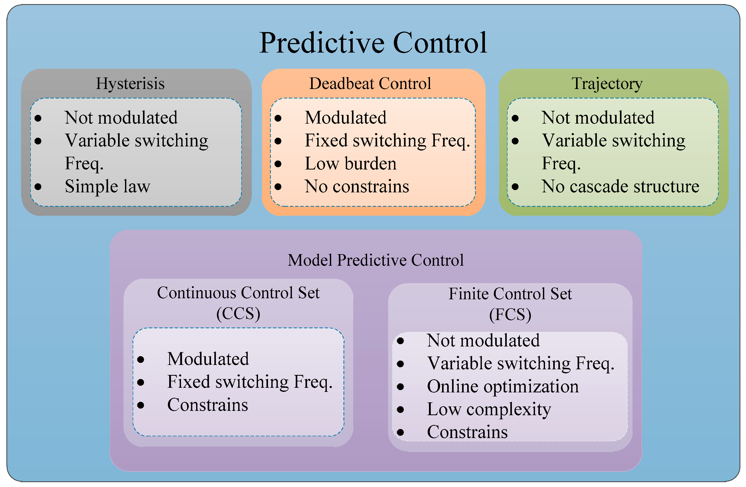
:1. Introduction
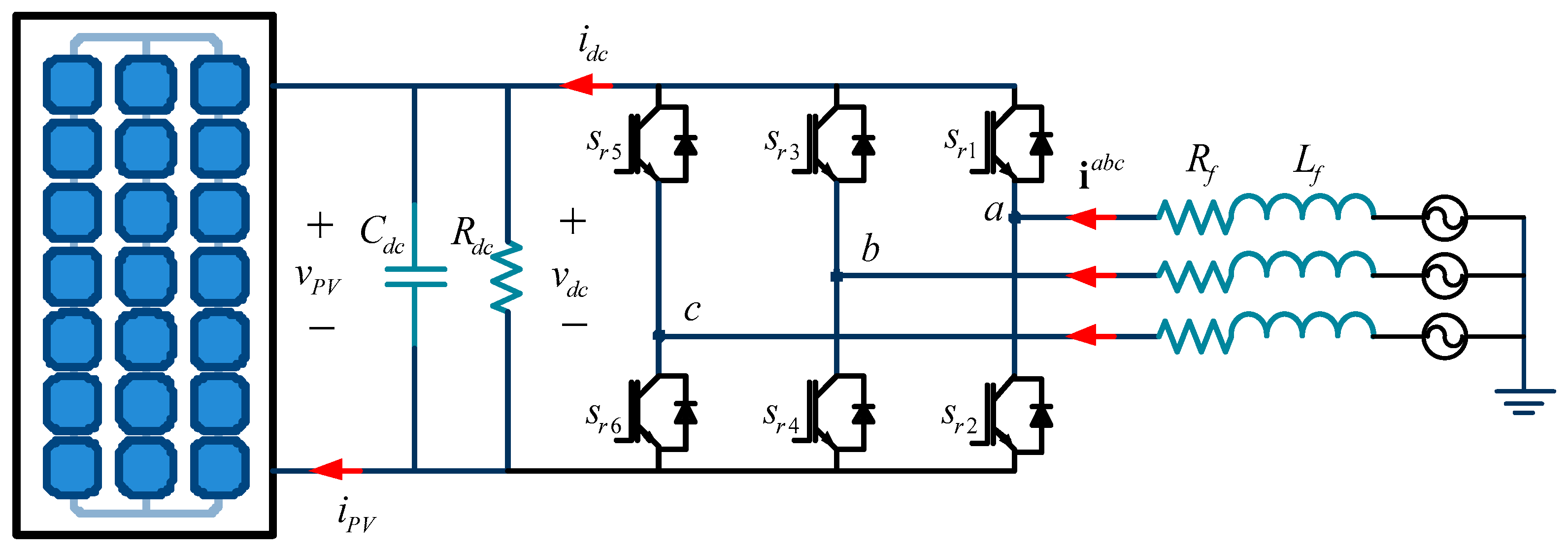
2. The Power Converter Model
2.1. The Continuous Time Converter Model
2.2. The Discrete Time Converter Model
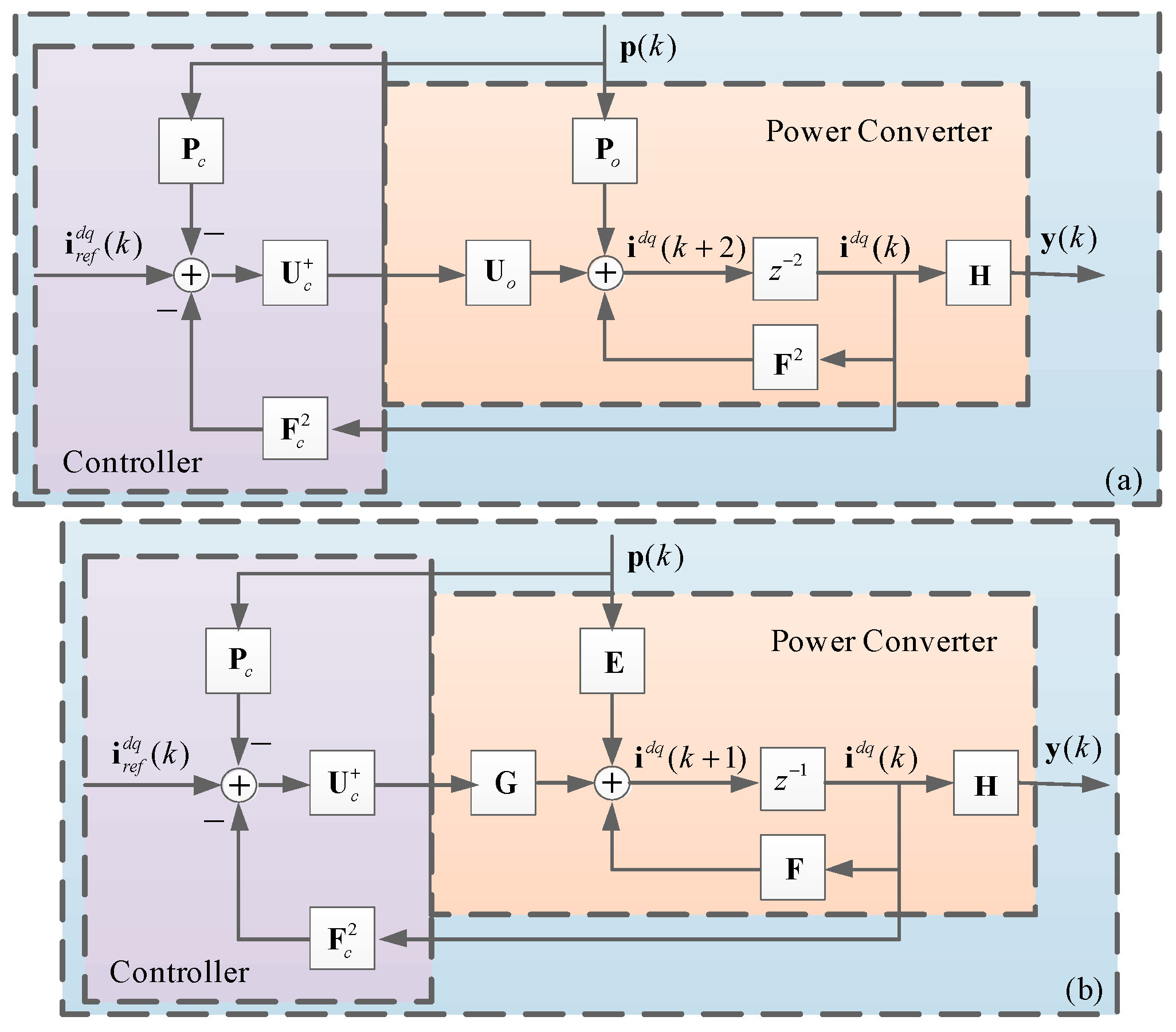
3. The Predictive Current Control Loop
3.1. Controller Output Prediction
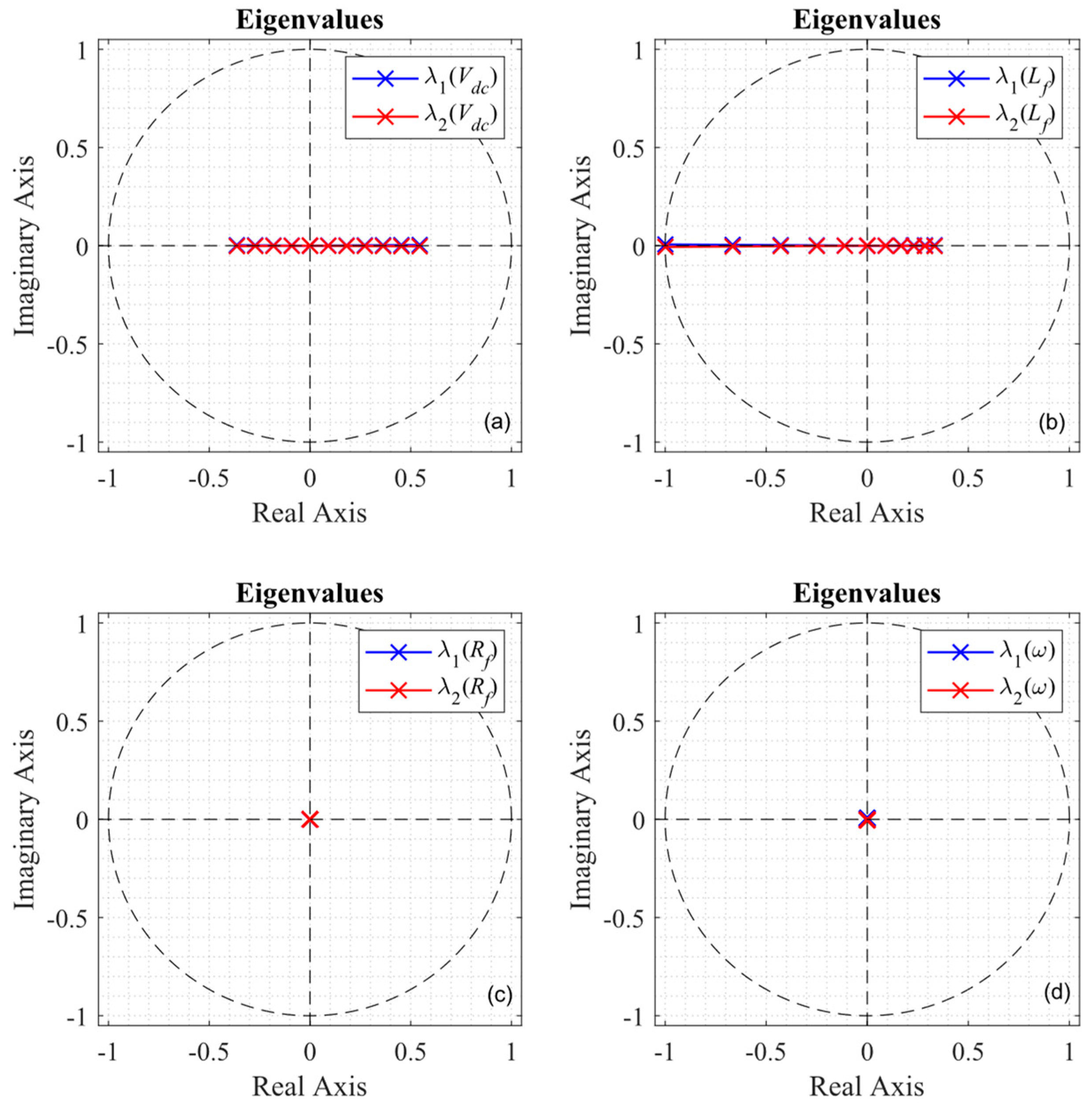
3.2. Loop Robustness and Sensibility
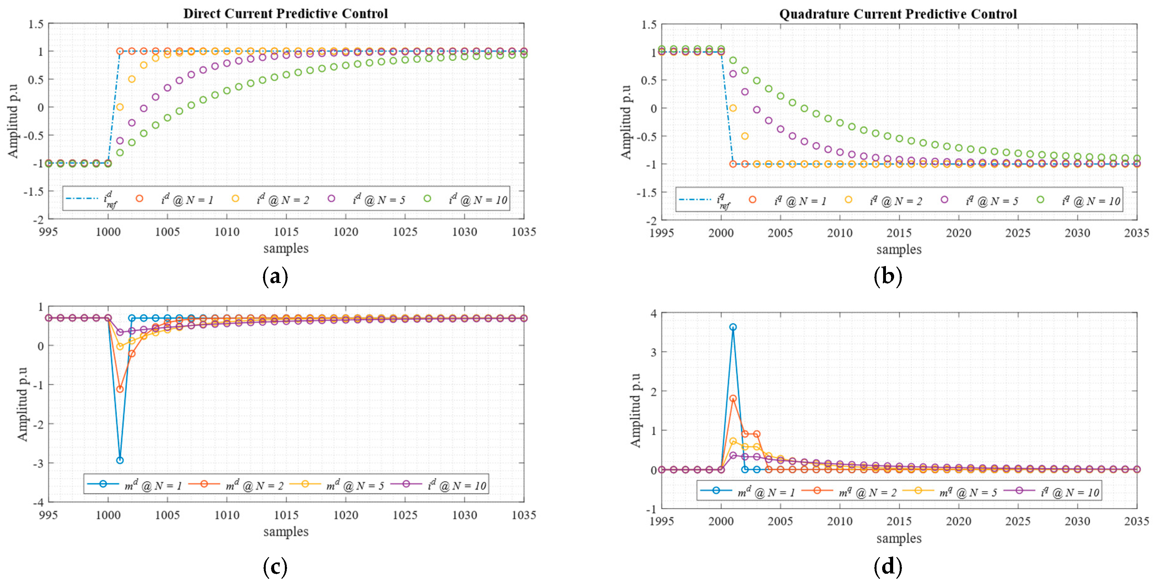
3.3. Steady-State Response
3.4. Lyapunov Stability Analysis
4. Integral State Feedback Support
4.1. Discrete Integration
4.2. Optimal Eigenvalue Placement
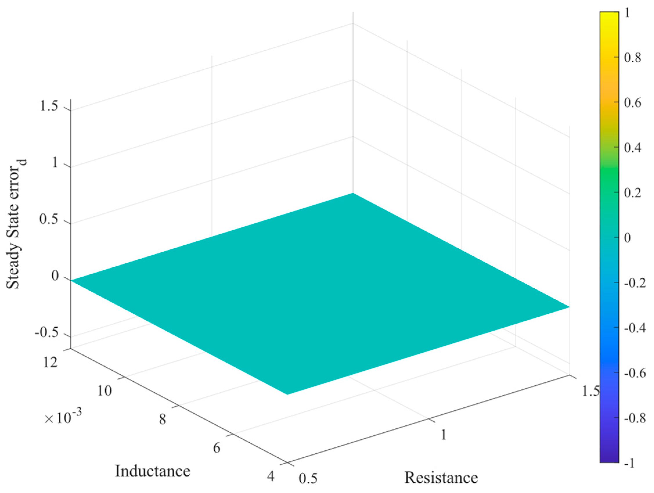
4.3. Steady-State Response
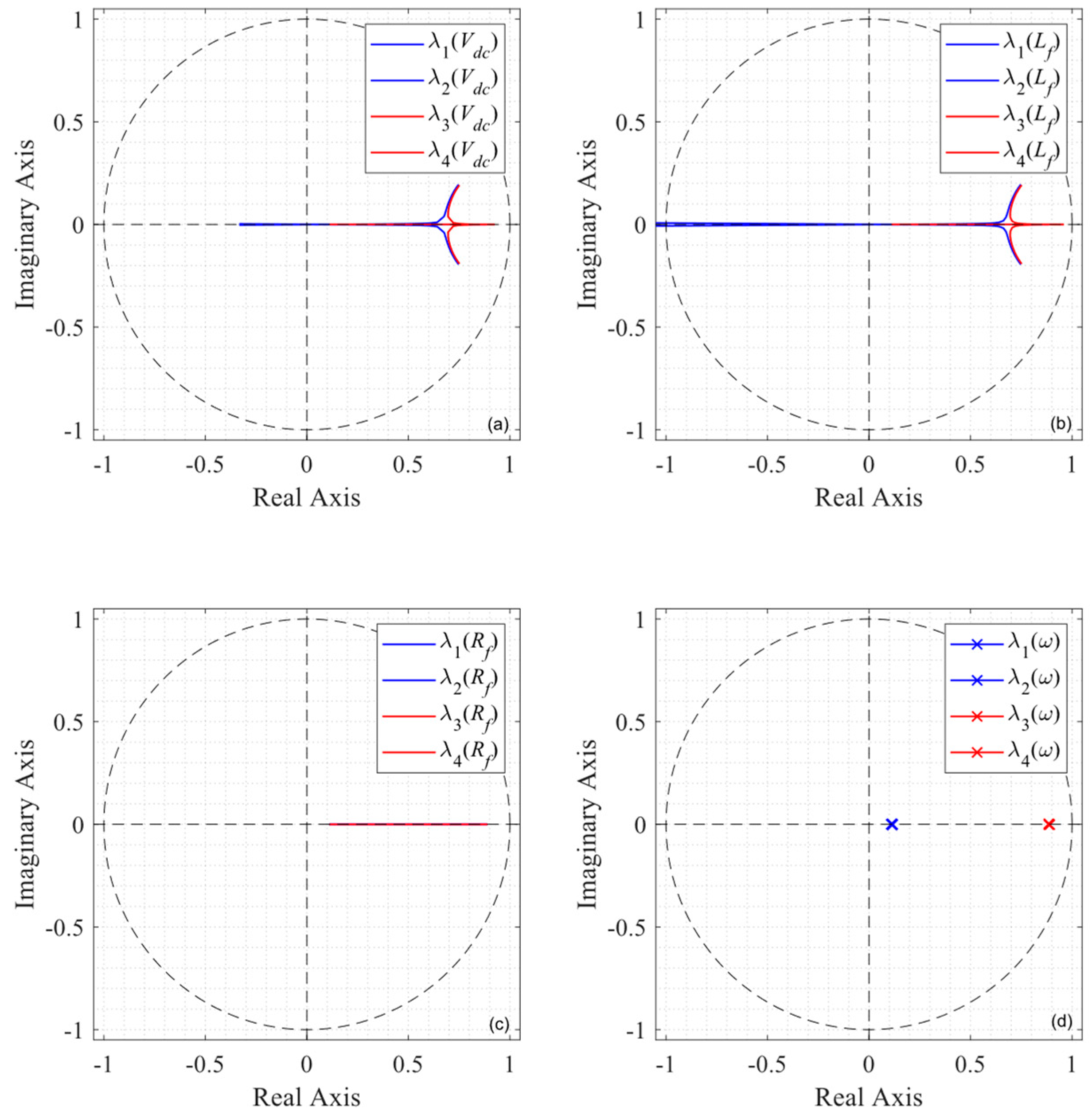
4.4. Robustness and Sensitivity
5. Active and Reactive Power Control Loops
5.1. Plant Modeling
5.2. The DC Voltage Controller
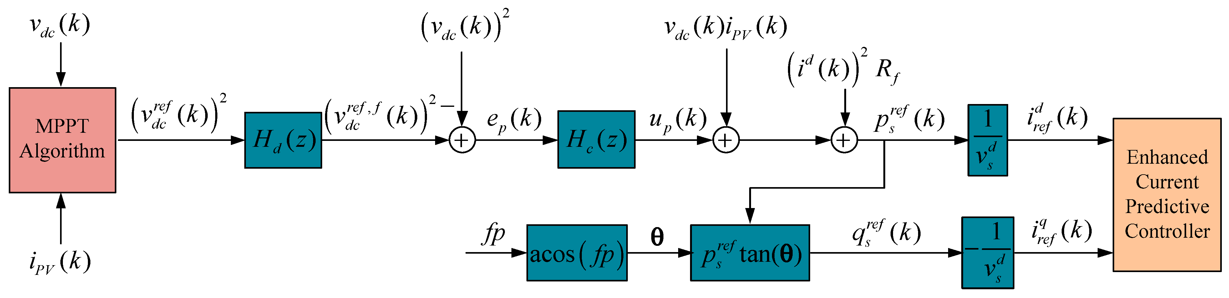
5.3. Current Reference
6. Results
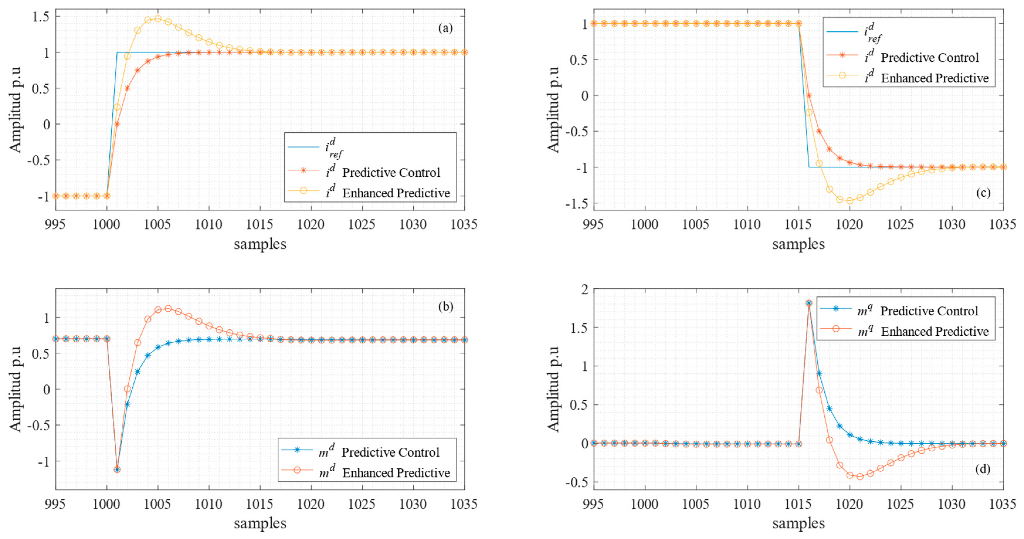
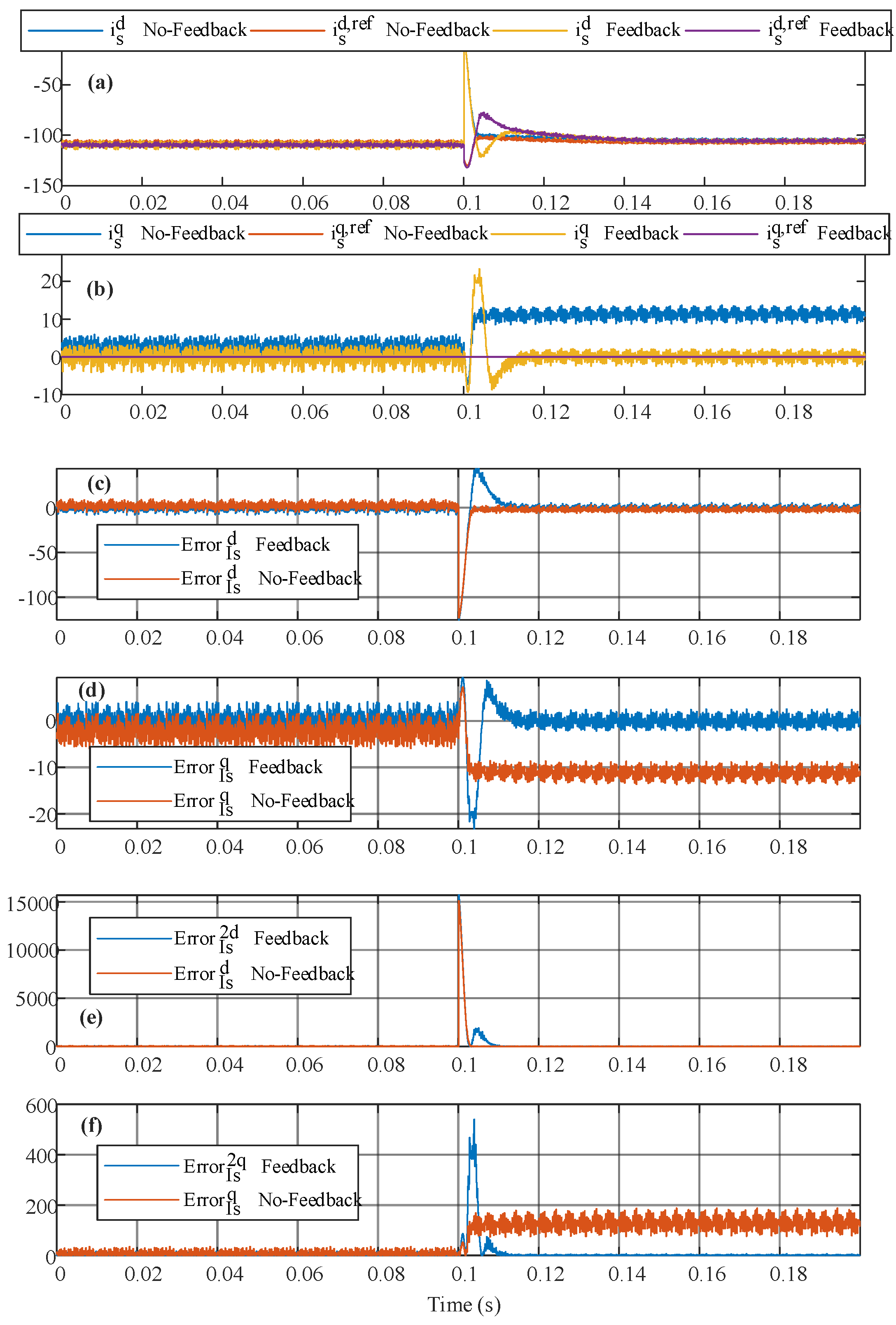
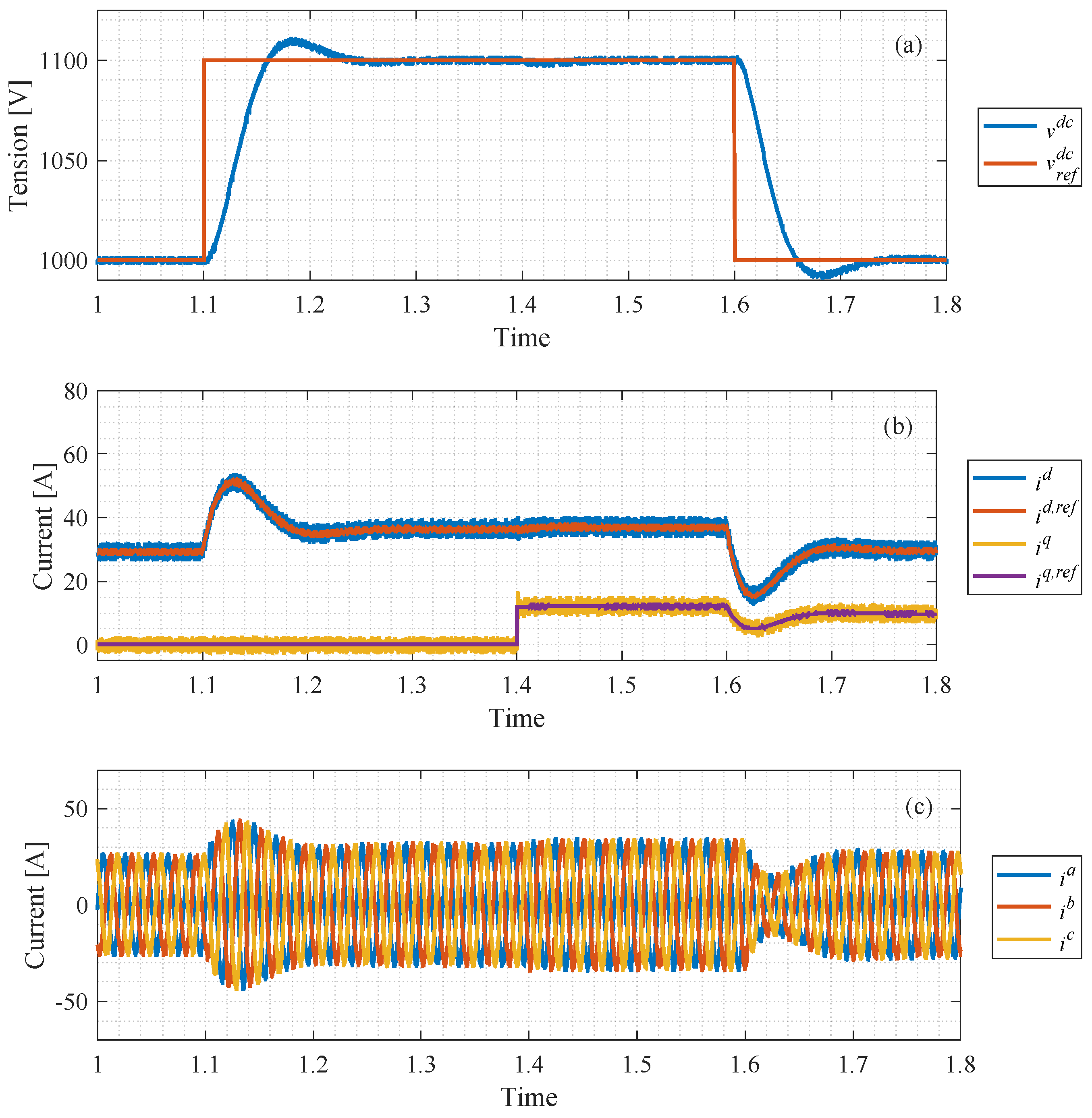
6.1. Simulations
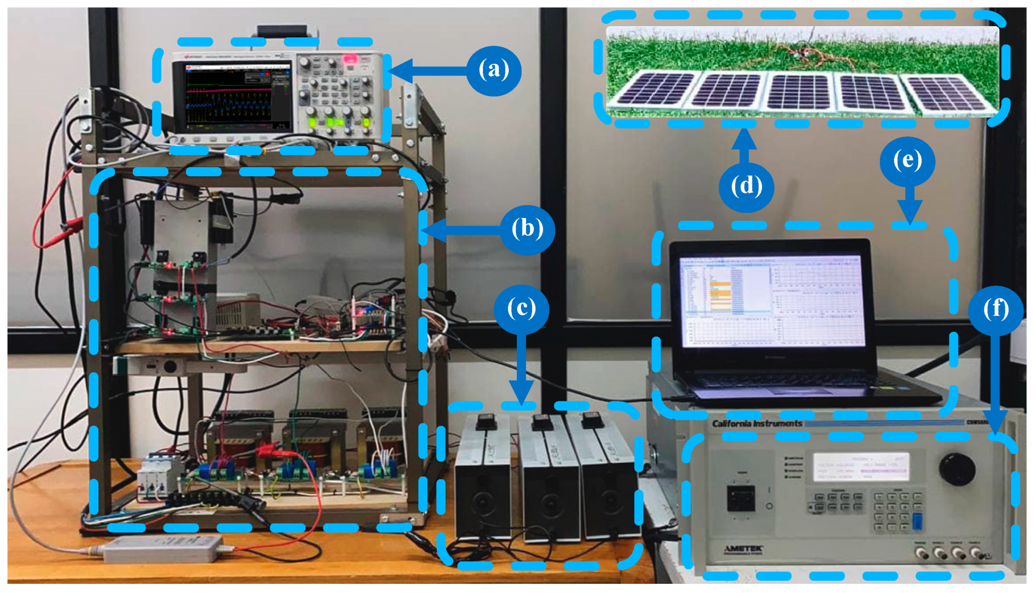
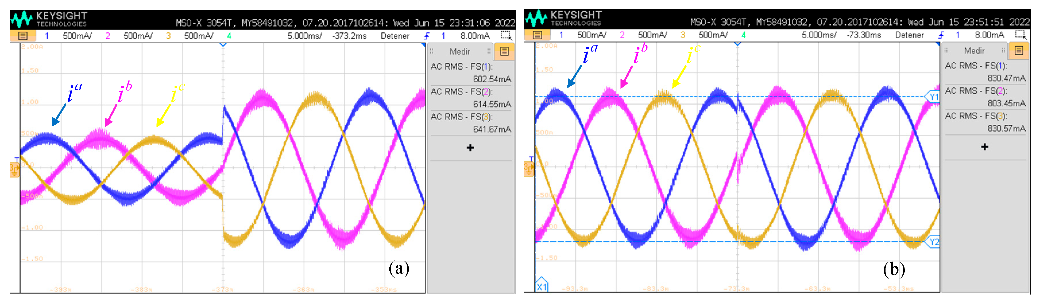
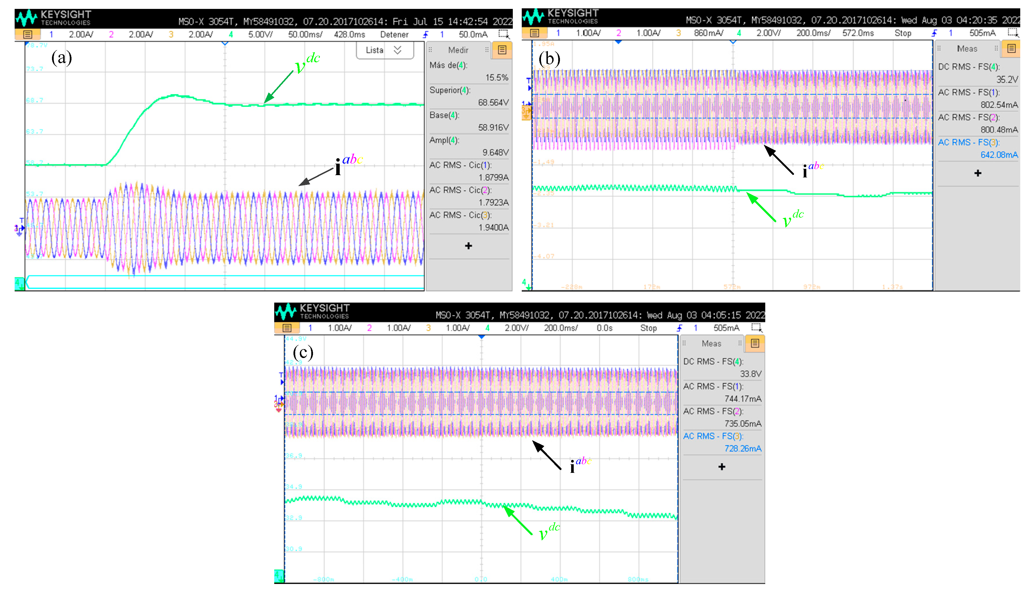
6.2. Experimental Procedure
7. Conclusions
Author Contributions
Funding
Institutional Review Board Statement
Informed Consent Statement
Data Availability Statement
Acknowledgments
Conflicts of Interest
References
- Hu, J.; Li, Z.; Zhu, J.; Guerrero, J.M. Voltage Stabilization: A Critical Step Toward High Photovoltaic Penetration. IEEE Ind. Electron. Mag. 2019, 13, 17–30. [Google Scholar] [CrossRef]
- De-Jesús-Grullón, R.E.; Batista Jorge, R.O.; Espinal Serrata, A.; Bueno Díaz, J.E.; Pichardo Estévez, J.J.; Guerrero-Rodríguez, N.F. Modeling and Simulation of Distribution Networks with High Renewable Penetration in Open-Source Software: QGIS and OpenDSS. Energies 2024, 17, 2925. [Google Scholar] [CrossRef]
- Carrasco, J.M.; Franquelo, L.G.; Bialasiewicz, J.T.; Galvan, E.; PortilloGuisado, R.C.; Prats, M.A.M.; Leon, J.I.; Moreno-Alfonso, N. Power-Electronic Systems for the Grid Integration of Renewable Energy Sources: A Survey. IEEE Trans. Ind. Electron. 2006, 53, 1002–1016. [Google Scholar] [CrossRef]
- Alqahtani, S.; Shaher, A.; Garada, A.; Cipcigan, L. Impact of the High Penetration of Renewable Energy Sources on the Frequency Stability of the Saudi Grid. Electronics 2023, 12, 1470. [Google Scholar] [CrossRef]
- Rodrigues, N.; Cunha, J.; Monteiro, V.; Afonso, J.L. Development and Experimental Validation of a Reduced-Scale Single-Phase Modular Multilevel Converter Applied to a Railway Static Converter. Electronics 2023, 12, 1367. [Google Scholar] [CrossRef]
- Guarderas, G.; Frances, A.; Ramirez, D.; Asensi, R.; Uceda, J. Blackbox Large-Signal Modeling of Grid-Connected DC-AC Electronic Power Converters. Energies 2019, 12, 989. [Google Scholar] [CrossRef]
- Ma, D.; Li, W. Wind-Storage Combined Virtual Inertial Control Based on Quantization and Regulation Decoupling of Active Power Increments. Energies 2022, 15, 5184. [Google Scholar] [CrossRef]
- Alam, M.S.; Almehizia, A.A.; Al-Ismail, F.S.; Hossain, M.A.; Islam, M.A.; Shafiullah, M.; Ullah, A. Frequency Stabilization of AC Microgrid Clusters: An Efficient Fractional Order Supercapacitor Controller Approach. Energies 2022, 15, 5179. [Google Scholar] [CrossRef]
- Wang, X.; Wei, X.; Meng, Y. Experiment on Grid-Connection Process of Wind Turbines in Fractional Frequency Wind Power System. IEEE Trans. Energy Convers. 2015, 30, 22–31. [Google Scholar] [CrossRef]
- Barrera-Cardenas, R.; Molinas, M. Comparative Study of Wind Turbine Power Converters Based on Medium-Frequency AC-Link for Offshore DC-Grids. IEEE J. Emerg. Sel. Top. Power Electron. 2015, 3, 525–541. [Google Scholar] [CrossRef]
- Silva, J.J.; Espinoza, J.R.; Rohten, J.A.; Pulido, E.S.; Villarroel, F.A.; Torres, M.A.; Reyes, M.A. MPC Algorithm With Reduced Computational Burden and Fixed Switching Spectrum for a Multilevel Inverter in a Photovoltaic System. IEEE Access 2020, 8, 77405–77414. [Google Scholar] [CrossRef]
- Jaen-Cuellar, A.Y.; Elvira-Ortiz, D.A.; Osornio-Rios, R.A.; Antonino-Daviu, J.A. Advances in Fault Condition Monitoring for Solar Photovoltaic and Wind Turbine Energy Generation: A Review. Energies 2022, 15, 5404. [Google Scholar] [CrossRef]
- Dambrosio, L.; Manzari, S.P. Multi-Objective Sensitivity Analysis of a Wind Turbine Equipped with a Pumped Hydro Storage System Using a Reversible Hydraulic Machine. Energies 2024, 17, 4078. [Google Scholar] [CrossRef]
- Cavdar, M.; Ozcira Ozkilic, S. A Novel Linear-Based Closed-Loop Control and Analysis of Solid-State Transformer. Electronics 2024, 13, 3253. [Google Scholar] [CrossRef]
- Chen, Z.; Guerrero, J.M.; Blaabjerg, F. A Review of the State of the Art of Power Electronics for Wind Turbines. IEEE Trans. Power Electron. 2009, 24, 1859–1875. [Google Scholar] [CrossRef]
- Aliaga, R.; Rivera, M.; Wheeler, P.; Munoz, J.; Rohten, J.; Sebaaly, F.; Villalon, A.; Trentin, A. Implementation of Exact Linearization Technique for Modeling and Control of DC/DC Converters in Rural PV Microgrid Application. IEEE Access 2022, 10, 56925–56936. [Google Scholar] [CrossRef]
- Espinoza Trejo, D.R.; Taheri, S.; Saavedra, J.L.; Vazquez, P.; De Angelo, C.H.; Pecina-Sanchez, J.A. Nonlinear Control and Internal Stability Analysis of Series-Connected Boost DC/DC Converters in PV Systems With Distributed MPPT. IEEE J. Photovolt. 2021, 11, 504–512. [Google Scholar] [CrossRef]
- Rohten, J.A.; Silva, J.J.; Munoz, J.A.; Villarroel, F.A.; Dewar, D.N.; Rivera, M.E.; Espinoza, J.R. A Simple Self-Tuning Resonant Control Approach for Power Converters Connected to Micro-Grids With Distorted Voltage Conditions. IEEE Access 2020, 8, 216018–216028. [Google Scholar] [CrossRef]
- Rodriguez, J.; Pontt, J.; Silva, C.A.; Correa, P.; Lezana, P.; Cortes, P.; Ammann, U. Predictive Current Control of a Voltage Source Inverter. IEEE Trans. Ind. Electron. 2007, 54, 495–503. [Google Scholar] [CrossRef]
- Rodriguez, J.; Cortes, P. Predictive Control of Power Converters and Electrical Drives; John Wiley & Sons, Ltd.: Chichester, UK, 2012; ISBN 9781119941446. [Google Scholar]
- Cortes, P.; Ortiz, G.; Yuz, J.I.; Rodriguez, J.; Vazquez, S.; Franquelo, L.G. Model Predictive Control of an Inverter With Output $LC$ Filter for UPS Applications. IEEE Trans. Ind. Electron. 2009, 56, 1875–1883. [Google Scholar] [CrossRef]
- Comarella, B.V.; Carletti, D.; Yahyaoui, I.; Encarnação, L.F. Theoretical and Experimental Comparative Analysis of Finite Control Set Model Predictive Control Strategies. Electronics 2023, 12, 1482. [Google Scholar] [CrossRef]
- Rohten, J.A.; Dewar, D.N.; Zanchetta, P.; Formentini, A.; Muñoz, J.A.; Baier, C.R.; Silva, J.J. Multivariable Deadbeat Control of Power Electronics Converters with Fast Dynamic Response and Fixed Switching Frequency. Energies 2021, 14, 313. [Google Scholar] [CrossRef]
- Dan, H.; Zeng, P.; Xiong, W.; Wen, M.; Su, M.; Rivera, M. Model Predictive Control-Based Direct Torque Control for Matrix Converter-Fed Induction Motor with Reduced Torque Ripple. CES Trans. Electr. Mach. Syst. 2021, 5, 90–99. [Google Scholar] [CrossRef]
- Li, X.; Wang, Y.; Guo, X.; Cui, X.; Zhang, S.; Li, Y. An Improved Model-Free Current Predictive Control Method for SPMSM Drives. IEEE Access 2021, 9, 134672–134681. [Google Scholar] [CrossRef]
- Prieto Cerón, C.E.; Normandia Lourenço, L.F.; Solís-Chaves, J.S.; Sguarezi Filho, A.J. A Generalized Predictive Controller for a Wind Turbine Providing Frequency Support for a Microgrid. Energies 2022, 15, 2562. [Google Scholar] [CrossRef]
- Panten, N.; Hoffmann, N.; Fuchs, F.W. Finite Control Set Model Predictive Current Control for Grid-Connected Voltage-Source Converters With LCL Filters: A Study Based on Different State Feedbacks. IEEE Trans. Power Electron. 2016, 31, 5189–5200. [Google Scholar] [CrossRef]
- Geyer, T. Model Predictive Direct Torque Control: Derivation and Analysis of the State-Feedback Control Law. IEEE Trans. Ind. Appl. 2013, 49, 2146–2157. [Google Scholar] [CrossRef]
- Hu, J.; Ding, B. Output Feedback MPC for Nonlinear System in Large Operation Range. IEEE Trans. Autom. Control 2023, 68, 7903–7910. [Google Scholar] [CrossRef]
- Li, H.; Lin, J.; Lu, Z. Three Vectors Model Predictive Torque Control Without Weighting Factor Based on Electromagnetic Torque Feedback Compensation. Energies 2019, 12, 1393. [Google Scholar] [CrossRef]
- Wang, Z.; Yin, Z.; Yu, F.; Long, Y.; Ni, S.; Gao, P. A Novel Finite-Set Ultra-Local Model-Based Predictive Current Control for AC/DC Converters of Direct-Driven Wind Power Generation with Enhanced Steady-State Performance. Electronics 2024, 13, 3302. [Google Scholar] [CrossRef]
- Zhong, Q.; Wu, K.; Luo, N.; Chen, Z.; Shi, J. Inverse Park Transformation PLL for VSC-HVDC under Unbalanced Voltage Condition. In Proceedings of the 2022 6th International Conference on Smart Grid and Smart Cities (ICSGSC), Chengdu, China, 22–24 October 2022; IEEE: Piscataway, NJ, USA; pp. 98–102. [Google Scholar]
- Barhoumi, L.; Bemri, H.; Soudani, D. Discretization of Uncertain Linears Systems with Time Delay via Euler’s and Tustin’s Approximations. In Proceedings of the 2016 4th International Conference on Control Engineering & Information Technology (CEIT), Hammamet, Tunisia, 16–18 December 2016; IEEE: Piscataway, NJ, USA; pp. 1–6. [Google Scholar]
- Zhang, H.; Prempain, E. A Non-Linear Offset-Free Model Predictive Control Design Approach. Actuators 2024, 13, 322. [Google Scholar] [CrossRef]
- Chen, D.; Liu, X.; Shi, K.; Yang, J.; Tashi, N. A Necessary and Sufficient Stability Condition of Discrete-Time Monotone Systems: A Max-Separable Lyapunov Function Method. IEEE Trans. Circuits Syst. II Express Briefs 2024, 71, 276–280. [Google Scholar] [CrossRef]
- Li, H.; Ren, F.; Shang, J.; Zhang, B.; Lu, J.; Qi, H. A Novel Large-Signal Stability Analysis Approach Based on Semi-Tensor Product of Matrices with Lyapunov Stability Theorem for DC-DC Converters. In Proceedings of the 2016 IEEE Energy Conversion Congress and Exposition (ECCE), Milwaukee, WI, USA, 18–22 September 2016; IEEE: Piscataway, NJ, USA; pp. 1–5. [Google Scholar]
- Rohten, J.; Villarroel, F.; Pulido, E.; Muñoz, J.; Silva, J.; Perez, M. Stability Analysis of Two Power Converters Control Algorithms Connected to Micro-Grids with Wide Frequency Variation. Sensors 2022, 22, 7078. [Google Scholar] [CrossRef] [PubMed]


| Parameter | Value | |
|---|---|---|
| Rf (line resistance) | 1 | Ω |
| Lf (line inductance) | 10 | mH |
| Vs (RMS grid voltage) | 220 | V |
| ω (angular frequency) | 2π50 | rad/s |
| Gac (converter gain) | 0.5 | p.u. |
| Vdc (DC voltage) | 1000 | V |
| Ts (sampling period) | 100 | µs |
| Squared Mean Error | Type of Control | Parameter Deviations? | Values |
|---|---|---|---|
| No Feedback | Yes | 8.0001 | |
| No Feedback | Yes | 127.9266 | |
| Feedback | Yes | 4.0722 | |
| Feedback | Yes | 1.3007 | |
| No Feedback | No | 17.4967 | |
| No Feedback | No | 9.9013 | |
| Feedback | No | 12.9180 | |
| Feedback | No | 3.7939 |
Disclaimer/Publisher’s Note: The statements, opinions and data contained in all publications are solely those of the individual author(s) and contributor(s) and not of MDPI and/or the editor(s). MDPI and/or the editor(s) disclaim responsibility for any injury to people or property resulting from any ideas, methods, instructions or products referred to in the content. |
© 2024 by the authors. Licensee MDPI, Basel, Switzerland. This article is an open access article distributed under the terms and conditions of the Creative Commons Attribution (CC BY) license (https://creativecommons.org/licenses/by/4.0/).
Share and Cite
Andreu, M.; Rohten, J.; Espinoza, J.; Silva, J.; Pulido, E.; Leon, L. Enhanced Model Predictive Control Using State Variable Feedback for Steady-State Error Cancellation. Sensors 2024, 24, 5869. https://doi.org/10.3390/s24185869
Andreu M, Rohten J, Espinoza J, Silva J, Pulido E, Leon L. Enhanced Model Predictive Control Using State Variable Feedback for Steady-State Error Cancellation. Sensors. 2024; 24(18):5869. https://doi.org/10.3390/s24185869
Chicago/Turabian StyleAndreu, Marcos, Jaime Rohten, José Espinoza, José Silva, Esteban Pulido, and Lesyani Leon. 2024. "Enhanced Model Predictive Control Using State Variable Feedback for Steady-State Error Cancellation" Sensors 24, no. 18: 5869. https://doi.org/10.3390/s24185869