
CFD Analyses of Density Gradients under Conditions of Supersonic Flow at Low Pressures

 , , , , and
Abstract
:1. Introduction
2. Methodology
- Accurate capture of shock and contact discontinuities.
- Entropy-conserving solution capabilities.
- Suppression of the carbuncle phenomenon, a common numerical instability associated with low-dissipative shock-capturing schemes.
- Robust accuracy and convergence across a wide Mach number range.
3. Results
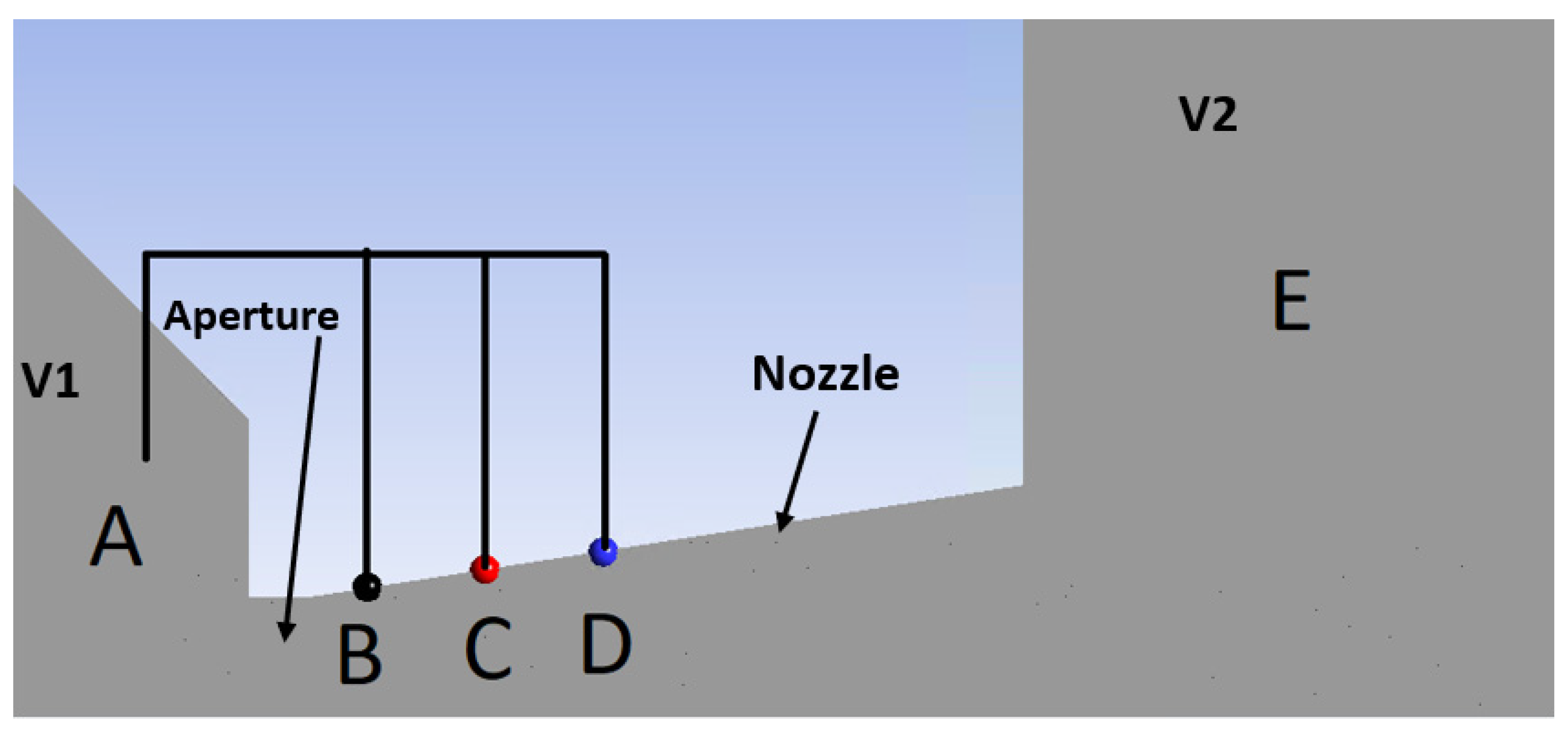
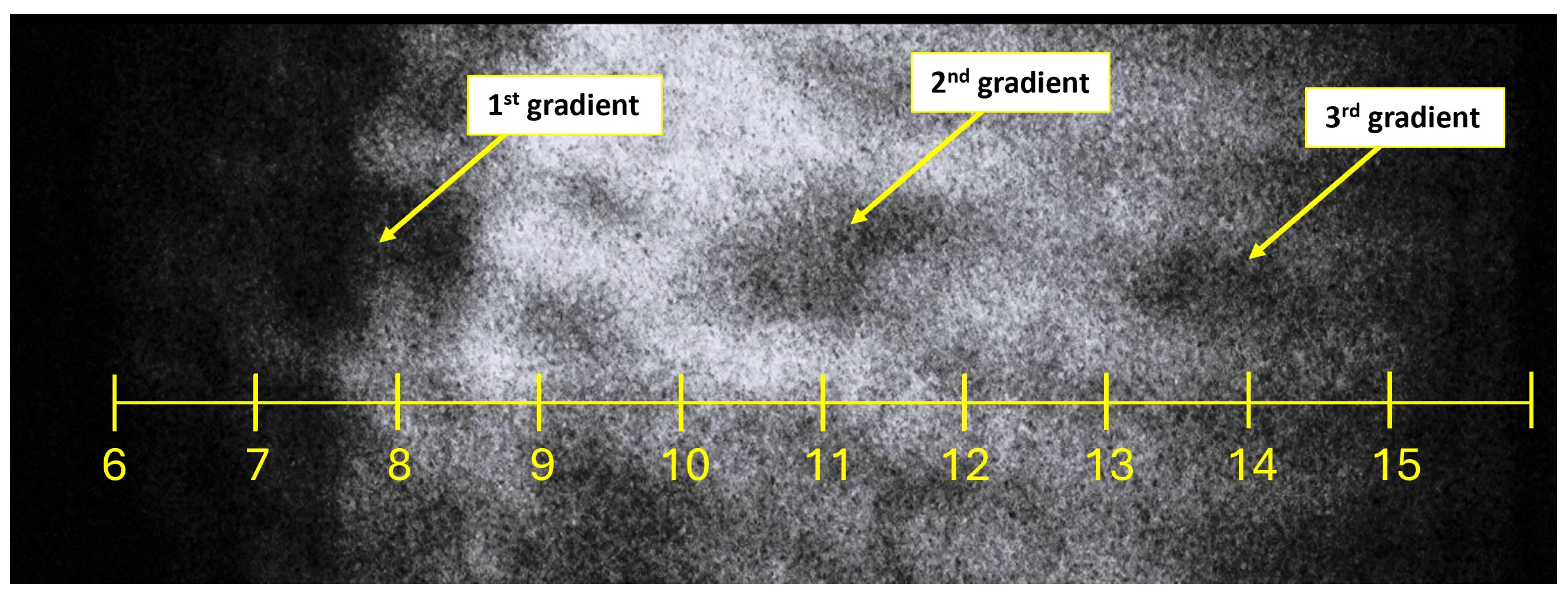
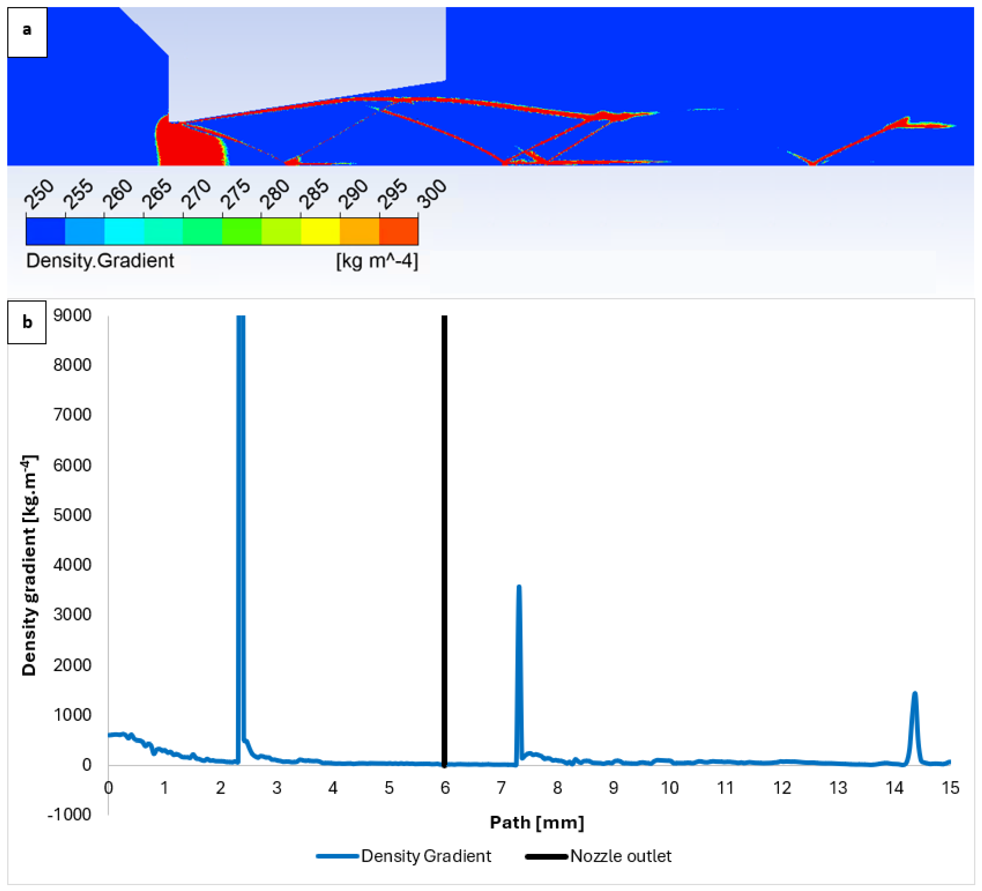
3.1. Comparison of Experiment and CFD Simulation
- The differential pressure between points A and B was measured to be 74,400 Pa using a DPS 300 sensor with a range of 100 kPa and an accuracy of ±1% FSO BFSL (over the entire range fitted with a linear curve).
- The differential pressure between points B and C was measured to be 8500 Pa using a DPS 300 sensor with a range of 25 kPa and an accuracy of ±1% FSO BFSL (over the entire range fitted with a linear curve).
- The differential pressure between points C and D was measured to be 4500 Pa using a DPS 300 sensor with a range of 4 kPa and an accuracy of ±1% FSO BFSL (over the entire range fitted with a linear curve).
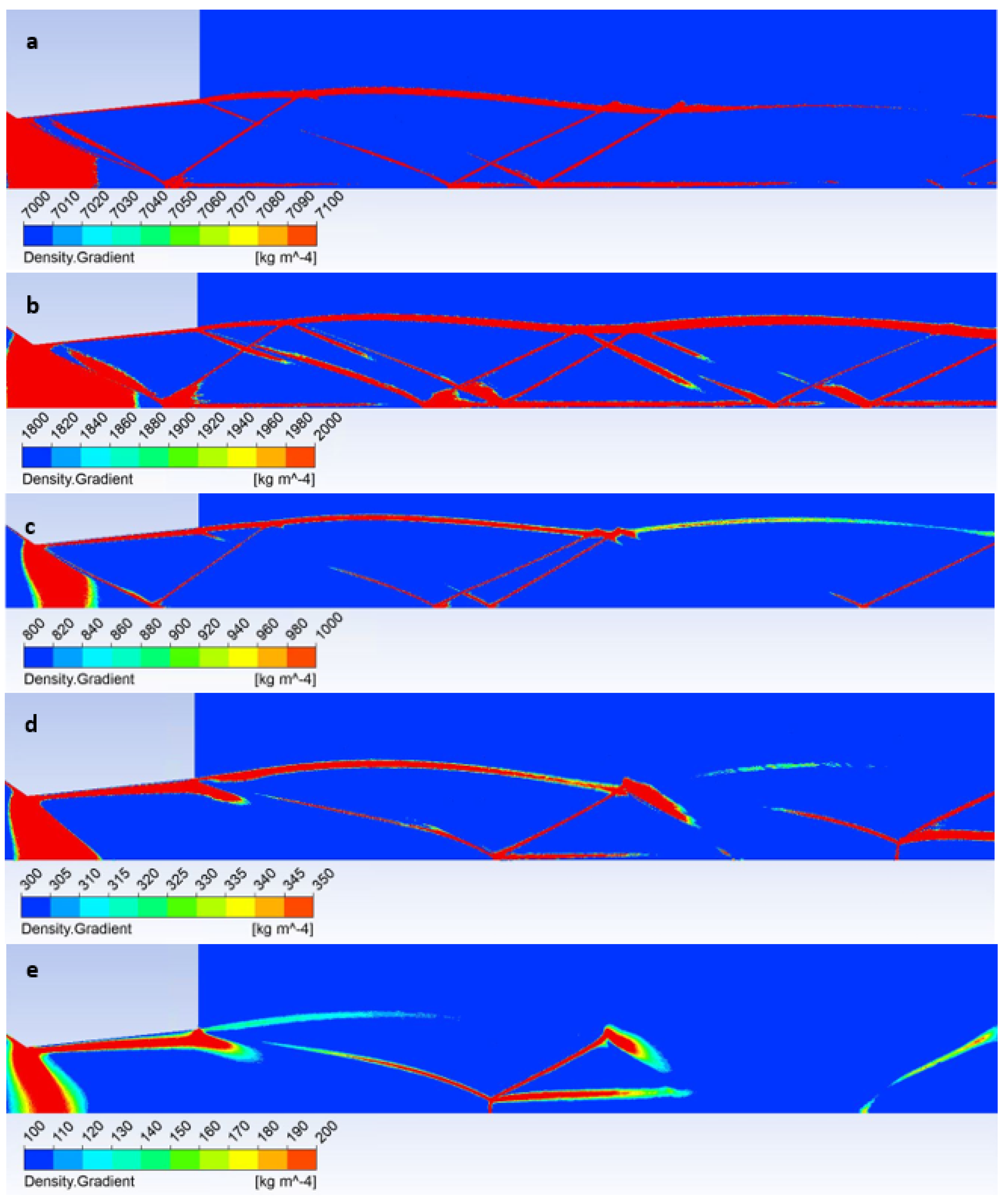
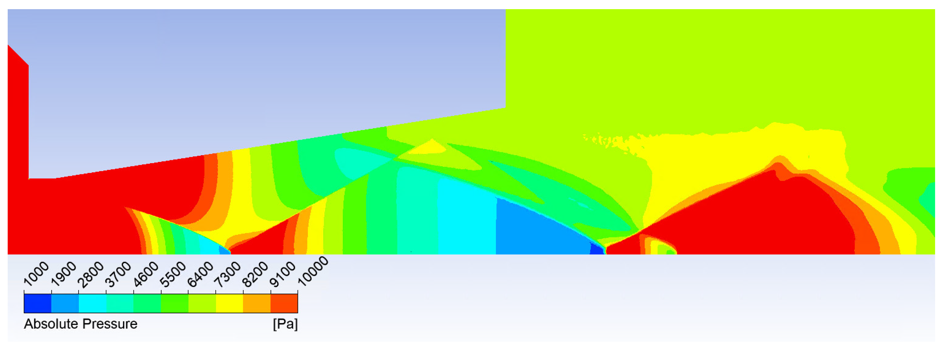
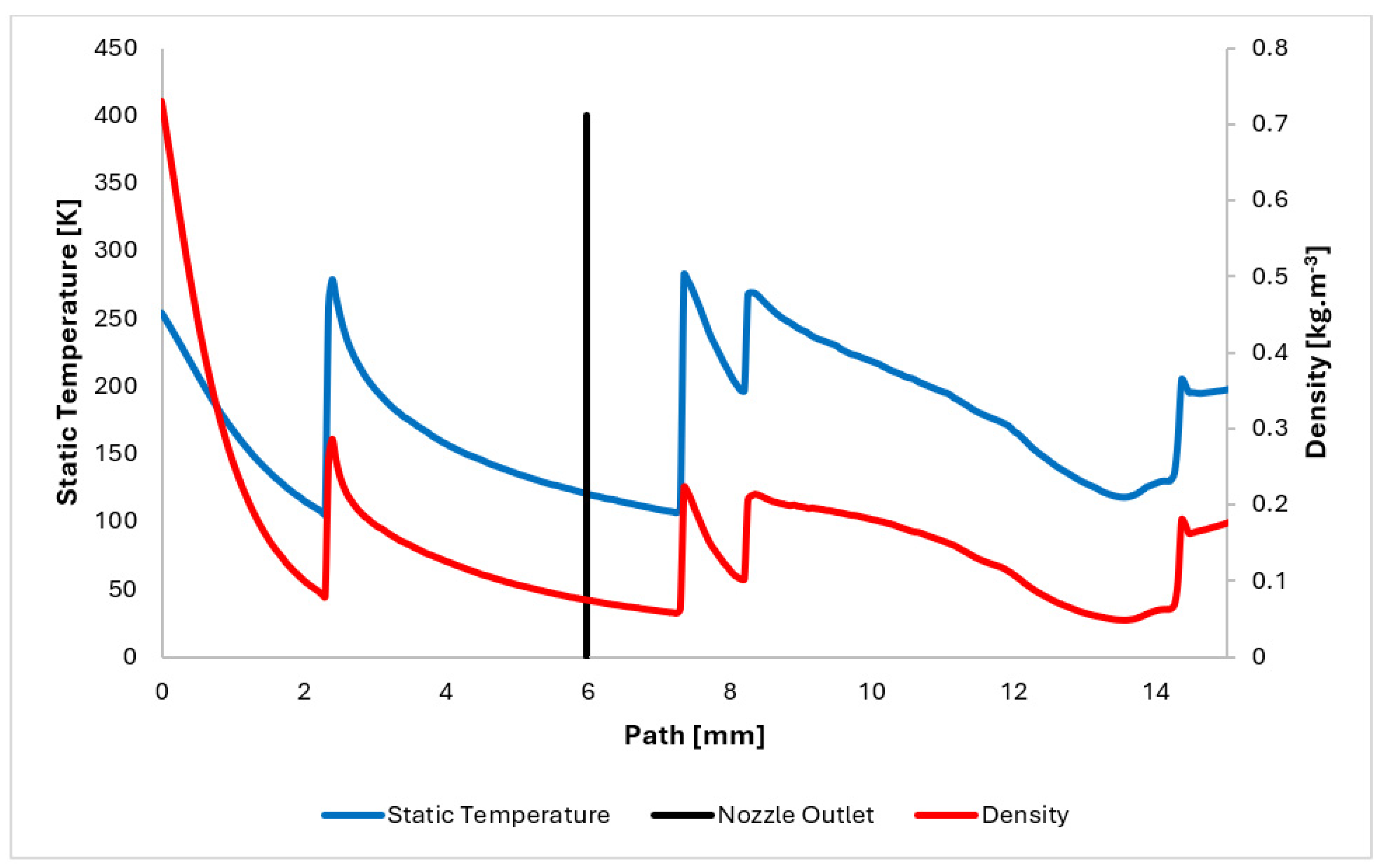
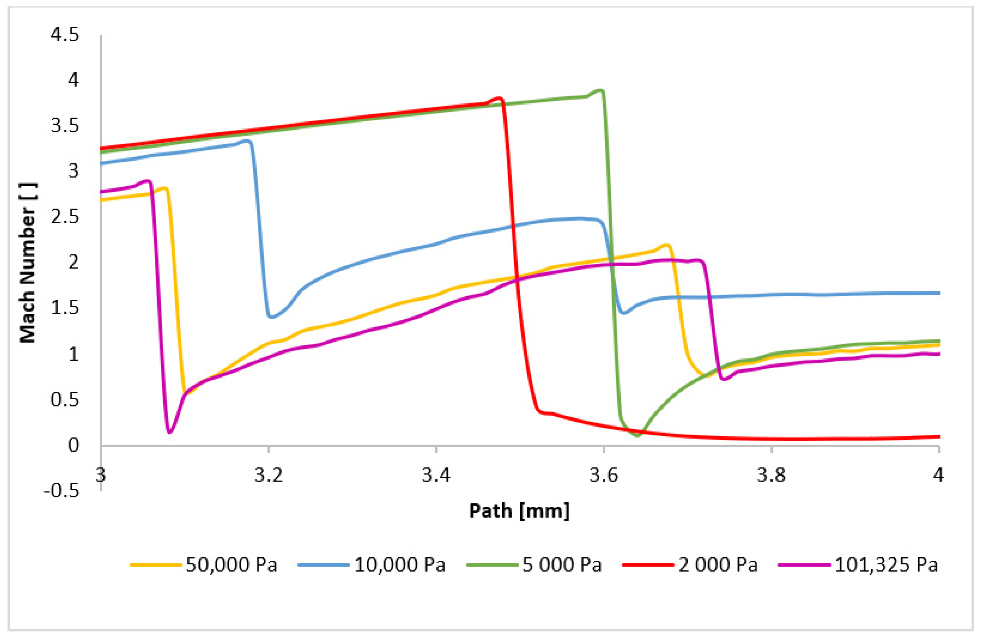
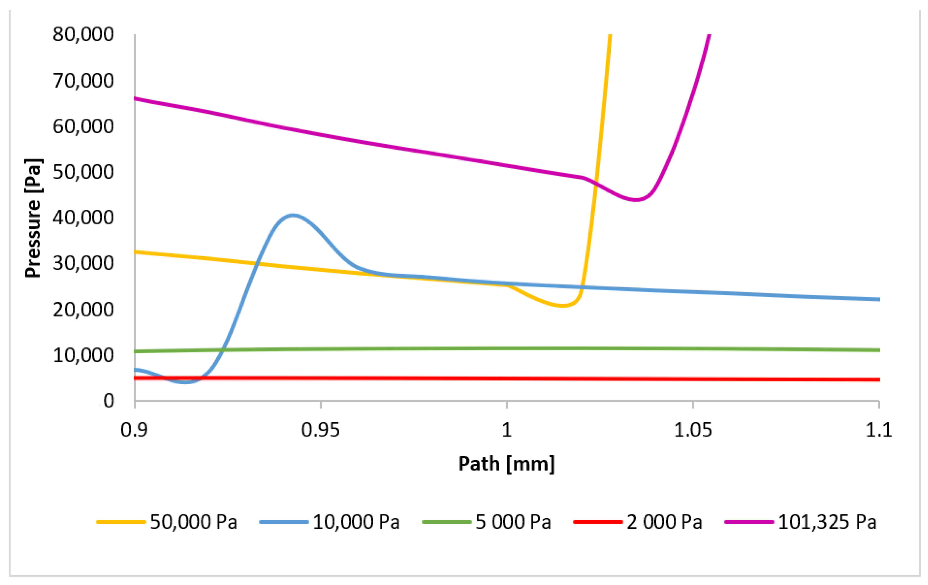
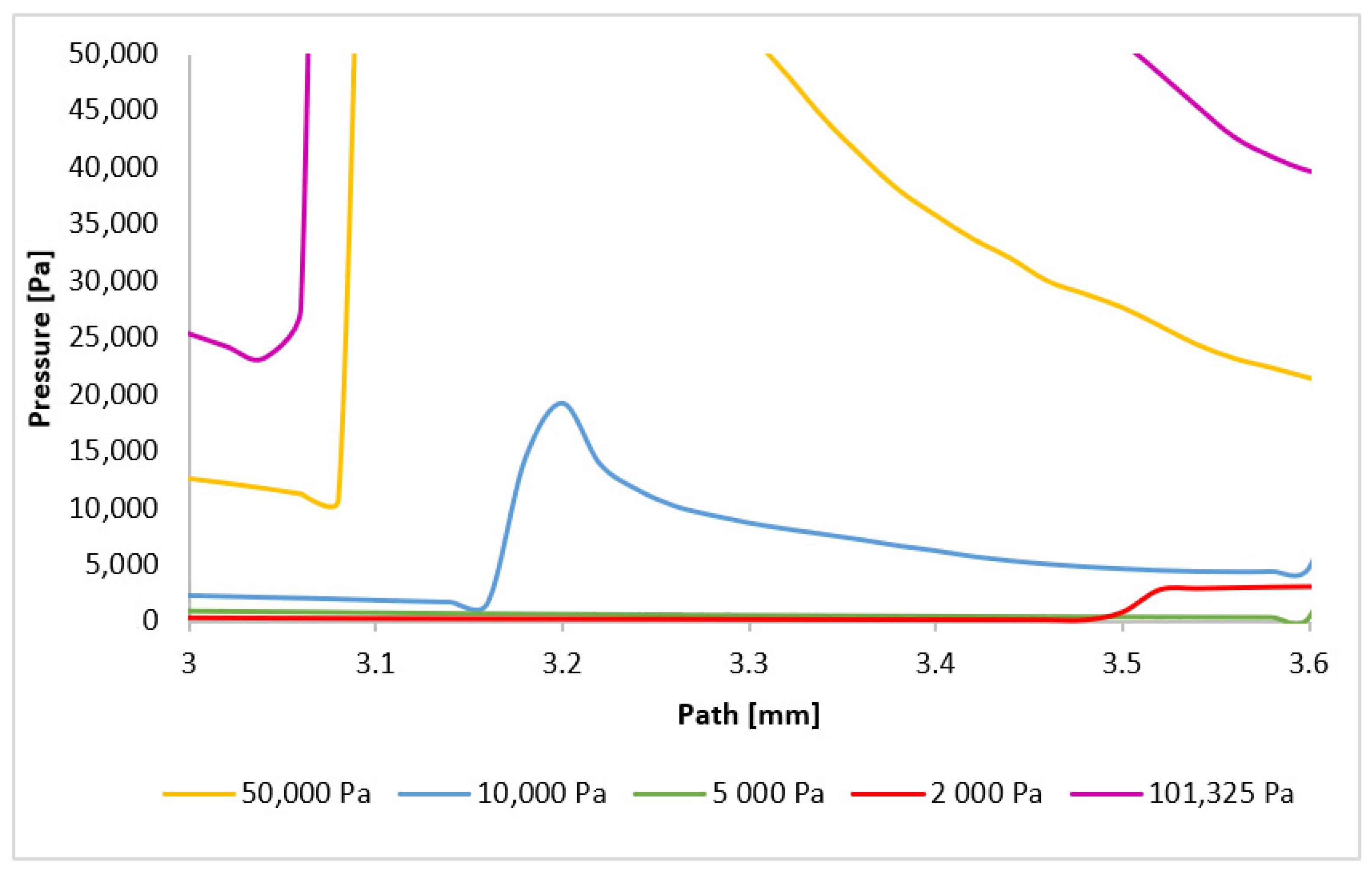
3.2. CFD Analyses of the Influence of the Pressure Magnitude on the Shock Wave Location
4. Conclusions
Author Contributions
Funding
Institutional Review Board Statement
Informed Consent Statement
Data Availability Statement
Acknowledgments
Conflicts of Interest
Appendix A


References
- Neděla, V.; Tihlaříková, E.; Maxa, J.; Imrichová, K.; Bučko, M.; Gemeiner, P. Simulation-based optimisation of thermodynamic conditions in the ESEM for dynamical in-situ study of spherical polyelectrolyte complex particles in their native state. Ultramicroscopy 2020, 211, 112954. [Google Scholar] [CrossRef] [PubMed]
- Vetráková, Ľ.; Neděla, V.; Runštuk, J.; Heger, D. The morphology of ice and liquid brine in an environmental scanning electron microscope: A study of the freezing methods. Cryosphere 2019, 13, 2385–2405. [Google Scholar] [CrossRef]
- Đorđević, B.; Neděla, V.; Tihlaříková, E.; Trojan, V.; Havel, L. Effects of copper and arsenic stress on the development of Norway spruce somatic embryos and their visualization with the environmental scanning electron microscope. New Biotechnol. 2019, 48, 35–43. [Google Scholar] [CrossRef] [PubMed]
- Imrichová, K.; Veselý, L.; Gasser, T.M.; Loerting, T.; Neděla, V.; Heger, D. Vitrification and increase of basicity in between ice Ih crystals in rapidly frozen dilute NaCl aqueous solutions. J. Chem. Phys. 2019, 151, 014503. [Google Scholar] [CrossRef] [PubMed]
- Neděla, V.; Hřib, J.; Vooková, B. Imaging of early conifer embryogenic tissues with the environmental scanning electron microscope. Biol. Plant. 2012, 56, 595–598. [Google Scholar] [CrossRef]
- Maxa, J.; Neděla, V. The impact of critical flow on the primary electron beam passage through differentially pumped chamber. Adv. Mil. Technol. 2011, 6, 39–46. [Google Scholar]
- Ritscher, A.; Schmetterer, C.; Ipser, H. Pressure dependence of the tin–phosphorus phase diagram. Monatsh. Chem. 2012, 143, 1593–1602. [Google Scholar] [CrossRef]
- Stelate, A.; Tihlaříková, E.; Schwarzerová, K.; Neděla, V.; Petrášek, J. Correlative Light-Environmental Scanning Electron Microscopy of Plasma Membrane Efflux Carriers of Plant Hormone Auxin. Biomolecules 2021, 11, 1407. [Google Scholar]
- Schenkmayerová, A.; Bučko, M.; Gemeiner, P.; Treľová, D.; Lacík, I.; Chorvát, D.; Ačai, P.; Polakovič, M.; Lipták, L.; Rebroš, M.; et al. Physical and Bioengineering Properties of Polyvinyl Alcohol Lens-Shaped Particles Versus Spherical Polyelectrolyte Complex Microcapsules as Immobilisation Matrices for a Whole-Cell Baeyer–Villiger Monooxygenase. Appl. Biochem. Biotechnol. 2014, 174, 1834–1849. [Google Scholar] [CrossRef]
- Neděla, V.; Konvalina, I.; Oral, M.; Hudec, J. The Simulation of Energy Distribution of Electrons Detected by Segmental Ionization Detector in High Pressure Conditions of ESEM. Microsc. Microanal. 2015, 21, 264–269. [Google Scholar] [CrossRef]
- van Eck, H.J.N.; Koppers, W.R.; van Rooij, G.J.; Goedheer, W.J.; Engeln, R.; Schram, D.C.; Cardozo, N.J.L.; Kleyn, A.W. Modeling and experiments on differential pumping in linear plasma generators operating at high gas flows. J. Appl. Phys. 2009, 105, 063307. [Google Scholar] [CrossRef]
- Taylor, H.G.; Waldram, J.M. Improvements in the schlieren method. J. Sci. Instrum. 1933, 10, 378–389. [Google Scholar] [CrossRef]
- Richard, H.; Raffel, M. Principle and applications of the background oriented schlieren (BOS)method. Meas. Sci. Technol. 2001, 12, 1576. [Google Scholar] [CrossRef]
- Schradin, H. Schlieren methods and their applications. Ergeb. Exakten Naturewiss 1942, 20, 303–439. [Google Scholar]
- Danilatos, G.D. Velocity and ejector-jet assisted differential pumping: Novel design stages for environmental SEM. Micron 2012, 43, 600–611. [Google Scholar] [CrossRef]
- Danilatos, G.D. Figure of merit for environmental SEM and its implications. J. Microsc. 2011, 244, 159–169. [Google Scholar] [CrossRef]
- Danilatos, G.D. Optimum beam transfer in the environmental scanning electron microscope. J. Microsc. 2009, 234, 26–37. [Google Scholar] [CrossRef]
- Danilatos, G.D.; Rattenberger, J.; Dracopoulos, V. Beam transfer characteristics of a commercial environmental SEM and a low vacuum SEM. J. Microsc. 2011, 242, 166–180. [Google Scholar] [CrossRef]
- Xue, Z.; Zhou, L.; Liu, D. Accurate Numerical Modeling for 1D Open-Channel Flow with Varying Topography. Water 2023, 15, 2893. [Google Scholar] [CrossRef]
- Škorpík, J. Proudění plynů a par tryskami. Transform. Technol. 2006, 2, 1–20. [Google Scholar]
- Moran, M.J.; Shapiro, H.N. Fundamentals of Engineering Thermodynamics, 3rd ed.; John and Wiley and Sons: Hoboken, NJ, USA, 1998. [Google Scholar]
- Nasuti, F.; Onofri, M. Shock structure in separated nozzle flows. Shock. Waves 2008, 19, 229–237. [Google Scholar] [CrossRef]
- Gong, C.; Ou, M.; Jia, W. The effect of nozzle configuration on the evolution of jet surface structure. Results Phys. 2019, 15, 102572. [Google Scholar] [CrossRef]
- Yuan, T.-F.; Zhang, P.-J.-Y.; Liao, Z.-M.; Wan, Z.-H.; Liu, N.-S.; Lu, X.-Y. Effects of inflow Mach numbers on shock train dynamics and turbulence features in a backpressured supersonic channel flow. Phys. Fluids 2024, 36, 026126. [Google Scholar] [CrossRef]
- Liu, Q.; Feng, X.-B. Numerical Modelling of Microchannel Gas Flows in the Transition Flow Regime Using the Cascaded Lattice Boltzmann Method. Entropy 2020, 22, 41. [Google Scholar] [CrossRef]
- Salga, J.; Hoření, B. Tabulky Proudění Plynu; UNOB: Brno, Czech Republic, 1997. [Google Scholar]
- Daněk, M. Aerodynamika a Mechanika Letu; VVLŠ SNP: Košice, Slovak Republic, 1990. [Google Scholar]
- Baehr, H.D.; Kabelac, S. Thermodynamik, 14th ed.; Springer: Berlin/Heidelberg, Germany, 2009. [Google Scholar]
- Dutta, P.P.; Benken, A.C.; Li, T.; Ordonez-Varela, J.R.; Gianchandani, Y.B. Passive Wireless Pressure Gradient Measurement System for Fluid Flow Analysis. Sensors 2023, 23, 2525. [Google Scholar] [CrossRef]
- Ansys Fluent Theory Guide. Available online: www.ansys.com (accessed on 21 October 2022).
- Beer, M.; Kudelas, D.; Rybár, R. A Numerical Analysis of the Thermal Energy Storage Based on Porous Gyroid Structure Filled with Sodium Acetate Trihydrate. Energies 2023, 16, 309. [Google Scholar] [CrossRef]
- Yang, Y.; Li, M.; Shu, S.; Xiao, A. High order schemes based on upwind schemes with modified coefficients. J. Comput. Appl. Math. 2006, 195, 242–251. [Google Scholar] [CrossRef]
- Barth, T.; Jespersen, D. The design and application of upwind schemes on unstructured meshes. In Proceedings of the 27th Aerospace Sciences Meeting, Reno, NV, USA, 9–12 January 1989. [Google Scholar]
- Maxa, J.; Hlavatá, P.; Vyroubal, P. Using the Ideal and Real Gas Model for the Mathematical—Physics Analysis of the Experimental Chambre. ECS Trans. 2018, 87, 377–387. [Google Scholar] [CrossRef]
- Gabániová, Ľ.; Kudelas, D.; Prčík, M. Modelling Ground Collectors and Determination of the Influence of Technical Parameters, Installation and Geometry on the Soil. Energies 2021, 14, 7153. [Google Scholar] [CrossRef]
- Šabacká, P.; Maxa, J.; Bayer, R.; Vyroubal, P.; Binar, T. Slip Flow Analysis in an Experimental Chamber Simulating Differential Pumping in an Environmental Scanning Electron Microscope. Sensors 2022, 22, 9033. [Google Scholar] [CrossRef]
- Šabacká, P.; Neděla, V.; Maxa, J.; Bayer, R. Application of Prandtl’s Theory in the Design of an Experimental Chamber for Static Pressure Measurements. Sensors 2021, 21, 6849. [Google Scholar] [CrossRef] [PubMed]
- Xiao, L.; Hao, X.; Lei, D.; Tiezhi, S. Flow structure and parameter evaluation of conical convergent–divergent nozzle supersonic jet flows. Phys. Fluids 2023, 35, 066109. [Google Scholar]
- Dynamická Viskozita plynů, E-tabulky. Available online: https://uchi.vscht.cz/studium/tabulky/viskozita-plyny (accessed on 28 August 2024).
- The Engineering ToolBox, Nitrogen-Dynamic and Kinematic Viscosity vs. Temperature and Pressure. Available online: https://www.engineeringtoolbox.com/nitrogen-N2-dynamic-kinematic-viscosity-temperature-pressure-d_2067.html (accessed on 20 August 2024).
- Pitchard, P.J.; Fox, R.W.; McDonald, A.T. Introduction to Fluid Mechanics; John and Wiley and Sons: Hoboken, NJ, USA, 2011. [Google Scholar]
- Hermann, R. Supersonic Inlet Diffusers; Minneapolis-Honeywell Regulator Co., Aeronautical Division: Minneapolis, MN, USA, 1956. [Google Scholar]
- Bayer, R.; Maxa, J.; Šabacká, P. Energy Harvesting Using Thermocouple and Compressed Air. Sensors 2021, 21, 6031. [Google Scholar] [CrossRef] [PubMed]
- Afkhami, S.; Fouladi, N. Gas dynamics at starting and terminating phase of a supersonic exhaust diffuser with a conical nozzle. Phys. Fluids 2024, 36, 036123. [Google Scholar] [CrossRef]
- Belo, F.A.; Soares, M.B.; Lima Filho, A.C.; Lima, T.L.d.V.; Adissi, M.O. Accuracy and Precision Improvement of Temperature Measurement Using Statistical Analysis/Central Limit Theorem. Sensors 2023, 23, 3210. [Google Scholar] [CrossRef]
- Drexler, P.; Čáp, M.; Fiala, P.; Steinbauer, M.; Kadlec, R.; Kaška, M.; Kočiš, L. A Sensor System for Detecting and Localizing Partial Discharges in Power Transformers with Improved Immunity to Interferences. Sensors 2019, 19, 923. [Google Scholar] [CrossRef]


| B | C | D | |
|---|---|---|---|
| CFD | 21,771 | 13,405 | 7752 |
| Experiment | 21,000 | 12,800 | 7600 |
| ε | 3.5 | 4.5 | 1.9 |
| Aperture | ||||||
|---|---|---|---|---|---|---|
| Position | y [mm] | µ [10−5 Pa·s] | ρ [kg·m−3] | Vmax [m·s−1] | D [mm] | T [K] |
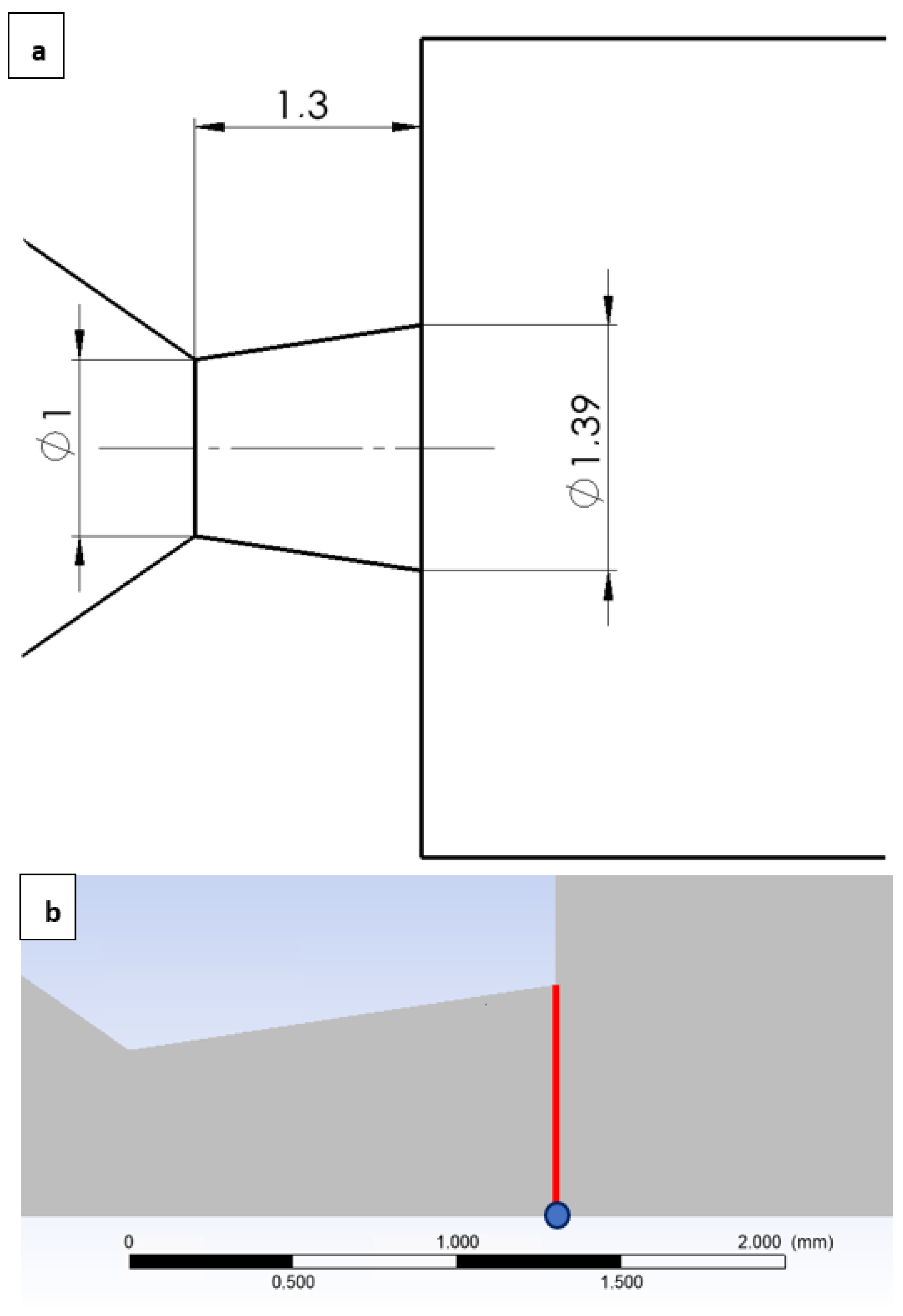
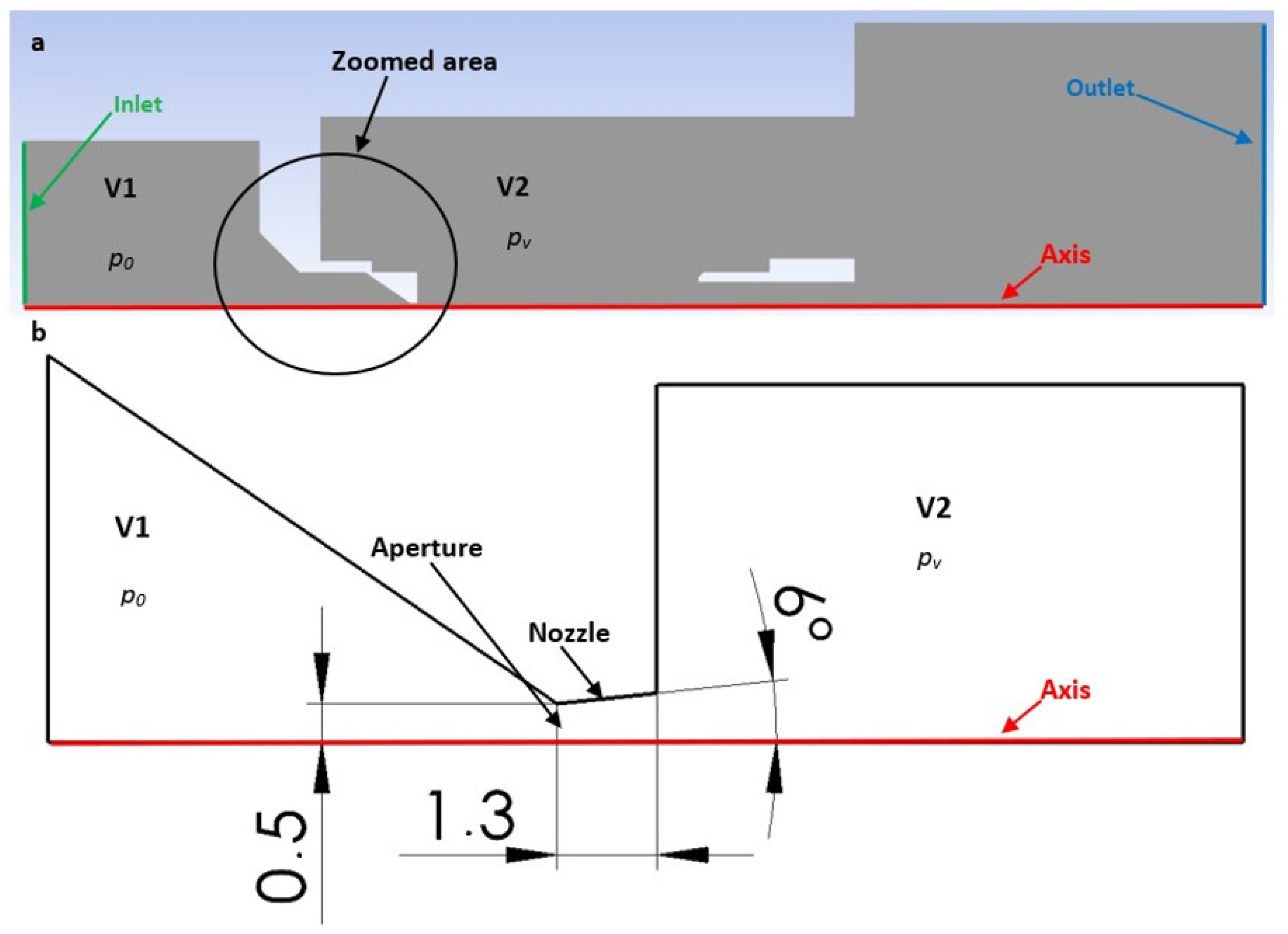
| Aperture | 0.0022 | 1.56 | 0.73 | 297.7 | 2 | 254.5 |
| Nozzle | 0.005 | 0.803 | 0.075 | 602.1 | 3.88 | 120.4 |
| Point on Path [mm] | Char. Dimension [m] | Mean Velocity [m·s−1] | Density [kg·m−3] | Dyn. Viscosity [Pa·s] | Temperature [K] | Re Number [-] |
|---|---|---|---|---|---|---|
| 0 | 0.002 | 148.85 | 0.73 | 1.56 × 10⁻⁵ | 254.5 | 13,930.83 |
| 2.5 | 0.0027 | 142.55 | 0.241 | 1.57 × 10⁻⁵ | 255.5 | 5908.11 |
| 5 | 0.0035 | 287.4 | 0.095 | 8.98 × 10⁻⁵ | 135.2 | 10,641.48 |
| 7.5 | 0.08 | 118.3 | 0.196 | 1.63 × 10⁻⁵ | 268.5 | 111,730.47 |
| Variant (Further Marked) | p0 (Input Pressure) [Pa] | pv (Output Pressure) [Pa] |
|---|---|---|
| 101,325 Pa | 1,013,250 | 101,325 |
| 50,000 Pa | 500,000 | 50,000 |
| 10,000 Pa | 100,000 | 10,000 |
| 5000 Pa | 50,000 | 5000 |
| 2000 Pa | 20,000 | 2000 |
| Labeling | Unit | Theory | |
|---|---|---|---|
| Mach number | Mv | [-] | 2.16 |
| Speed of sound in the chamber for T0 = 24 °C | a0 | [m·s−1] | 345.5 |
| Outlet speed of sound | av | [m·s−1] | 248.5 |
| Outlet velocity | vv | [m·s−1] | 536.8 |
| Outlet temperature | Tv | [K] | 153.7 |
| Outlet cross-section | Av | [mm2] | 1.39 |
| Labeling | Unit | Theory | Point | Line | |
|---|---|---|---|---|---|
| Mach number | Mv | [-] | 2.16 | 2 | 2.1 |
| Speed of sound in the chamber for T0 = 24 °C | a0 | [m·s−1] | 345.5 | - | - |
| Outlet speed of sound | av | [m·s−1] | 248.5 | - | - |
| Outlet velocity | vv | [m·s−1] | 536.8 | 530.9 | 530 |
| Outlet temperature | Tv | [K] | 153.7 | 160 | 157 |
| Outlet cross-section | Av | [mm2] | 1.39 | - | - |
| Variant 101,325 Pa | |||||
| Outlet static pressure | pv | [Pa] | 101,325 | 250,906 | 102,324 |
| Outlet density | ρv | [kg·m−3] | 2.29 | 2.9 | 2.2 |
| Variant 50,000 Pa | |||||
| Outlet static pressure | pv | [Pa] | 50,000 | 130,398 | 50,906 |
| Outlet density | ρv | [kg·m−3] | 1.13 | 1.48 | 1.1 |
| Variant 10,000 Pa | |||||
| Outlet static pressure | pv | [Pa] | 10,000 | 13,924 | 10,569 |
| Outlet density | ρv | [kg·m−3] | 0.226 | 0.29 | 0.227 |
| Variant 5000 Pa | |||||
| Outlet static pressure | pv | [Pa] | 5000 | 6580 | 5495 |
| Outlet density | ρv | [kg·m−3] | 0.113 | 0.126 | 0.116 |
| Variant 2000 Pa | |||||
| Outlet static pressure | pv | [Pa] | 2000 | 2506 | 2288 |
| Outlet density | ρv | [kg·m−3] | 0.045 | 0.051 | 0.049 |
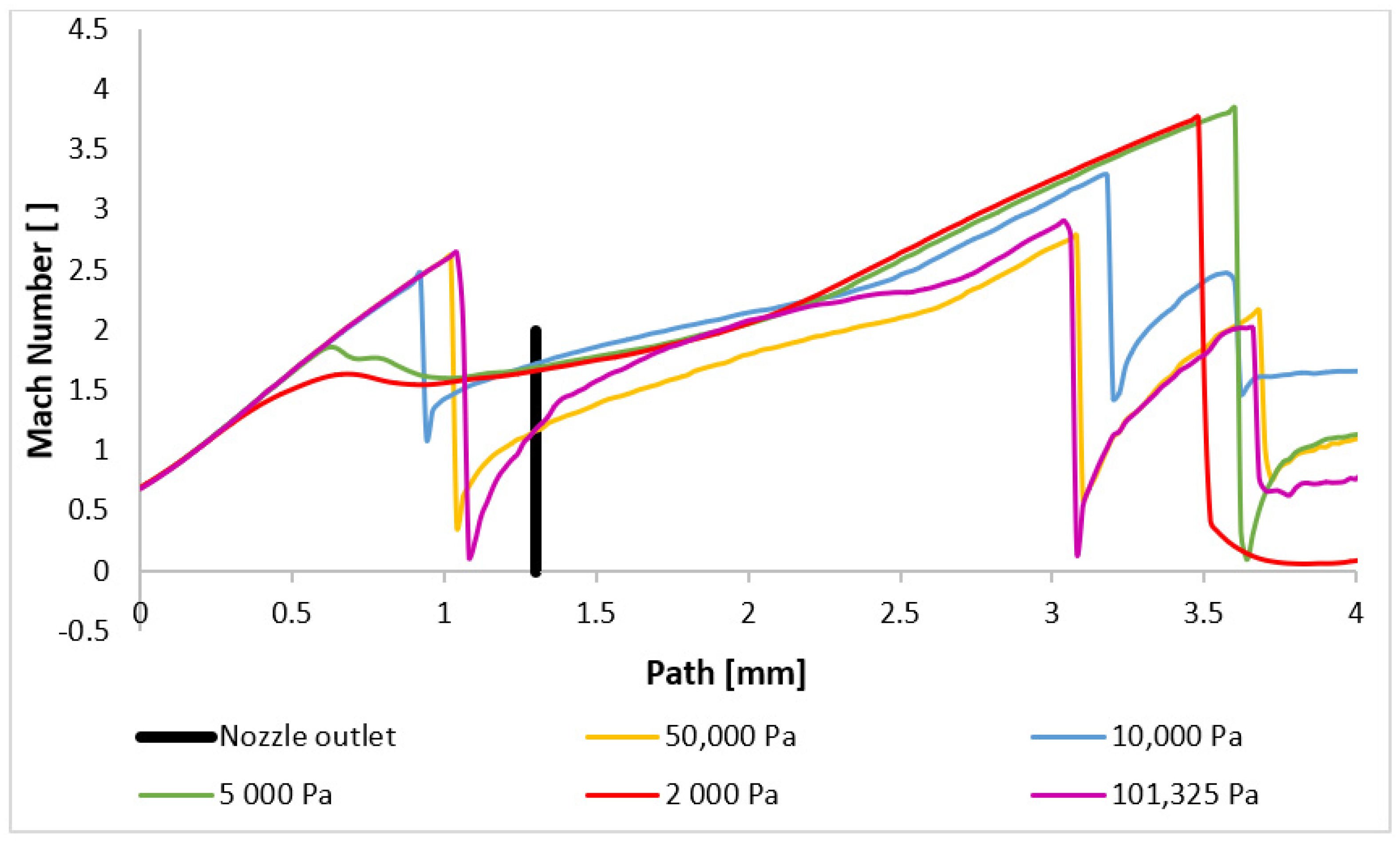
| Shock Wave Position | |||
|---|---|---|---|
| Variant | 1 [mm] | 2 [mm] | 3 [mm] |
| 101,325 Pa | 1.06 | 3.06 | 3.68 |
| 50,000 Pa | 1.04 | 3.1 | 3.7 |
| 10,000 Pa | 0.92 | 3.2 | 3.62 |
| 5000 Pa | - | - | 3.62 |
| 2000 Pa | - | - | 3.5 |
| Variant | Point | Char. Dimension [m] | Mean Velocity [m·s−1] | Density [kg·m−3] | Dyn. Viscosity [Pa·s] | Temperature [K] | Re Number [-] |
|---|---|---|---|---|---|---|---|
| 101,325 Pa | 1 | 0.00113 | 258.5 | 2.74 | 1.09 × 10⁻⁵ | 167 | 73,428.23 |
| 2 | 0.00127 | 186 | 2.91 | 1.43 × 10⁻⁵ | 229 | 41,935.86 | |
| 3 | 0.08 | 246 | 1.73 | 1.16 × 10⁻⁵ | 178 | 2,935,034.48 | |
| 50,000 Pa | 1 | 0.00113 | 259 | 1.35 | 1.09 × 10⁻⁵ | 167 | 36,248.12 |
| 2 | 0.00127 | 182.5 | 1.36 | 1.45 × 10⁻⁵ | 232 | 21,738.9 | |
| 3 | 0.08 | 241 | 0.84 | 1.18 × 10⁻⁵ | 181.6 | 1,372,474.58 | |
| 10,000 Pa | 1 | 0.00113 | 259 | 0.27 | 1.1 × 10⁻⁵ | 168 | 7203.36 |
| 2 | 0.00127 | 239.5 | 0.323 | 1.2 × 10⁻⁵ | 186 | 8180.29 | |
| 3 | 0.08 | 272.5 | 0.208 | 1.01 × 10⁻⁵ | 154 | 448,950.5 | |
| 5000 Pa | 1 | 0.00113 | 258.5 | 0.137 | 1.1 × 10⁻⁵ | 169 | 3624.85 |
| 2 | 0.00127 | 245 | 0.165 | 1.18 × 10⁻⁵ | 182 | 4350.83 | |
| 3 | 0.08 | 273 | 0.109 | 1.01 × 10⁻⁵ | 154 | 234,769.23 | |
| 2000 Pa | 1 | 0.00113 | 242 | 0.0685 | 1.196 × 10⁻⁵ | 184 | 1574.12 |
| 2 | 0.00127 | 243.5 | 0.067 | 1.18 × 10⁻⁵ | 183 | 1755.88 | |
| 3 | 0.08 | 269.5 | 0.046 | 1.03 × 10⁻⁵ | 157 | 96,287.38 |
Disclaimer/Publisher’s Note: The statements, opinions and data contained in all publications are solely those of the individual author(s) and contributor(s) and not of MDPI and/or the editor(s). MDPI and/or the editor(s) disclaim responsibility for any injury to people or property resulting from any ideas, methods, instructions or products referred to in the content. |
© 2024 by the authors. Licensee MDPI, Basel, Switzerland. This article is an open access article distributed under the terms and conditions of the Creative Commons Attribution (CC BY) license (https://creativecommons.org/licenses/by/4.0/).
Share and Cite
Bayer, R.; Bača, P.; Maxa, J.; Šabacká, P.; Binar, T.; Vyroubal, P. CFD Analyses of Density Gradients under Conditions of Supersonic Flow at Low Pressures. Sensors 2024, 24, 5968. https://doi.org/10.3390/s24185968
Bayer R, Bača P, Maxa J, Šabacká P, Binar T, Vyroubal P. CFD Analyses of Density Gradients under Conditions of Supersonic Flow at Low Pressures. Sensors. 2024; 24(18):5968. https://doi.org/10.3390/s24185968
Chicago/Turabian StyleBayer, Robert, Petr Bača, Jiří Maxa, Pavla Šabacká, Tomáš Binar, and Petr Vyroubal. 2024. "CFD Analyses of Density Gradients under Conditions of Supersonic Flow at Low Pressures" Sensors 24, no. 18: 5968. https://doi.org/10.3390/s24185968