
Research on Signal Noise Reduction and Leakage Localization in Urban Water Supply Pipelines Based on Northern Goshawk Optimization

Abstract
1. Introduction
2. Methodology
2.1. Principle of VMD
2.2. Northern Goshawk Optimization
2.2.1. Principle of NGO
- Phase 1: Prey identification (exploration phase)
- Phase 2: Chase and escape (development phase)
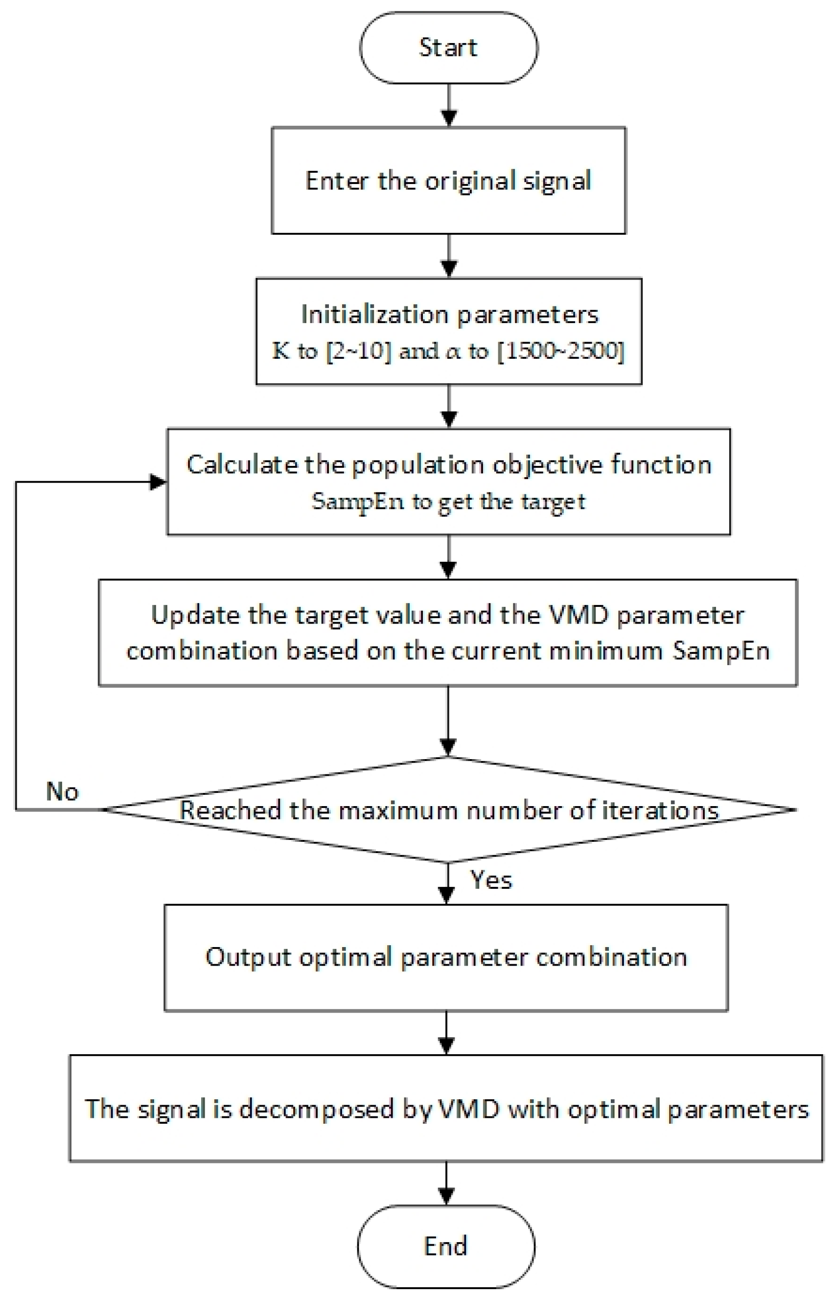
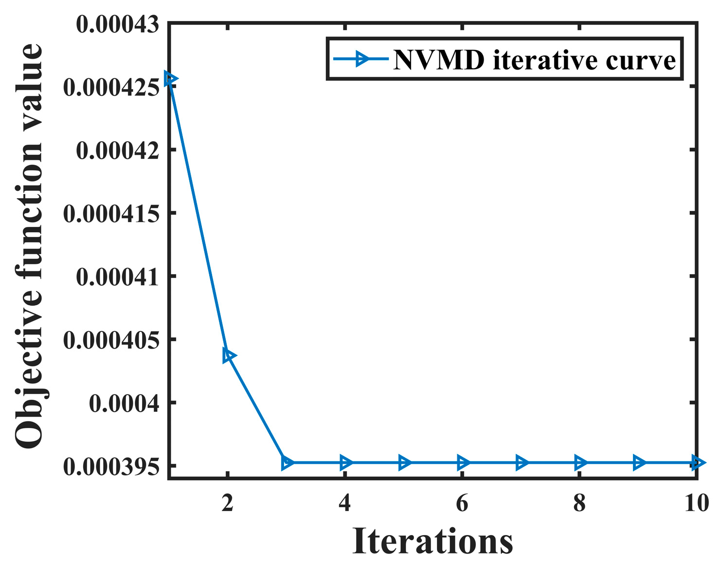
2.2.2. VMD Based on NGO
2.2.3. Evaluation Indicators
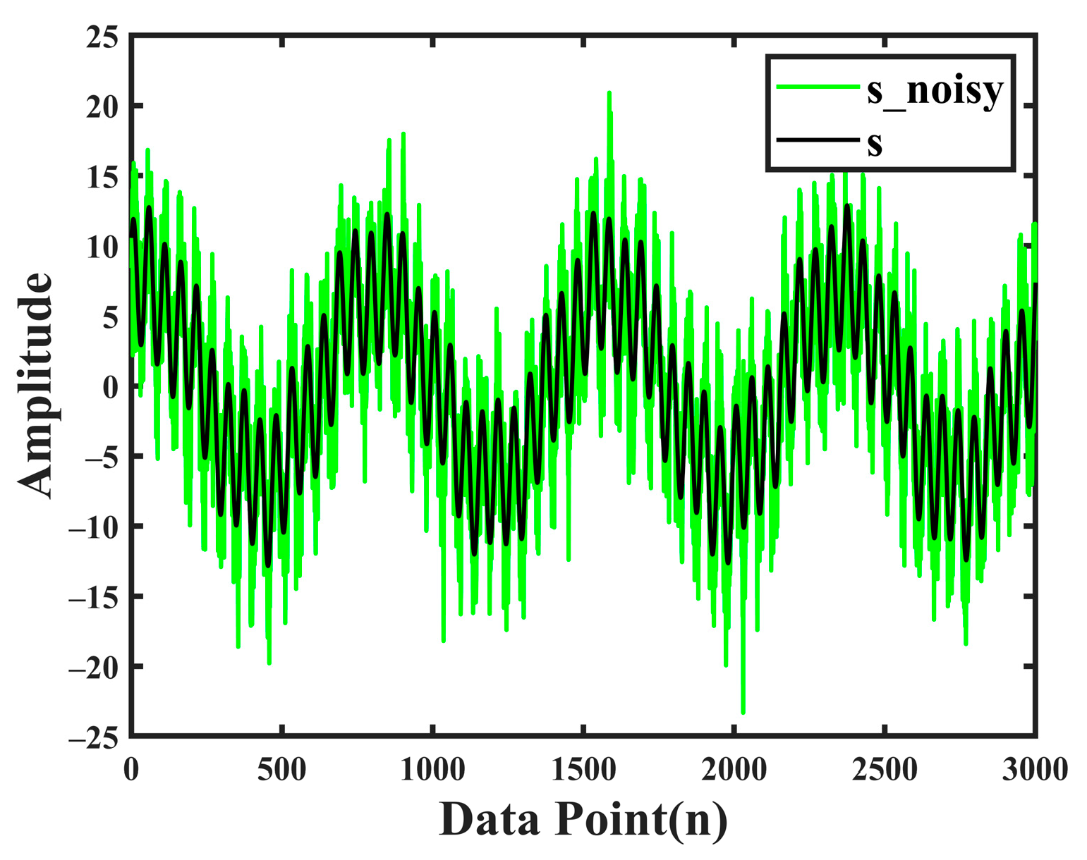
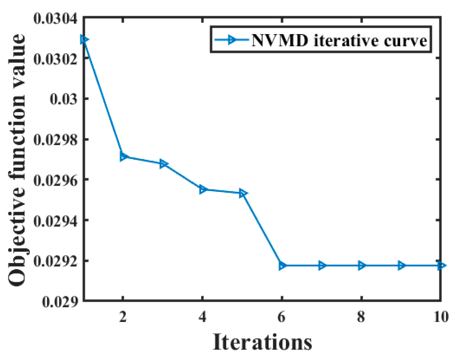
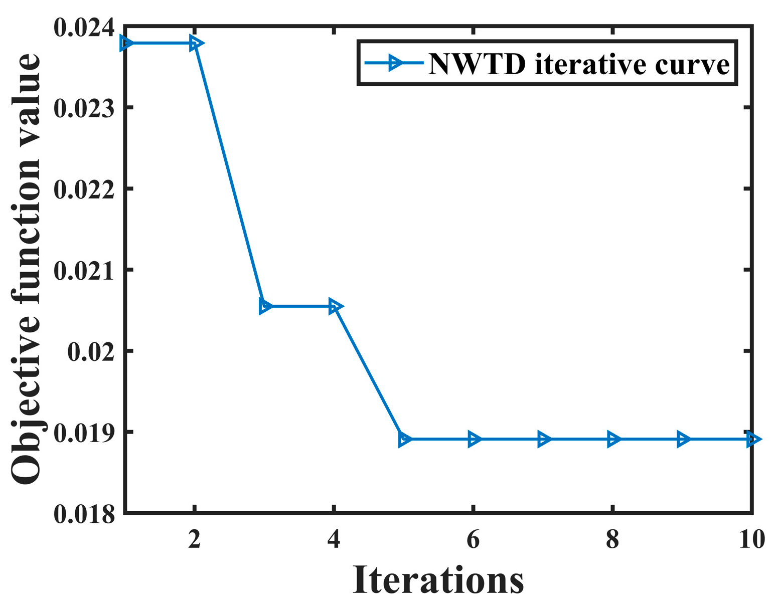
2.3. Simulation Test Verification
3. Leak Location Based on Improved VMD
3.1. Pipe Leakage Location Principle Based on NPW
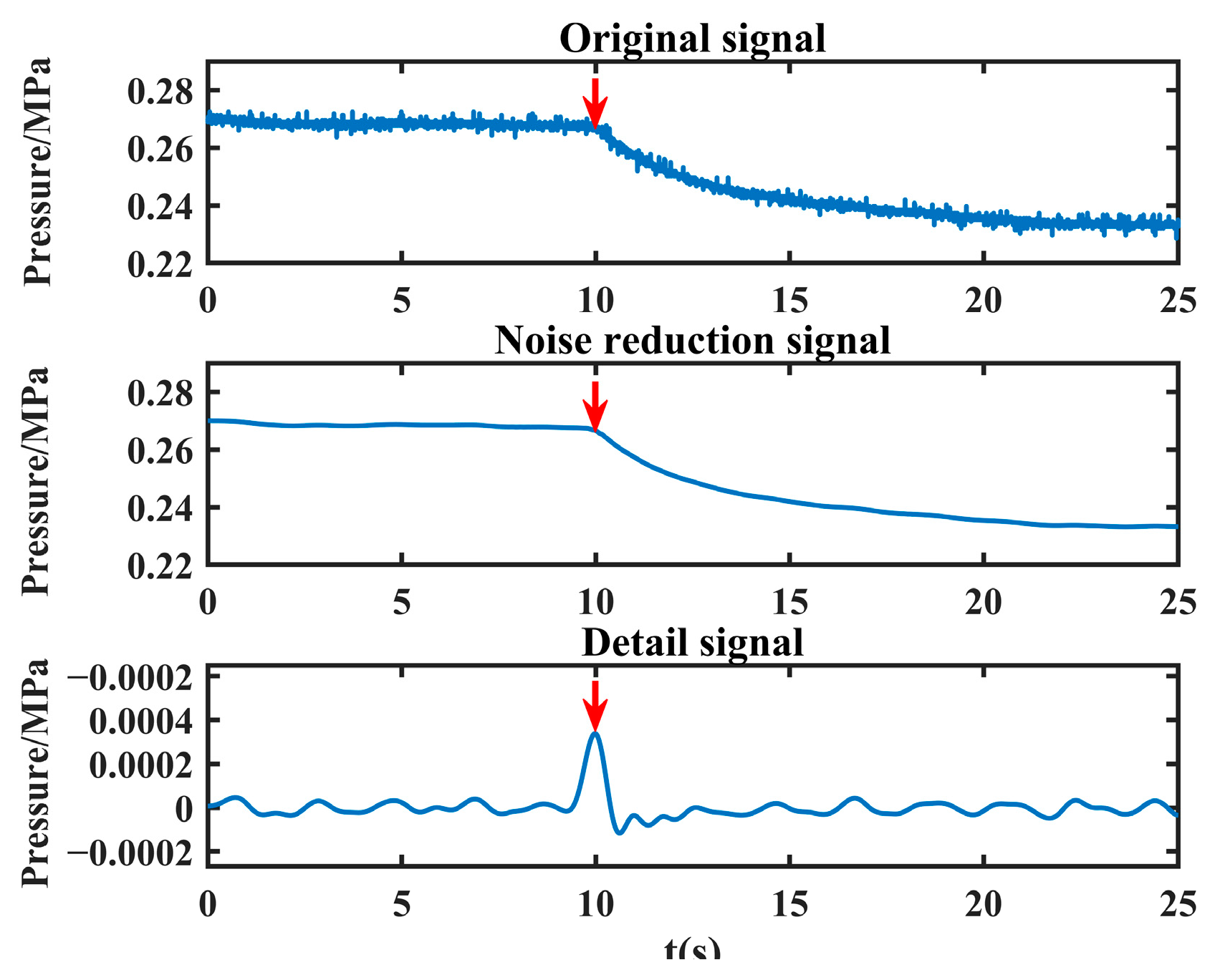
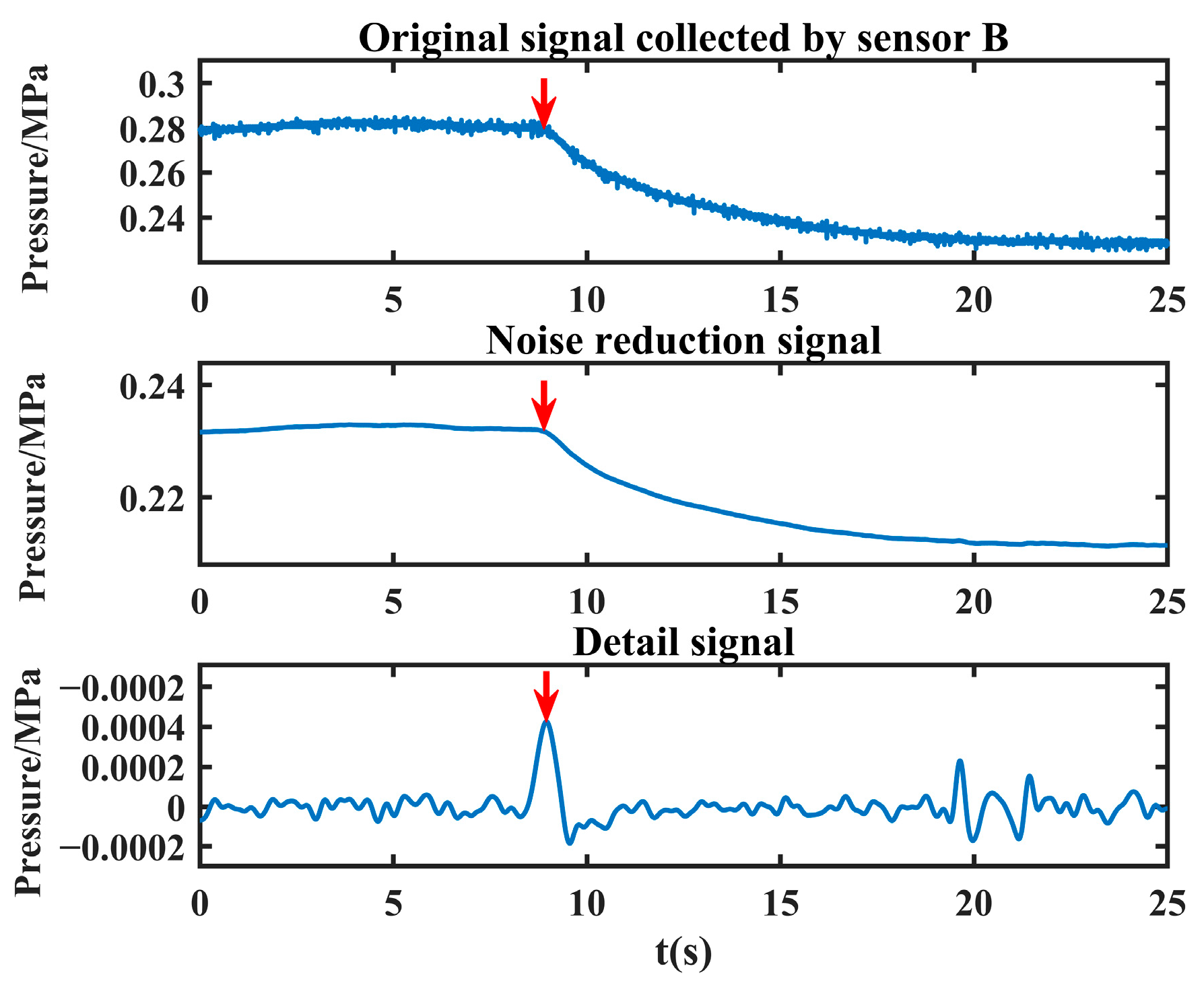
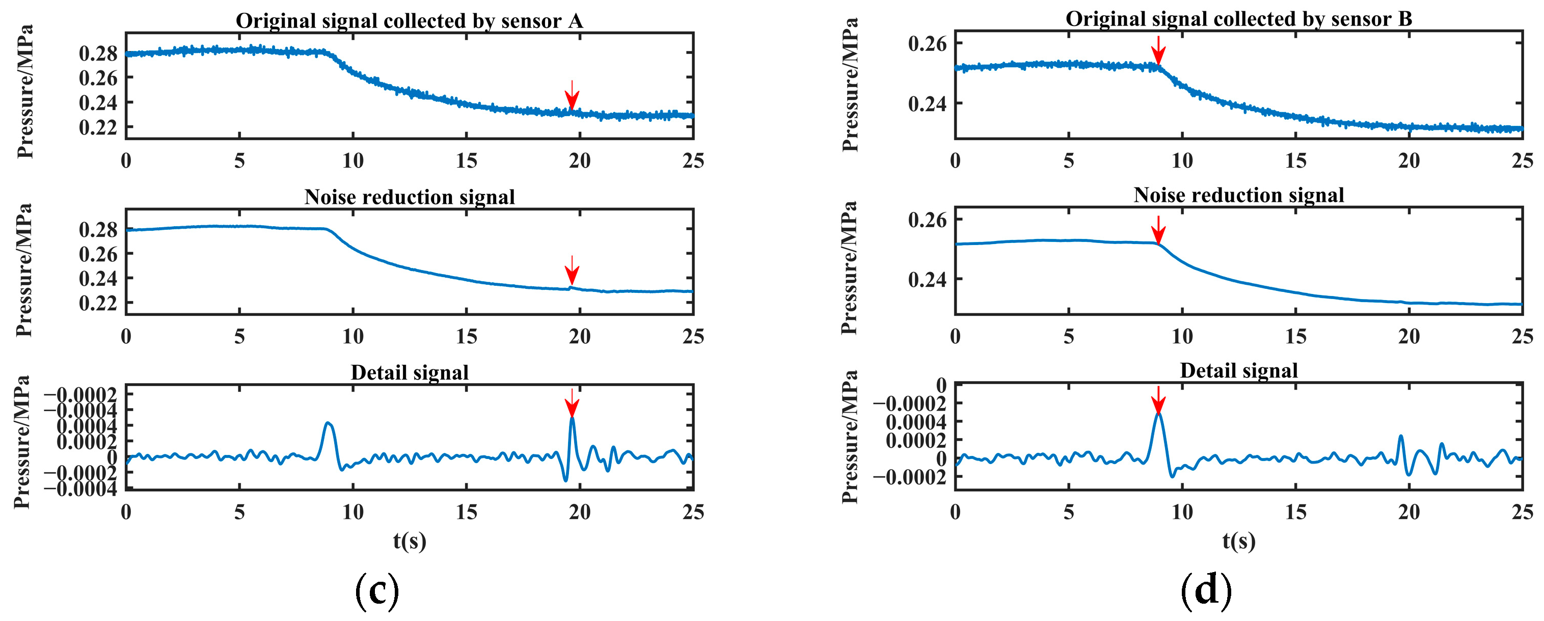
3.2. Leakage Singularity Extraction
4. Test Analyses
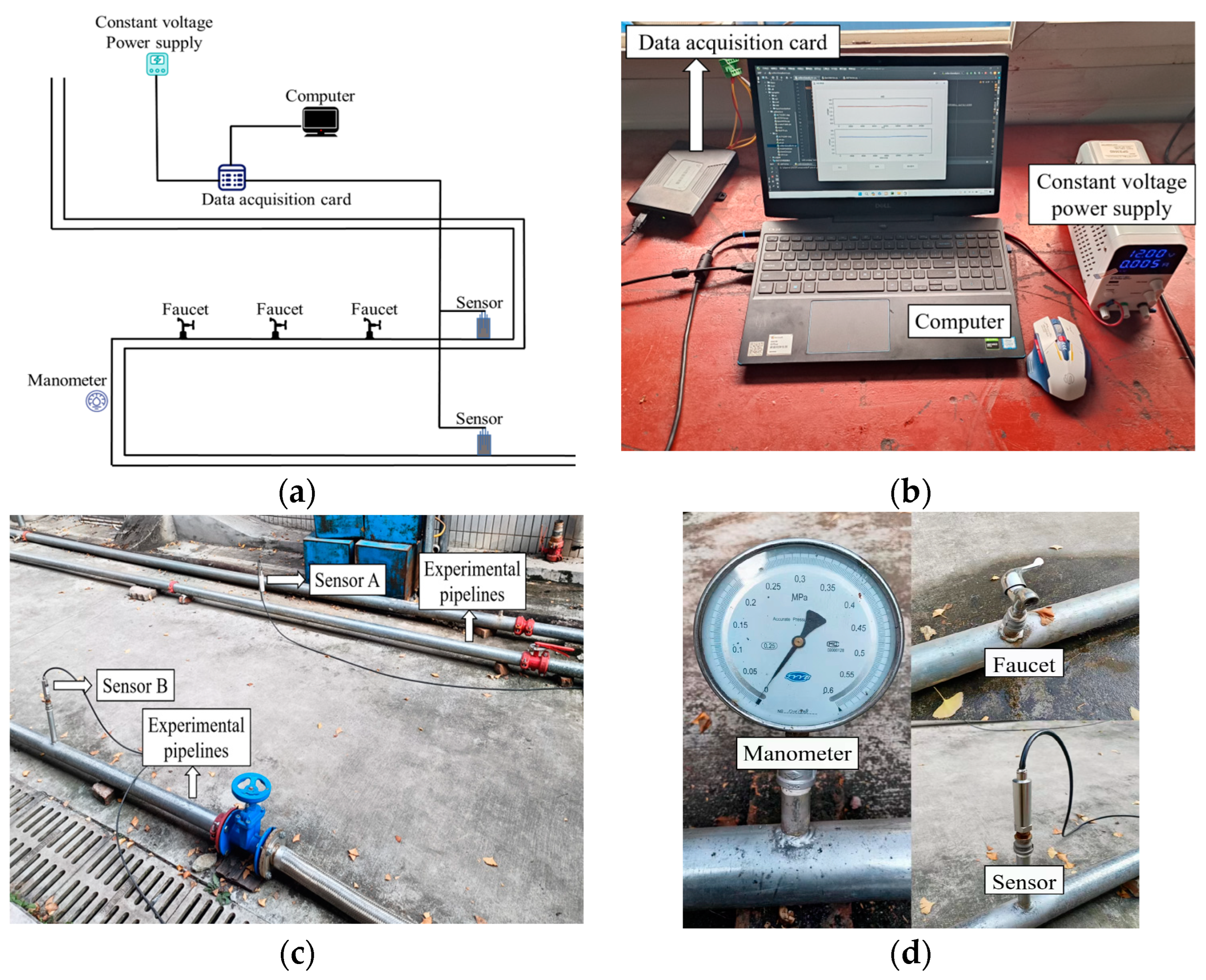
4.1. Test Equipment
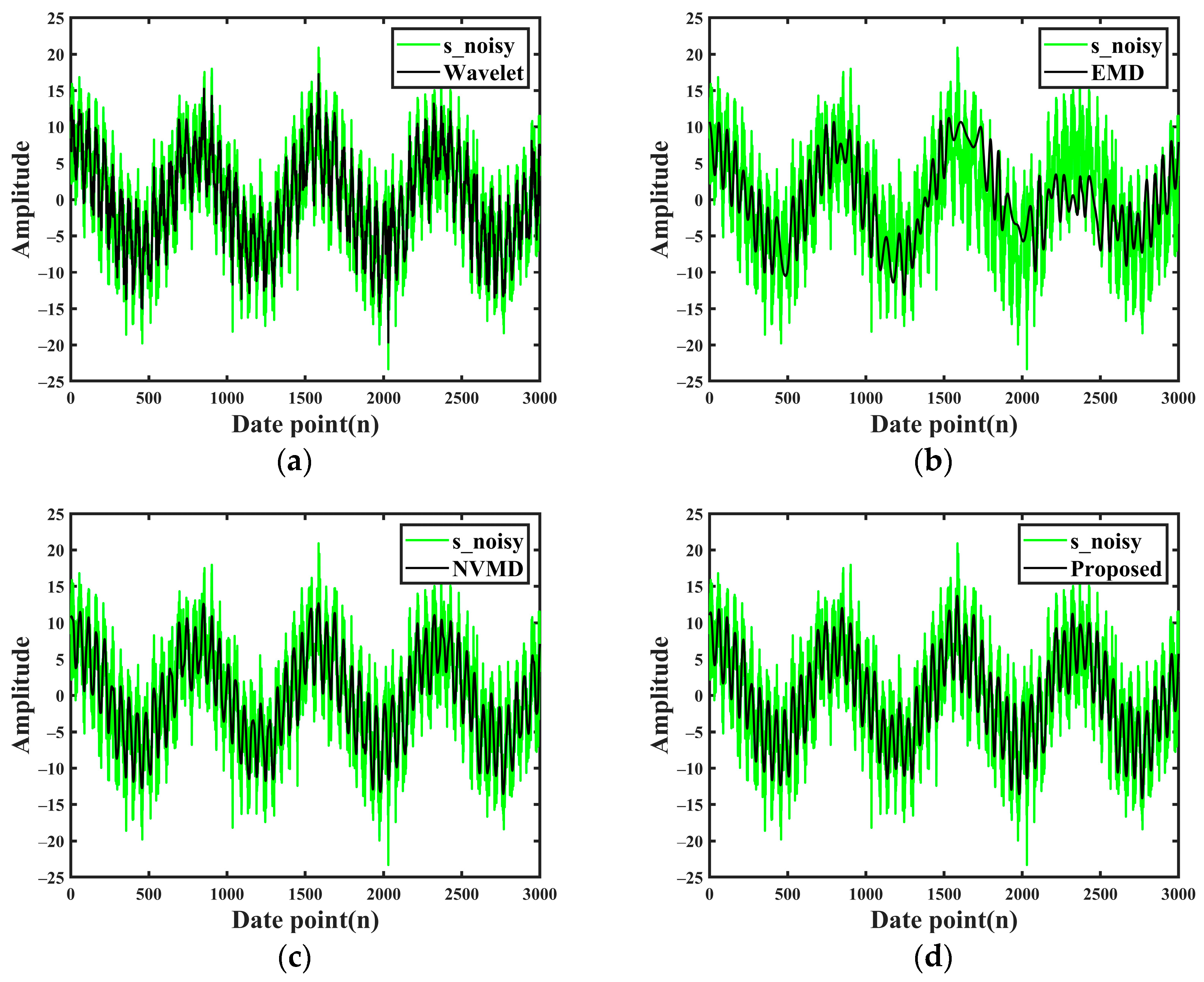
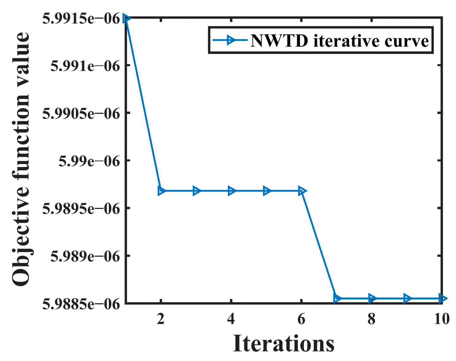
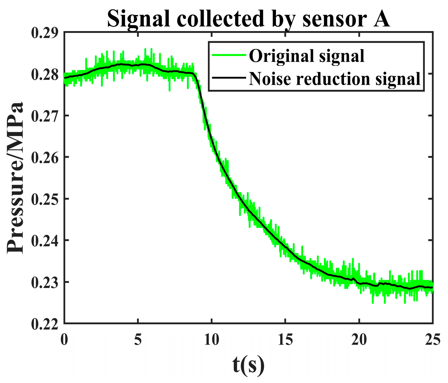
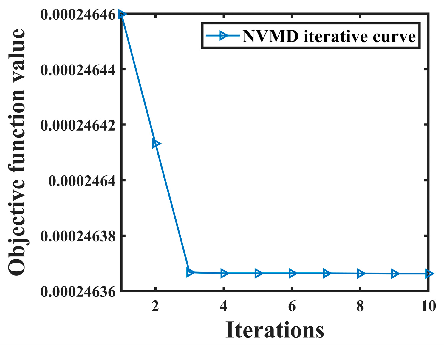
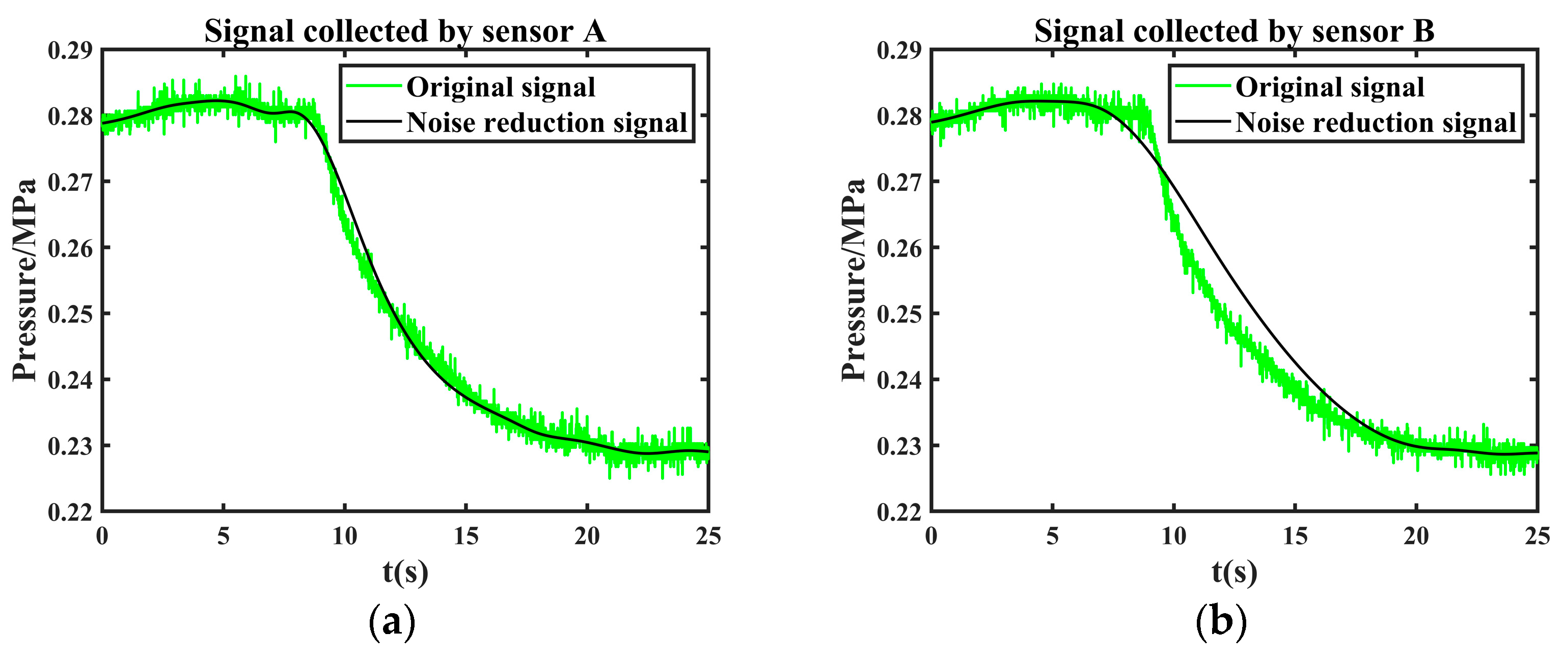
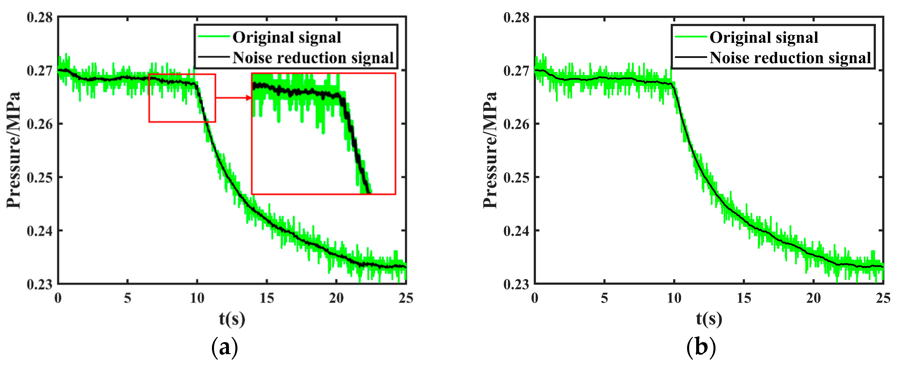
4.2. Joint Noise Reduction for Leakage Signals
4.3. Leak Location
4.4. Comparison of Methods
5. Conclusions
Author Contributions
Funding
Institutional Review Board Statement
Informed Consent Statement
Data Availability Statement
Conflicts of Interest
References
- Ye, B.; Ma, Y.; Zhang, L.; Yu, F. Research on ecological environment construction and water resources protection and utilization. Environ. Sci. Manag. 2022, 47, 22–25+48. [Google Scholar]
- Zhang, Z. Research on Time-Domain Convolution and Positional Regression Based Leakage Time Localisation Method for Water Pipe Network. Master’s Thesis, Xi’an University of Technology, Xi’an, China, 2023. [Google Scholar]
- Li, S.; Xia, C.; Cheng, Z.; Mao, W.; Liu, Y.; Habibi, D. Leak location based on PDS-VMD of leakage-induced vibration signal under low SNR in water-supply pipelines. IEEE Access 2020, 8, 68091–68102. [Google Scholar] [CrossRef]
- Hasan, F.; Iqbal, J. Consequential rupture of gas pipeline. Eng. Fail. Anal. 2004, 13, 127–135. [Google Scholar] [CrossRef]
- Pallavi, V.; Mukherjee, J.; Majumdar, A.K.; Sural, S. Ball detection from broadcast soccer videos using static and dynamic features. J. Vis. Commun. Image Represent. 2008, 19, 426–436. [Google Scholar] [CrossRef]
- Ancona, N.; Cicirelli, G.; Stella, E.; Distante, A. Ball detection in static images with Support Vector Machines for classification. Image Vis. Comput. 2003, 21, 675–692. [Google Scholar] [CrossRef]
- Montiel, H.; Vílchez, J.A.; Casal, J.; Arnaldos, J. Mathematical modeling of accidental gas release. J. Hazard. Mater. 1998, 59, 211–233. [Google Scholar] [CrossRef]
- Hiroki, S.; Tanzawa, S.; Arai, T. Development of Water Leak Detection Method in Fusion Reactors Using Water-Soluble Gas Fusion. Eng. Des. 2008, 83, 72–78. [Google Scholar] [CrossRef]
- Reich, G. Leak Detection with Tracer Gases. Sensit. Relev. Limiting Factors Vac. 2006, 37, 691–698. [Google Scholar]
- Sun, A.; Chen, J.; Li, G.; Wang, L.; Chang, L.; Lin, Z. Detection of Spontaneou Brillou in Back Scattered Powering Distributed Optical Fiber Sensor System Based on High Frequency Microwave Technology. China. J. Lasers 2007, 34, 503–506. [Google Scholar]
- Li, R. Research and Application of Negative Pressure Wave Pipeline Leakage Detection Based on Combined Signal Processing. Master’s Thesis, Xi’an Petroleum University, Xian, China, 2023. [Google Scholar]
- Stouffs, P.; Giot, M. Pipeline Leak Detection Based on Mass Balance: Importance of The Packing Term. J. Loss Prev. Process Ind. 1993, 6, 307–312. [Google Scholar] [CrossRef]
- Ge, C.; Wang, G.; Ye, H. Analysis of the Smallest Detectable Leakage Flow Rate of Negative Pressure Wave Based Leak Detection Symtemsfor Liquid Pipelines. Comput. Chem. Eng. 2008, 32, 42–46. [Google Scholar] [CrossRef]
- Kam, S.I. Mechanistic Modeling of Pipeline Leak Detection at Fixed Inlet Rate. J. Pet. Sci. Eng. 2010, 70, 145–156. [Google Scholar] [CrossRef]
- Doshmanziari, R.; Khaloozadeh, H.; Nikoofard, A. Gas pipeline leakage detection based on sensor fusion under model-based fault detection framework. J. Petorleum Sci. Eng. 2020, 188, 106581. [Google Scholar] [CrossRef]
- Wei, Y. Research on Pipeline Signal Recognition Method Based on CEEMDAN and ELM. Master’s Thesis, Northeast Petroleum University, Daqing, China, 2023. [Google Scholar]
- Liu, B. Research on Water Supply Pipe Leakage Detection and Localisation Method Based on Variational Modal Decomposition; Xihua University: Chengdu, China, 2022. [Google Scholar] [CrossRef]
- Wang, P. Application of Empirical Modal Decomposition in Noise Reduction and Feature Extraction of Hydroacoustic Signals. Master’s Thesis, Guilin University of Electronic Science and Technology, Guilin, China, 2023. [Google Scholar]
- Zhang, L.; Bao, P.; Wu, X. Multiscale LMMSE-based image denoising with optimal wavelet selection. IEEE Trans. Circuits Syst. Video Technol. 2005, 15, 469–481. [Google Scholar] [CrossRef]
- Huang, N.E.; Shen, Z.; Long, S.R.; Wu, M.C.; Shih, H.H.; Zheng, Q.; Yen, N.C.; Tung, C.C.; Liu, H.H. The empirical mode decomposition and the Hilbert spectrum for nonlinear and non-stationary time series analysis. Proc. R. Soc. Lond. Ser. A Math. Phys. Eng. Sci. 1998, 454, 903–995. [Google Scholar] [CrossRef]
- Nguyen, P.; Kang, M.; Kim, J.M.; Ahn, B.H.; Ha, J.M.; Choi, B.K. Robust condition monitoring of rolling element bearings using de-noising and envelope analysis with signal decomposition techniques. Expert Syst. Appl. 2015, 42, 9024–9032. [Google Scholar] [CrossRef]
- Bharathi, B.M.R.; Mohanty, A.R. Time delay estimation in reverberant and low SNR environment by EMD based maximum likelihood method. Measurement 2019, 137, 655–663. [Google Scholar] [CrossRef]
- Shang, X.-Q.; Huang, T.-L.; Chen, H.-P.; Ren, W.-X.; Lou, M.-L. Recursive variational mode decomposition enhanced by orthogonalization algorithm for accurate structural modal identification. Mech. Syst. Sig. Process. 2023, 197, 110–358. [Google Scholar] [CrossRef]
- Dehghani, M.; Hubálovský, Š.; Trojovský, P. Northern Goshawk Optimization: A New Swarm-Based Algorithm for Solving Optimization Problems. IEEE Access 2021, 9, 162059–162080. [Google Scholar] [CrossRef]
- Dragomiretskiy, K.; Zosso, D. Variational mode decomposition. IEEE Trans. Signal Process. 2014, 62, 531–544. [Google Scholar] [CrossRef]
- Richman, J.S.; Moorman, J.R. Physiological time-series analysis using approximate entropy and sample entropy. Am. J. Physiol. Heart Circ. Physiol. 2000, 278, H2039–H2049. [Google Scholar] [CrossRef] [PubMed]
- Xu, Y.; Cheng, S.; Xue, Y. DC distribution network protection based on Pearson correlation coefficient of fault transient current. J. North China Electr. Power Univ. (Nat. Sci. Ed.) 2021, 48, 11–19. [Google Scholar]
- Shen, C.; Wu, X.; Zhao, D.; Li, S.; Cao, H.; Zhao, H.; Tang, J.; Liu, J.; Wang, C. Comprehensive heading error processing technique using image denoising and tilt-induced error compensation for polarization compass. IEEE Access 2020, 8, 187222–187231. [Google Scholar] [CrossRef]
- Lei, W.; Wang, G.; Wan, B.; Min, Y.; Wu, J.; Li, B. High voltage shunt reactor acoustic signal denoising based on the combination of VMD parameters optimized by coati optimization algorithm and wavelet threshold. Measurement 2024, 224, 113854. [Google Scholar] [CrossRef]
- Ayat, M.; Shamsollahi, M.B.; Mozaffari, B.; Kharabian, S. ECG de-noising using modulus maxima of wavelet transform. In Proceedings of the 2009 Annual International Conference of the IEEE Engineering in Medicine and Biology Society, Minneapolis, MN, USA, 3–6 September 2009; pp. 416–419. [Google Scholar]
- Singh, P.; Pradhan, G.; Shahnawazuddin, S. Denoising of ECG signal by non-local estimation of approximation coefficients in DWT. Biocybern. Biomed. Eng. 2017, 37, 599–610. [Google Scholar] [CrossRef]
- Shi, H.; Liu, R.; Chen, C.; Shu, M.; Wang, Y. ECG baseline estimation and denoising with group sparse regularization. IEEE Access 2021, 9, 23595–23607. [Google Scholar] [CrossRef]
- Wang, J.; Ren, L.; Jiang, T.; Jia, Z.; Wang, G.X. A novel gas pipeline burst detection and localization method based on the FBG caliber-based sensor array. Measurement 2020, 151, 107226. [Google Scholar] [CrossRef]
- Wang, J. Research on Intelligent Leakage Detection and Positioning of Multi-Condition Pipelines Based on Signal Processing. Master’s Thesis, Xi’an Petroleum University, Xi’an, China, 2023. [Google Scholar]


| IMF | cc | IMF | cc |
|---|---|---|---|
| IMF1 | 1.2382 × 10⁻⁵ | IMF6 | 5.9675 × 10⁻⁵ |
| IMF2 | 1.3246 × 10⁻⁵ | IMF7 | 8.2930 × 10⁻⁵ |
| IMF3 | 2.0955 × 10⁻⁵ | IMF8 | 5.3093 × 10⁻⁴ |
| IMF4 | 1.0313 × 10⁻⁵ | IMF9 | 0.5670 |
| IMF5 | 2.4869 × 10⁻⁵ | IMF10 | 0.8146 |
| Noise Reduction Methods | SNR/dB | NCC |
|---|---|---|
| Wavelet | 11.85 | 0.968 |
| EMD | 4.51 | 0.810 |
| NVMD | 16.09 | 0.988 |
| Our method | 17.23 | 0.991 |
| IMF | cc | IMF | cc |
|---|---|---|---|
| IMF1 | −4.25 × 10⁻⁴ | IMF6 | 9.40 × 10⁻⁴ |
| IMF2 | −5.53 × 10⁻⁵ | IMF7 | 1.72 × 10⁻⁴ |
| IMF3 | 4.72 × 10⁻⁴ | IMF8 | 8.61 × 10⁻⁴ |
| IMF4 | 8.11 × 10⁻⁵ | IMF9 | 0.0027 |
| IMF5 | 2.50 × 10⁻⁴ | IMF10 | 0.9996 |
| (m) | Leak | (m) | t1 (s) | t2 (s) | (s) | (m) | (m) | (%) | |
|---|---|---|---|---|---|---|---|---|---|
| 27.86 | 1 | 1 | 4.01 | 7.168 | 7.188 | −0.020 | 3.93 | 0.08 | 0.29 |
| 2 | 9.230 | 9.248 | −0.018 | 4.93 | 0.92 | 3.30 | |||
| 3 | 11.480 | 11.500 | −0.020 | 3.93 | 0.08 | 0.29 | |||
| 2 | 4 | 7.1 | 4.684 | 4.696 | −0.012 | 7.93 | 0.83 | 2.98 | |
| 5 | 8.402 | 8.414 | −0.012 | 7.93 | 0.83 | 2.98 | |||
| 6 | 9.982 | 9.996 | −0.014 | 6.93 | 0.17 | 0.61 | |||
| 3 | 7 | 10.12 | 3.060 | 3.068 | −0.008 | 9.93 | 0.19 | 0.68 | |
| 8 | 3.602 | 3.610 | −0.008 | 9.93 | 0.19 | 0.68 | |||
| 9 | 8.946 | 8.952 | −0.006 | 10.93 | 0.81 | 2.91 |
| (m) | Leak | (m) | Z1 (m) | 1 (%) | Z2 (m) | 2 (%) | Z3 (m) | 3 (%) | |
|---|---|---|---|---|---|---|---|---|---|
| 27.86 | 1 | 1 | 4.01 | — | — | 1.93 | 7.47 | — | — |
| 2 | — | — | 6.93 | 10.48 | — | — | |||
| 3 | — | — | 5.93 | 6.89 | — | — | |||
| 2 | 4 | 7.1 | — | — | — | — | — | — | |
| 5 | — | — | — | — | — | — | |||
| 6 | — | — | 5.93 | 4.20 | — | — | |||
| 3 | 7 | 10.12 | — | — | 8.93 | 4.27 | — | — | |
| 8 | — | — | — | — | — | — | |||
| 9 | — | — | — | — | — | — |
Disclaimer/Publisher’s Note: The statements, opinions and data contained in all publications are solely those of the individual author(s) and contributor(s) and not of MDPI and/or the editor(s). MDPI and/or the editor(s) disclaim responsibility for any injury to people or property resulting from any ideas, methods, instructions or products referred to in the content. |
© 2024 by the authors. Licensee MDPI, Basel, Switzerland. This article is an open access article distributed under the terms and conditions of the Creative Commons Attribution (CC BY) license (https://creativecommons.org/licenses/by/4.0/).
Share and Cite
Chen, X.; Jiang, Z.; Li, J.; Zhao, Z.; Cao, Y. Research on Signal Noise Reduction and Leakage Localization in Urban Water Supply Pipelines Based on Northern Goshawk Optimization. Sensors 2024, 24, 6091. https://doi.org/10.3390/s24186091
Chen X, Jiang Z, Li J, Zhao Z, Cao Y. Research on Signal Noise Reduction and Leakage Localization in Urban Water Supply Pipelines Based on Northern Goshawk Optimization. Sensors. 2024; 24(18):6091. https://doi.org/10.3390/s24186091
Chicago/Turabian StyleChen, Xin, Zhu Jiang, Jiale Li, Zhendong Zhao, and Yunyun Cao. 2024. "Research on Signal Noise Reduction and Leakage Localization in Urban Water Supply Pipelines Based on Northern Goshawk Optimization" Sensors 24, no. 18: 6091. https://doi.org/10.3390/s24186091
APA StyleChen, X., Jiang, Z., Li, J., Zhao, Z., & Cao, Y. (2024). Research on Signal Noise Reduction and Leakage Localization in Urban Water Supply Pipelines Based on Northern Goshawk Optimization. Sensors, 24(18), 6091. https://doi.org/10.3390/s24186091