
Investigation of the Robust Integration of Distributed Fibre Optic Sensors in Structural Concrete Components


Abstract
1. Introduction
2. Literature Study
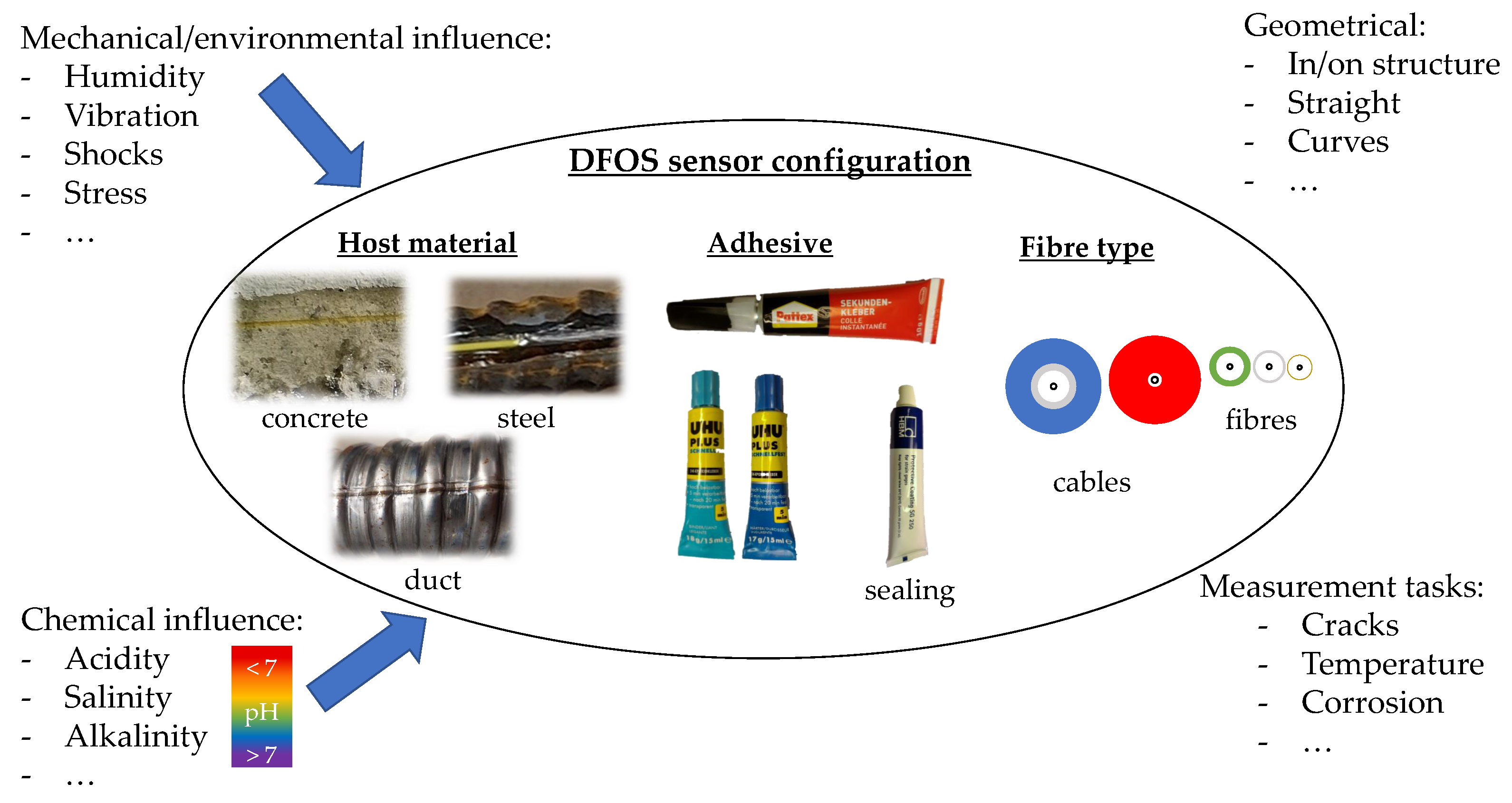
2.1. Sensor Configuration
2.2. Fibre Type
2.3. Adhesives and Host Materials
2.4. Conclusions of DFOS Sensor Configuration
2.5. Validation
3. Embedding Fibres into Concrete Structures
4. Use of Ducts as Host Material
4.1. Tendons and Their Role in Prestressed Concrete
4.2. Basic Idea and Specimens
4.3. Theory
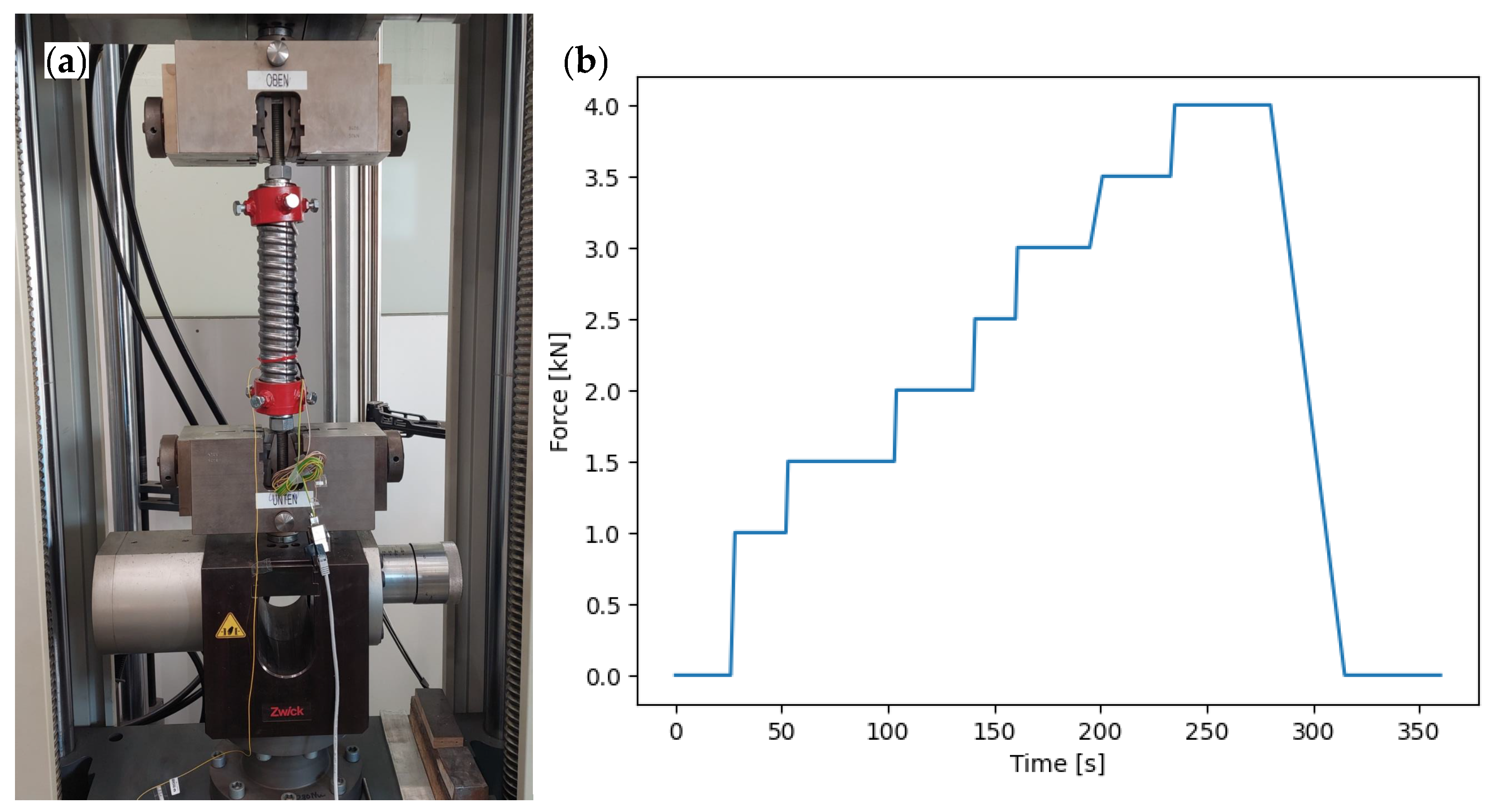
4.4. Test
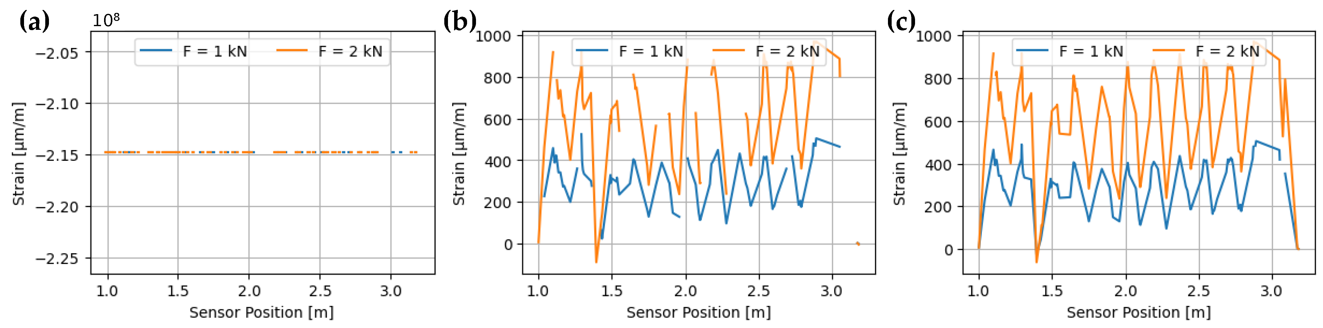
4.5. Results
4.6. Evaluation
5. Exposure to Environmental Conditions
5.1. Environment in a Concrete Lifecycle
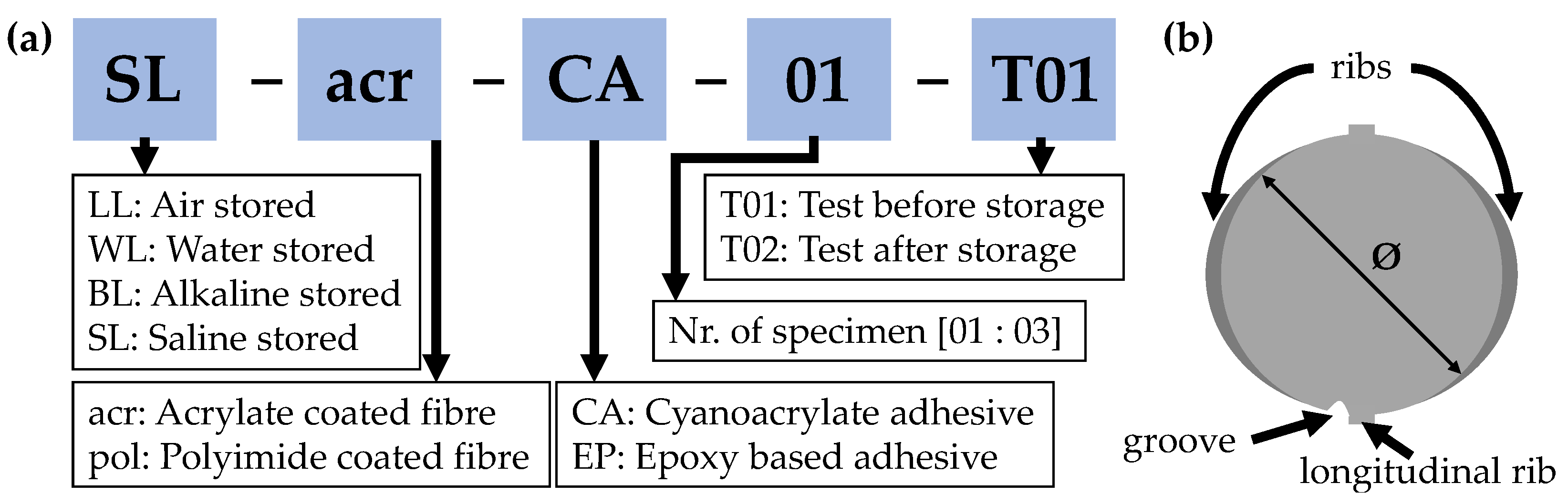
5.2. Basic Idea and Specimens
- Storage in air (LL)
- Storage in water (WL)
- Storage in alkaline environment (BL)
- Storage in saline (SL)
5.3. Theory
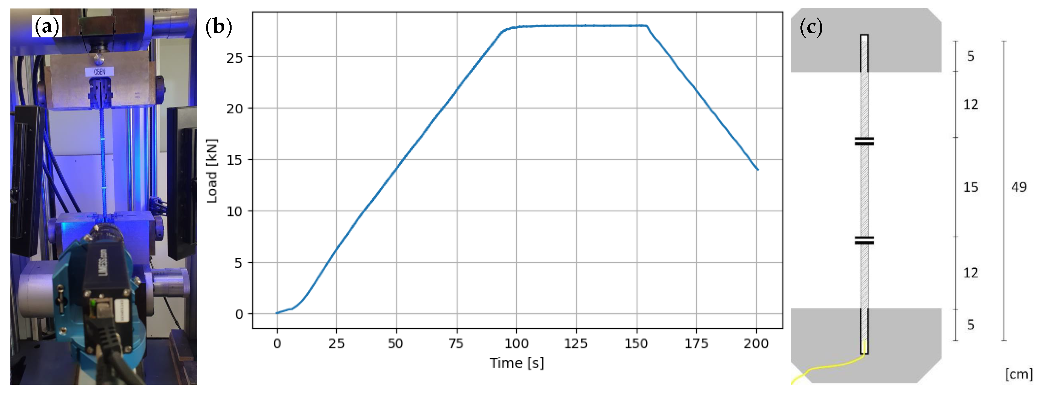
5.4. Test
5.5. Results
5.5.1. Pre-Processing of DFOS Data
- Gauge smoothed: The data obtained from measurements is smoothed in the direction of the sensor using gauges. This procedure ensures that the smoothed values of a measurement point in Figure 10d can deviate from the actual values (original) over time without eliminating large peaks. In a section taken at a specific point in time, the curve is significantly smoothed (see Figure 10e).
- Gauge and time smoothed: If both smoothing variants are executed together, the result is smoothing oriented in the time and sensor directions. The order of operations does not affect the results for the data sets used in this study.
5.5.2. Qualitative Results
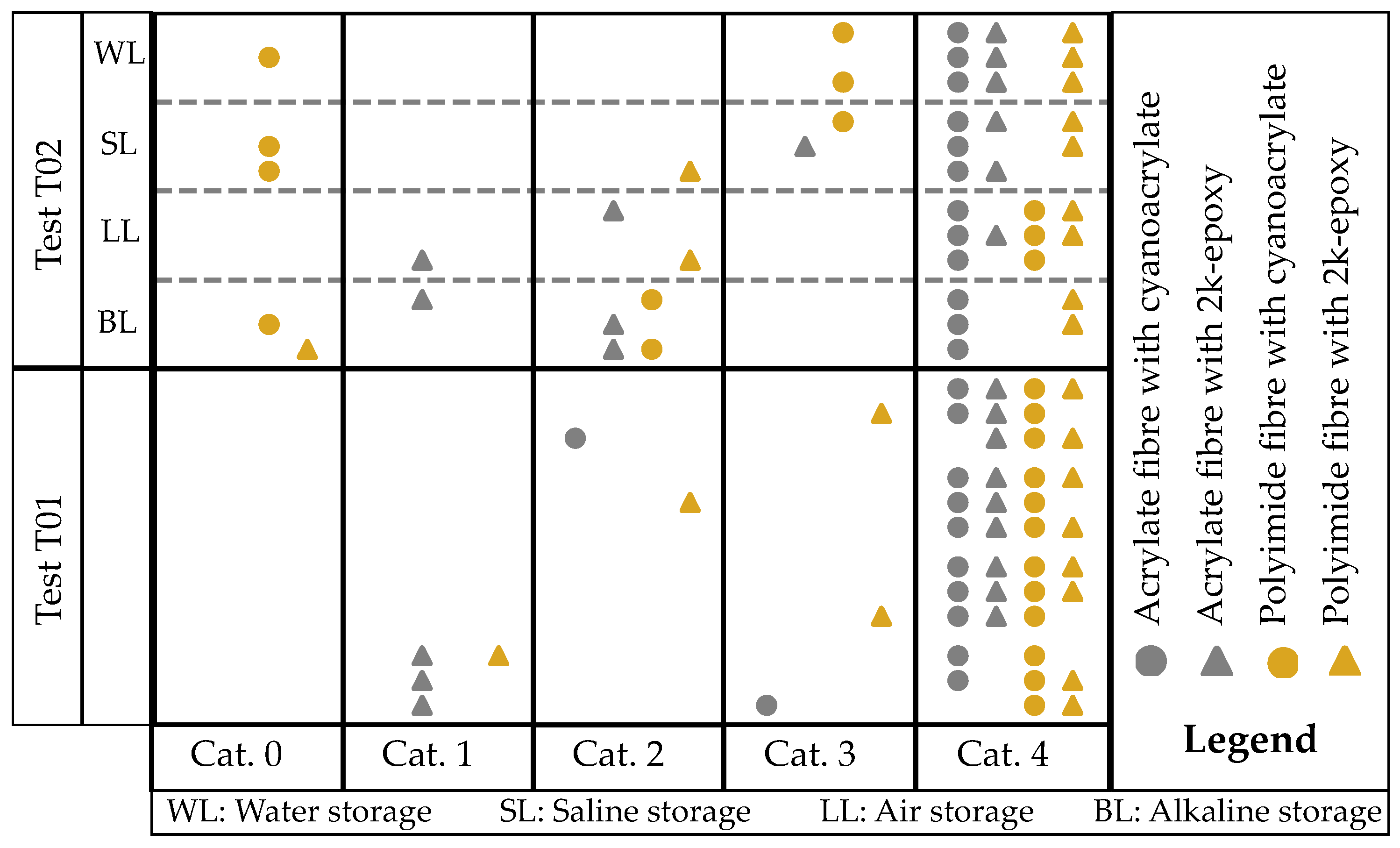
- Category 1: No measurement values available: It is important to distinguish whether no measurement data could be collected in both test runs or only in the second one. If no measurement data was collected in one run, it may indicate a faulty sensor rod. This could be due to damage caused during fabrication or during storage. As a result, the sensors no longer have a connection to the measuring device and are no longer recognised as sensors. These specimens are classified as subcategory 0. Category 1 includes all specimens recognised by the measuring device that only consist of dropouts and SRAs in the data of interest. It is depicted in Figure 12 (Cat. 1).
- Category 2: Measurement values with significant errors: This category contains data with significant anomalies, such as pronounced peaks and many dropouts. An example of this can be seen in Figure 12 (Cat. 2). The left graph clearly shows the strong peaks and the sensor failure after a certain time. In the right graph, the sensor failure can be seen in a medium time segment and SRAs in working segments. Loose contacts in the pigtail or splice points can cause issues with the measuring system’s ability to accurately record backscatter and transform it into strain.
- Category 3: Slightly erroneous measured values present: The measured values contain few anomalies, mostly SRAs or dropouts that are isolated in terms of time or location. This is illustrated in Figure 12 (Cat. 3) with two examples.
- Category 4: No abnormalities: In this case, the analysed measured values are free of errors. This is demonstrated in Figure 12 (Cat. 4). However, the quality of the curve, based on quantitative characteristics, such as noise or plausibility of the measured strains, has not yet been evaluated.
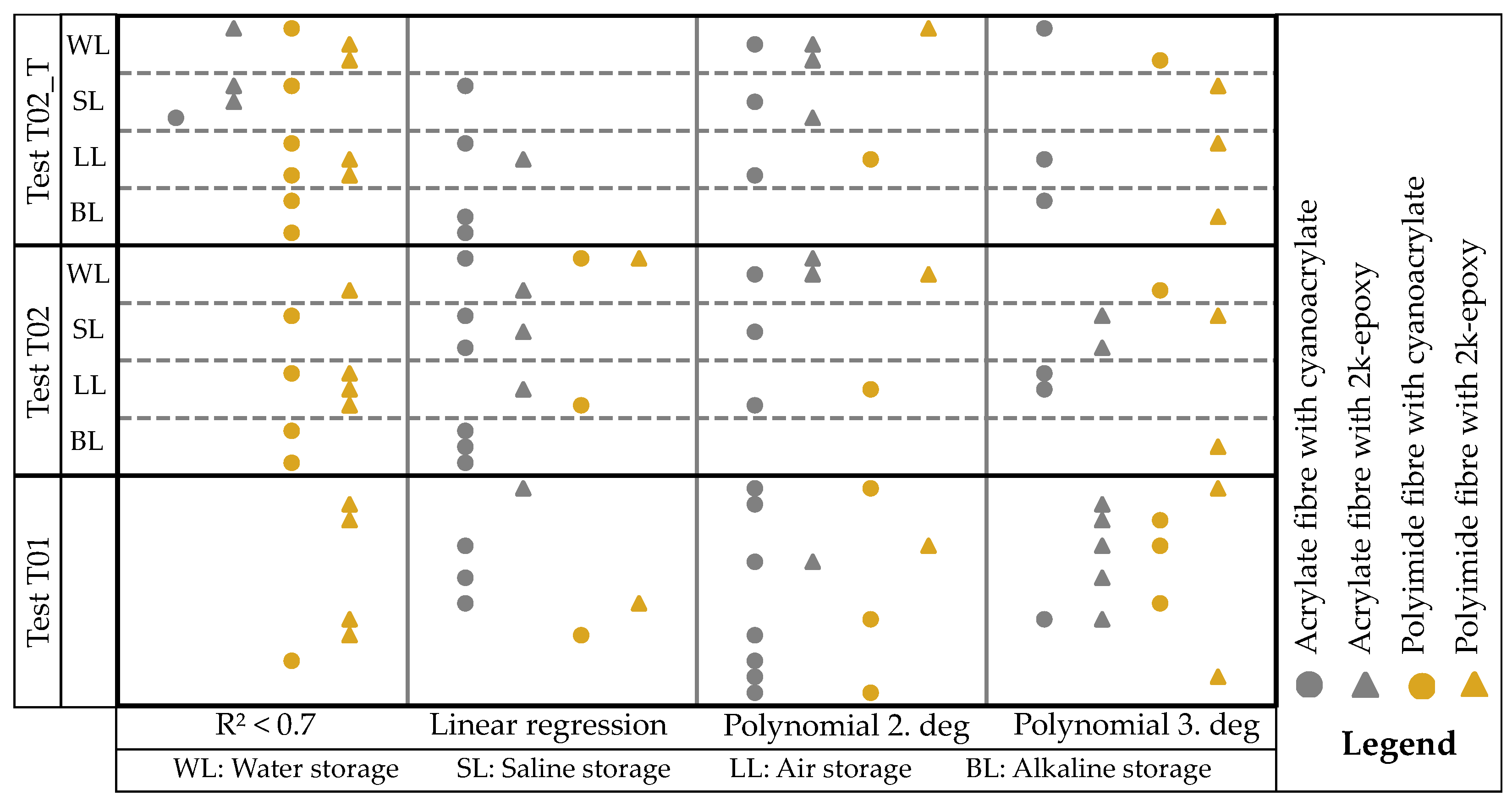
- If the are similar (relative standard deviation of the three values less than 5%), then the curve can be seen as a linear regression.
- If the values of the linear regression is significantly smaller than the of the polynomial regressions, these are compared. The measured values are categorised as 2nd degree polynomial regression if the following applies: . Otherwise it is categorised as 3rd degree polynomial regression.
- The coefficient of determination of the categorisation applies to the categorised curve.
- In general: A categorisation as ’bad regression’ applies if .
5.5.3. Quantitative Results
- Minimum/maximum values of the measured strains.
- Average value of the measured strains.
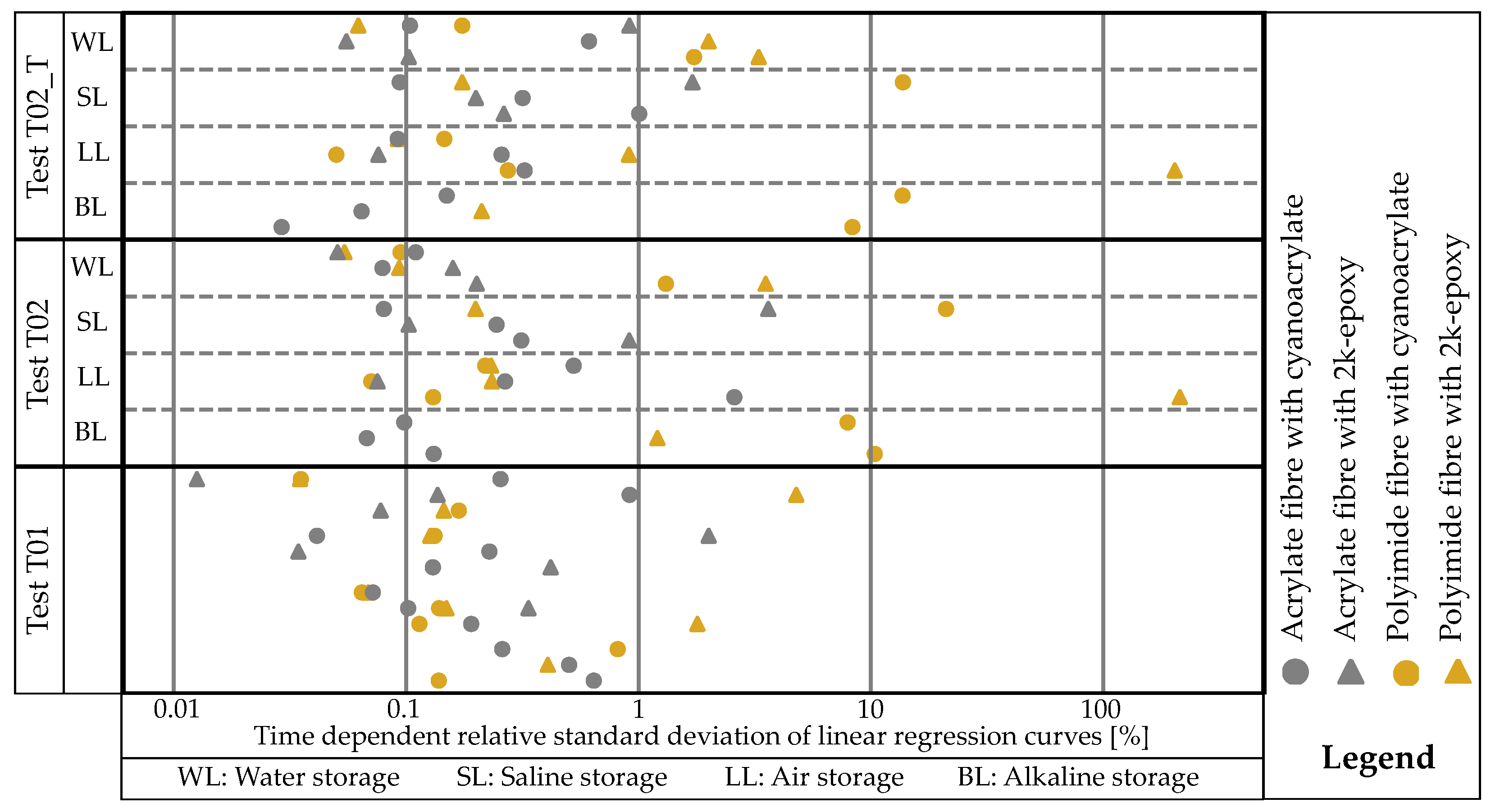
- Stability of the measurement over time using the regression curves.
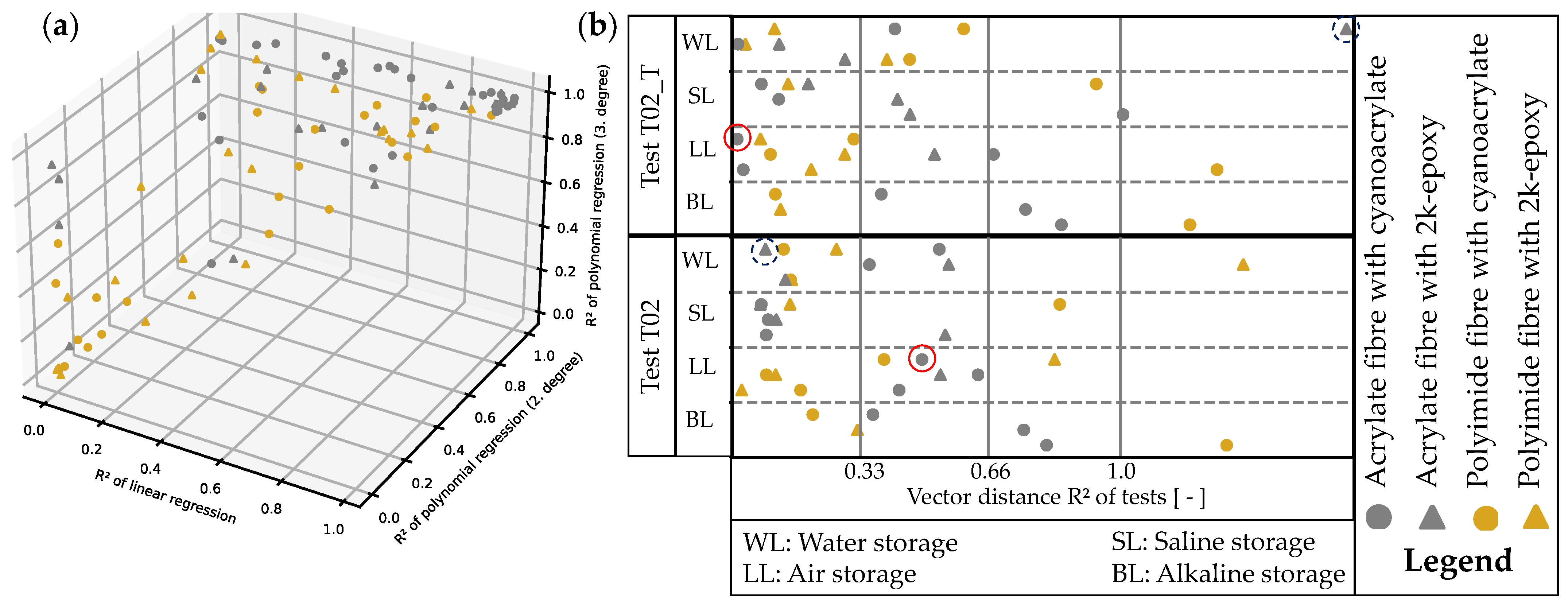
- Comparison of the measurements using the of the regressions.
5.6. Evaluation
6. Discussion of the Previous Experiments
7. Conclusions and Outlook
Author Contributions
Funding
Institutional Review Board Statement
Informed Consent Statement
Data Availability Statement
Acknowledgments
Conflicts of Interest
References
- Kenel, A.; Nellen, P.; Frank, A.; Marti, P. Reinforcing Steel Strains Measured by Bragg Grating Sensors. J. Mater. Civ. Eng. 2005, 17, 423–431. [Google Scholar] [CrossRef]
- Wu, Z.; Xu, B.; Hayashi, K.; Machida, A. Distributed optic fiber sensing for a full-scale PC girder strengthened with prestressed PBO sheets. Eng. Struct. 2006, 7, 1049–1059. [Google Scholar] [CrossRef]
- Bado, M.F.; Casas, J.R. A Review of Recent Distributed Optical Fiber Sensors Applications for Civil Engineering Structural Health Monitoring. Sensors 2021, 21, 1818. [Google Scholar] [CrossRef] [PubMed]
- Barrias, A.; Casas, J.R.; Villalba, S. A Review of Distributed Optical Fiber Sensors for Civil Engineering Applications. Sensors 2016, 16, 748. [Google Scholar] [CrossRef] [PubMed]
- Eberlein, D. Grundlagen der Lichtwellenleitertechnik, 1st ed.; Expert verlag Gmbh Tübingen: Tübingen, Germany, 2021; pp. 139–152. (In German) [Google Scholar]
- Wimmer, J.; Braml, T. Obtaining data from concrete structures. In Proceedings of the ISRERM 2022, Hannover, Germany, 4–7 September 2022; MS-04-027. pp. 83–90. [Google Scholar] [CrossRef]
- Galkovski, T.; Lemcherreq, Y.; Mata-Falcón, J.; Kaufmann, W. Fundamental Studies on the Use of Distributed Fibre Optical Sensing on Concrete and Reinforcing Bars. Sensors 2021, 21, 7643. [Google Scholar] [CrossRef] [PubMed]
- Mata-Falcón, J.; Haefliger, S.; Lee, M.; Galkovski, T.; Gehri, N. Combined application of distributed fibre optical and digital image correlation measurements to structural concrete experiments. Eng. Struct. 2020, 225, 111309. [Google Scholar] [CrossRef]
- Alj, I.; Quiertant, M.; Khadour, A.; Grando, Q.; Benzarti, K. Durability of Distributed Optical Fiber Sensors Used for SHM of Reinforced Concrete Structures. In Proceedings of the Structural Health Monitoring, Lancaster, PA, USA, 24–26 October 2018. [Google Scholar] [CrossRef]
- Bremer, K.; Alwis, L.S.M.; Zheng, Y.; Weigand, F.; Kuhne, M.; Helbig, R.; Roth, B. Durability of Functionalized Carbon Structures with Optical Fiber Sensors in a Highly Alkaline Concrete Environment. Appl. Sci. 2019, 9, 2476. [Google Scholar] [CrossRef]
- Kuwabara, T.; Katsuyama, Y. Polyetherimide coated optical silica glass fiber with high resistance to alkaline solution. In Proceedings of the OFC’89, Houston, TX, USA, 6–9 February 1989. [Google Scholar] [CrossRef]
- Habel, W.R.; Hofmann, D.; Hillemeier, B. Reinforcing Deformation measurements of mortars at early ages and of large concrete components on site by means of embedded fiber-optic microstrain sensors. Cem. Concr. Compos. 1997, 19, 81–102. [Google Scholar] [CrossRef]
- Bednarski, Ł.; Sieńko, R.; Howiacki, T.; Zuziak, K. The Smart Nervous System for Cracked Concrete Structures: Theory, Design, Research, and Field Proof of Monolithic DFOS-Based Sensors. Sensors 2022, 22, 8713. [Google Scholar] [CrossRef]
- Herbers, M.; Richter, B.; Gebauer, D.; Classen, M.; Marx, S. Crack monitoring on concrete structures: Comparison of various distributed fiber optic sensors with digital image correlation method. Struct. Concr. 2023, 24, 6123–6140. [Google Scholar] [CrossRef]
- Her, S.C.; Huang, C.Y. Effect of coating on the strain transfer of optical fiber sensors. Sensors 2011, 11, 6926–6941. [Google Scholar] [CrossRef] [PubMed]
- Kim, S.W.; Jeong, M.S.; Lee, I.; Kim, E.H.; Kwon, I.B.; Hwang, T.K. Determination of the maximum strains experienced by composite structures using metal coated optical fiber sensors. Compos. Sci. Technol. 2013, 78, 48–55. [Google Scholar] [CrossRef]
- Alj, I.; Quiertant, M.; Khadour, A.; Grando, Q.; Terrade, B.; Renaud, J.C.; Benzarti, K. Experimental and Numerical Investigation on the Strain Response of Distributed Optical Fiber Sensors Bonded to Concrete: Influence of the Adhesive Stiffness on Crack Monitoring Performance. Sensors 2020, 20, 5144. [Google Scholar] [CrossRef] [PubMed]
- Barrias, A.; Casas, J.R.; Villalba, S. Distributed optical fibre sensors in concrete structures: Performance of bonding adhesives and influence of spatial resolution. Struct. Control Health Monit. 2019, 26, 1–16. [Google Scholar] [CrossRef]
- Bado, M.F.; Casas, J.R.; Dey, A.; Berrocal, C.G. Distributed Optical Fiber Sensing Bonding Techniques Performance for Embedment inside Reinforced Concrete Structures. Sensors 2020, 20, 5788. [Google Scholar] [CrossRef]
- Gong, S.; Feng, X. Detection of grouting defects in prestressed tendon ducts using distributed fiber optic sensors. Struct. Health Monit. 2020, 19, 1273–1286. [Google Scholar] [CrossRef]
- Okubo, K.; Imai, M.; Sogabe, N.; Nakaue, S.; Chikiri, K.; Niwa, J. Development of the measuring method for PC-Tensile force distribution by optical fiber applicable to control of prestressing and maintenance of PC structures. J. JSCE E2 2020, 76, 41–54. (In Japanese) [Google Scholar] [CrossRef]
- Oikawa, M.; Nakaue, S.; Sogabe, N.; Imai, M. “SmART Strand” Prestressing Steel Strand with Optical Fiber Sensor for Tension Monitoring. In Proceedings of the 13th German-Japanese Bridge Symposium, Osaka, Japan, 29–30 August 2023; pp. 423–430. [Google Scholar]
- Gläser, C. Zustandsbewertung von Spannbetonbauwerken anhand von in Spannglieder integrierten ortsauflösenden Sensoren (smart tendons). In Proceedings of the 27 Münchener Massivbau Seminar, Munich, Germany, 24 November 2023; pp. 75–83. (In German) [Google Scholar] [CrossRef]
- Fischer, O.; Thoma, S.; Crepaz, S. Distributed fiber optic sensing for crack detection in concrete structures. Civ. Eng. Des. 2019, 1, 97–105. [Google Scholar] [CrossRef]
- Bassil, A.; Chapeleau, X.; Leduc, D.; Abraham, O. Concrete Crack Monitoring Using a Novel Strain Transfer Model for Distributed Fiber Optics Sensors. Sensors 2020, 20, 2220. [Google Scholar] [CrossRef]
- Alj, I.; Quiertant, M.; Khadour, A.; Grando, Q.; Benzarti, K. Environmental Durability of an Optical Fiber Cable Intended for Distributed Strain Measurements in Concrete Structures. Sensors 2021, 21, 141. [Google Scholar] [CrossRef]
- Howiacki, T.; Sieńko, R.; Bednarski, Ł; Zuziak, K. Crack Shape Coefficient: Comparison between Different DFOS Tools Embedded for Crack Monitoring in Concrete. Sensors 2023, 22, 566. [Google Scholar] [CrossRef] [PubMed]
- Winkler, M.; Monsberger, C.M.; Lienhart, W.; Vorwagner, A.; Kwapisz, M. Assessment of crack patterns along plain concrete tunnel linings using distributed fiber optic sensing. In Proceedings of the Fifth Conference on Smart Monitoring, Assessment and Rehabilitation of Civil Structures, Potsdam, Germany, 27–29 August 2019; Available online: https://data.smar-conferences.org/SMAR_2019_Proceedings/Inhalt/we.2.c.6.pdf. (accessed on 13 December 2023).
- Monsberger, C.M.; Lienhart, W. Distributed Fiber Optic Shape Sensing of Concrete Structures. Sensors 2021, 21, 6098. [Google Scholar] [CrossRef] [PubMed]
- Lemcherreq, Y.; Galkovski, T.; Mata-Falcón, J.; Kaufmann, W. Application of Distributed Fibre Optical Sensing in Reinforced Concrete Elements Subjected to Monotonic and Cyclic Loading. Sensors 2022, 22, 2023. [Google Scholar] [CrossRef] [PubMed]
- Bado, M.F.; Casas, J.R.; Barrias, A. Performance of Rayleigh-Based Distributed Optical Fiber Sensors Bonded to Reinforcing Bars in Bending. Sensors 2018, 18, 3125. [Google Scholar] [CrossRef] [PubMed]
- Berrocal, C.G.; Fernandez, I.; Bado, M.F.; Casas, J.R.; Rempling, R. Assessment and visualization of performance indicators of reinforced concrete beams by distributed optical fiber sensing. Struct. Health Monit. 2021, 20, 3309–3326. [Google Scholar] [CrossRef]
- Burger, H.; Tepho, T.; Fischer, O.; Schramm, N. Performance assessment of existing prestressed concrete bridges utilizing distributed optical fiber sensors. In Proceedings of the Eight IALCCE, Milan, Italy, 2–6 July 2023; pp. 3134–3141. [Google Scholar] [CrossRef]
- Haslbeck, M.; Böttcher, J.; Braml, T. An Uncertainty Model for Strain Gages Using Monte Carlo Methodology. Sensors 2023, 23, 8965. [Google Scholar] [CrossRef]
- Wimmer, J.; Braml, T. Permanent Structural Health Monitoring of a new prestressed concrete bridge. ce/papers 2023, 6, 691–700. [Google Scholar] [CrossRef]
- Wimmer, J.; Braml, T.; Martinez, R. Digitale Zwillinge für Brücken mittlerer Stützweite—Pilotprojekt Brücke Schwindegg—Teil 1: Sensorik. Beton Stahlbetonbau 2023, 118, 889–896. (In German) [Google Scholar] [CrossRef]
- Otterbach, L. Anbringen und Testen von Sensoren an Hüllrohren von Spanngliedern. Bachelor’s Thesis, University of the Bundeswehr Munich, Neubiberg, Germany, 2022. (In German). [Google Scholar]
- SUSPA DSI. Drawing No. L0003290-C SUSPA-DUCTS. Product sheet Langenfeld, Germany, 2010, Approved for production, unpublished.
- DIN EN 1992-2; Design of Concrete Structures—Part 1-1: General Rules and Rules for Buildings. Beuth Verlag GmbH: Berlin, Germany, 2010.
- DIN EN 1992-1-1; Design of Concrete Structures—Part 1-1: General Rules and Rules for Buildings. Beuth Verlag GmbH: Berlin, Germany, 2011.
- ETA-13/0839; SUSPA Strand DW. Austrian Institute of Construction Engineering: Vienna, Austria, 2021.
- DIN EN 10139; Cold Rolled Uncoated Low Carbon Steel Narrow Strip for Cold Forming—Technical Delivery Conditions. Beuth Verlag GmbH: Berlin, Germany, 2020.
- Richter, B.; Herbers, M.; Marx, S. Crack monitoring on concrete structures with distributed fiber optic sensors—Toward automated data evaluation and assessment. Struct. Concr. 2023, 25, 1465–1480. [Google Scholar] [CrossRef]
- Drake, D.; Sullivan, R.; Wilson, J. Distributed Strain Sensing from Different Optical Fiber Configurations. Inventions 2018, 3, 67. [Google Scholar] [CrossRef]
- DIN EN 206; Design of Concrete Structures—Part 1-1: General Rules and Rules for Buildings. Beuth Verlag GmbH: Berlin, Germany, 2021.
- Müller, H. Zum Einfluss des Klebstoffes und des Schutzmantels von auf Betonstabstählen geklebten Glasfasern auf deren Dauerhaftigkeit bei der Verteilten Dehnungsmessung. Master’s Thesis, University of the Bundeswehr Munich, Neubiberg, Germany, 2022. (In German). [Google Scholar]
- DIN 488-1; Reinforcing Steels—Part 1: Grades, Properties, Marking. Beuth Verlag GmbH: Berlin, Germany, 2009.
- DIN 488-2; Reinforcing Steels—Reinforcing Steel Bars. Beuth Verlag GmbH: Berlin, Germany, 2009.
- Pedregosa, F.; Varoquaux, G.; Gramfort, A.; Michel, V.; Thirion, B.; Grisel, O.; Blondel, M.; Prettenhofer, P.; Weiss, R.; Dubourg, V.; et al. Scikit-learn: Machine Learning in Python. JMLR 2011, 12, 2825–2830. [Google Scholar]
- Grefe, H.; Stammen, E.; Dilger, K.; Baudone, T.; Arutyunyan, G.; Baitinger, M. Using distributed fibreoptic sensing to monitor repaired structures reinforced with steel-patches. ce/papers 2023, 6, 1132–1136. [Google Scholar] [CrossRef]
- Qin, Z.; Qu, S.; Wang, Z.; Yang, W.; Li, S.; Liu, Z.; Xu, Y. A fully distributed fiber optic sensor for simultaneous relative humidity and temperature measurement with polyimide-coated polarization maintaining fiber. Sensors Actuators Chem. 2022, 373, 132699. [Google Scholar] [CrossRef]
- Thomas, P.J.; Hellevang, J.O. A high response polyimide fiber optic sensor for distributed humidity measurements. Sensors Actuators Chem. 2018, 270, 417–423. [Google Scholar] [CrossRef]
- Stajanca, P.; Hicke, K.; Krebber, K. Distributed Fiberoptic Sensor for Simultaneous Humidity and Temperature Monitoring Based on Polyimide-Coated Optical Fibers. Sensors 2019, 19, 5279. [Google Scholar] [CrossRef]


| Sensing Technology | Transducer Type | Sensing Range | Spatial Resolution | Main Measurands |
|---|---|---|---|---|
| Raman OTDR | distributed | 1–37 km | 1 cm–17 m | temperature |
| Brillouin OTDR | distributed | 20–50 km | ≈1 m | temperature, Strain |
| Brillouin OTDA | distributed | 150–200 km | 2 cm (2 km)–2 m (150 km) | temperature, strain |
| Rayleigh OFDR/DAS | distributed | 50–70 m | ≈1 mm | temperature, strain |
| FBG | quasi-distributed | ≈100 channels | 2 mm (Bragg length) | temperature, strain, displacement |
| Parameter | Duct Attributes | ||||||
|---|---|---|---|---|---|---|---|
| [mm] | 40 | 45 | … | 105 | 110 | 115 | 120 |
| [mm] | 26 | 26 | … | 26 | 24 | 24 | 24 |
| 0.171 | 0.155 | … | 0.073 | 0.065 | 0.062 | 0.060 | |
| Fibre | Polyimid | Acrylate | ||||
|---|---|---|---|---|---|---|
| Bonding | 2k Epoxy | Cyanoacrylate | 2k Epoxy | Cyanoacrylate | ||
| Figure 13 | Category | T02 | 1, 0, 2, 0, 9 | 4, 0, 2, 3, 3 | 0, 2, 3, 1, 6 | 0, 0, 0, 0, 12 |
| 0, 1, 2, 3, 4 | T01 | 0, 1, 1, 2, 8 | 0, 0, 0, 0, 12 | 0, 3, 0, 0, 9 | 0, 0, 1, 1, 10 | |
| Score category | 3 | 1 | 2 | 4 | ||
| Figure 15 | Regression type | T02_T | 4, 0, 1, 3 | 6, 0, 1, 1 | 3, 1, 3, 0 | 1, 4, 3, 3 |
| 0, lin, pol2, pol3 * | T02 | 4, 1, 1, 2 | 4, 2, 1, 1 | 0, 3, 2, 2 | 0, 6, 3, 2 | |
| T01 | 4, 1, 1, 2 | 1, 1, 3, 3 | 0, 1, 1, 5 | 0, 3, 7, 1 | ||
| Score regression type | 2 | 1 | 3 | 4 | ||
| Figure 16 | Range of | T02_T | 3, 3, 1, 1 | 2, 4, 0, 2 | 4, 2, 1, 0 | 10, 1, 0, 0 |
| measurement | T02 | 6, 1, 1, 0 | 2, 5, 0, 1 | 4, 2, 1, 0 | 9, 2, 0, 0 | |
| 100, 200, 300, + ** | T01 | 2, 5, 1, 0 | 6, 2, 0, 0 | 6, 1, 0, 0 | 10, 1, 0, 0 | |
| Score measurement range | 2 | 1 | 3 | 4 | ||
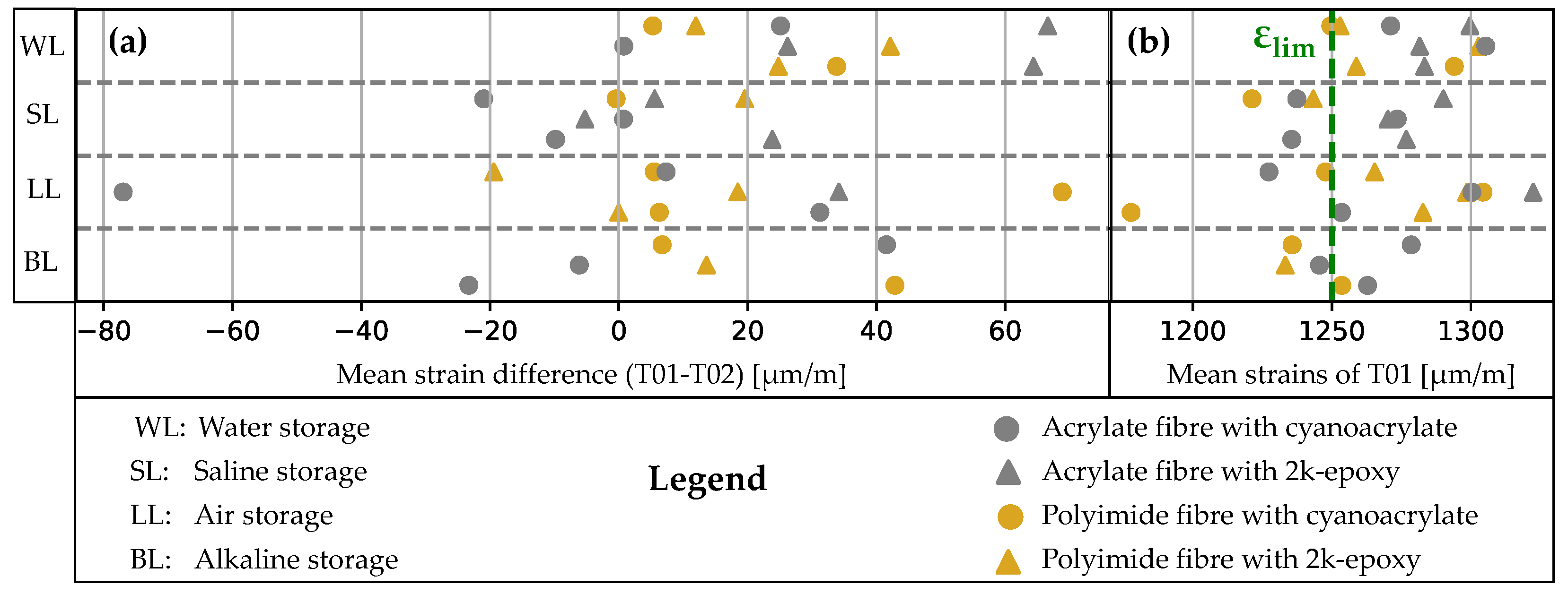
| Figure 17 | Mean strain difference T01−T02 | 6, 1, 1, 0 | 5, 1, 1, 1 | 2, 3, 0, 2 | 5, 4, 1, 1 | |
| ±20, ±40, ±60, ± *** | ||||||
| Score mean strain difference | 4 | 2 | 1 | 3 | ||
| Figure 18 | Standard deviation | T02_T | 2, 3, 2, 1 | 1, 3, 2, 2 | 2, 4, 1, 0 | 4, 6, 1, 0 |
| of linear regression | T02 | 2, 3, 2, 1 | 2, 2, 2, 2 | 2, 4, 1, 0 | 4, 6, 1, 0 | |
| 0.1, 1, 10, +% **** | T01 | 2, 4, 2, 0 | 2, 6, 0, 0 | 3, 3, 1, 0 | 2, 9, 0, 0 | |
| Score standard deviation | 2 | 1 | 3 | 4 | ||
| Figure 19 | Vector distance | T02 | 7, 1, 0, 0 | 3, 2, 1, 2 | 3, 3, 0, 1 | 5, 2, 3, 1 |
| 0.33, 0.66, 1, + ***** | T01 | 6, 0, 1, 1 | 5, 1, 1, 1 | 4, 3, 0, 0 | 3, 6, 2, 0 | |
| Score -Distance | 3 | 1 | 4 | 2 | ||
| Final Score ****** | 16 | 7 | 16 | 21 | ||
Disclaimer/Publisher’s Note: The statements, opinions and data contained in all publications are solely those of the individual author(s) and contributor(s) and not of MDPI and/or the editor(s). MDPI and/or the editor(s) disclaim responsibility for any injury to people or property resulting from any ideas, methods, instructions or products referred to in the content. |
© 2024 by the authors. Licensee MDPI, Basel, Switzerland. This article is an open access article distributed under the terms and conditions of the Creative Commons Attribution (CC BY) license (https://creativecommons.org/licenses/by/4.0/).
Share and Cite
Wimmer, J.; Braml, T. Investigation of the Robust Integration of Distributed Fibre Optic Sensors in Structural Concrete Components. Sensors 2024, 24, 6122. https://doi.org/10.3390/s24186122
Wimmer J, Braml T. Investigation of the Robust Integration of Distributed Fibre Optic Sensors in Structural Concrete Components. Sensors. 2024; 24(18):6122. https://doi.org/10.3390/s24186122
Chicago/Turabian StyleWimmer, Johannes, and Thomas Braml. 2024. "Investigation of the Robust Integration of Distributed Fibre Optic Sensors in Structural Concrete Components" Sensors 24, no. 18: 6122. https://doi.org/10.3390/s24186122
APA StyleWimmer, J., & Braml, T. (2024). Investigation of the Robust Integration of Distributed Fibre Optic Sensors in Structural Concrete Components. Sensors, 24(18), 6122. https://doi.org/10.3390/s24186122