
Hybrid Sparse Transformer and Wavelet Fusion-Based Deep Unfolding Network for Hyperspectral Snapshot Compressive Imaging


Abstract
1. Introduction
- We propose a novel method that hybridizes the sparse Transformer and wavelet fusion-based deep unfolding network for hyperspectral snapshot compressive imaging.
- To enhance the expressive capability of existing Transformer methods, we propose a sparse spatial–spectral Transformer. This approach uses sparse operations to avoid calculating correlations for irrelevant tokens during feature aggregation.
- To address the issue of information loss within and across stages of the DUN method, we design the wavelet-based intra-stage fusion module and wavelet-based inter-stage fusion module, respectively. These fusion modules utilize the characteristics of the wavelet transform to enhance HSI reconstruction.
2. Related Works
2.1. Model-Based Traditional Optimization Methods
2.2. Learning-Based Neural Network Methods
3. Method
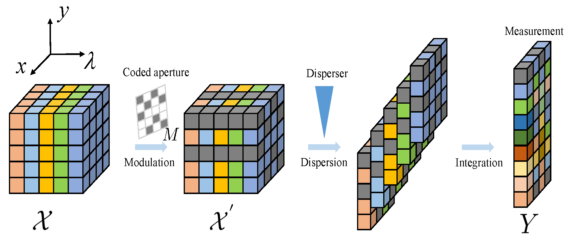
3.1. Preliminary
3.2. Overall Algorithm Framework
3.3. The Sparse Spatial–Spectral Transformer (SAET) Module
3.4. The Wavelet-Based Intra-Stage Fusion Module (WIntraFM)
3.5. The Wavelet-Based Inter-Stage Fusion Module (WInterFM)
4. Experimental Results
4.1. Experiment Setup
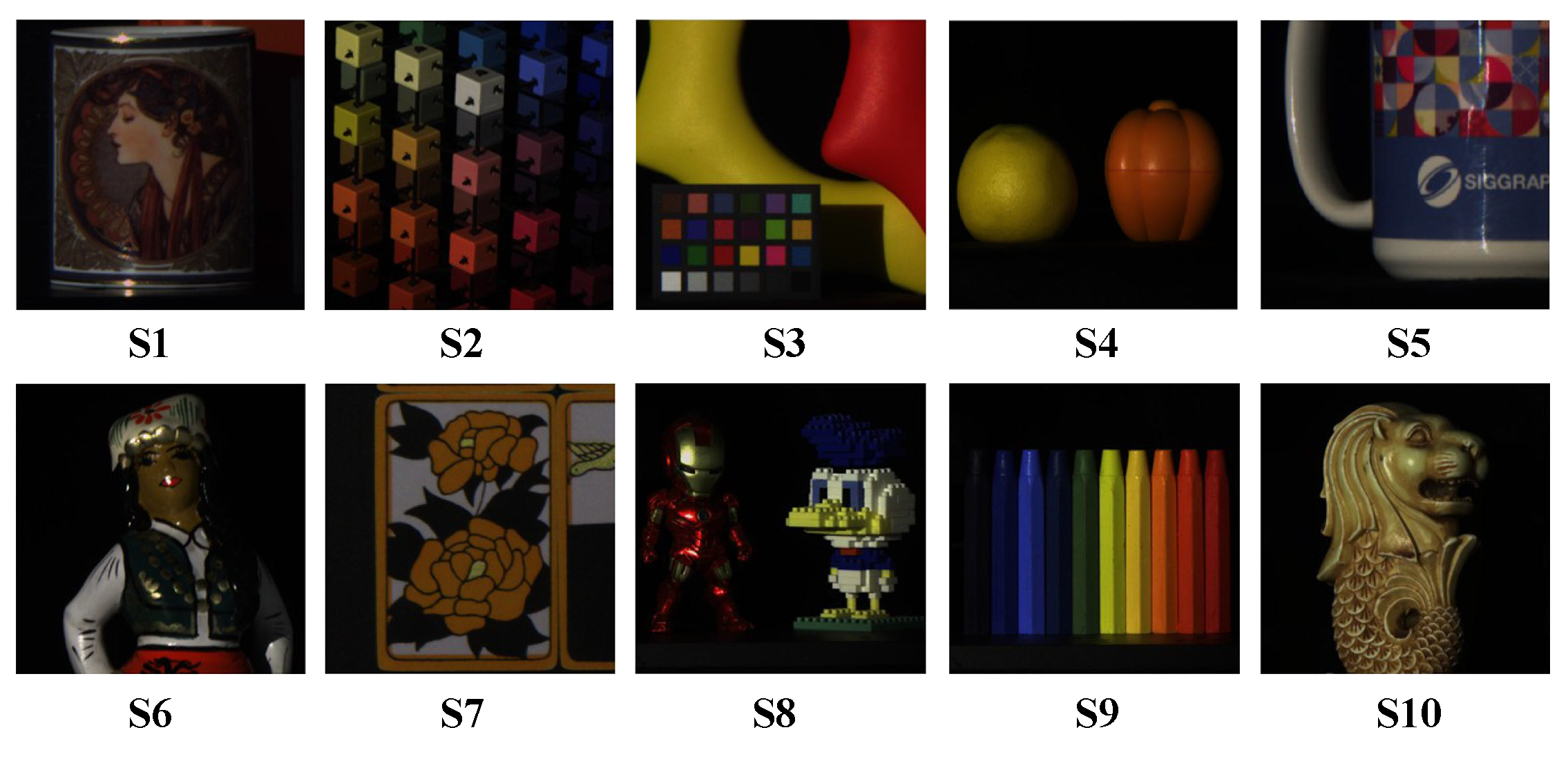
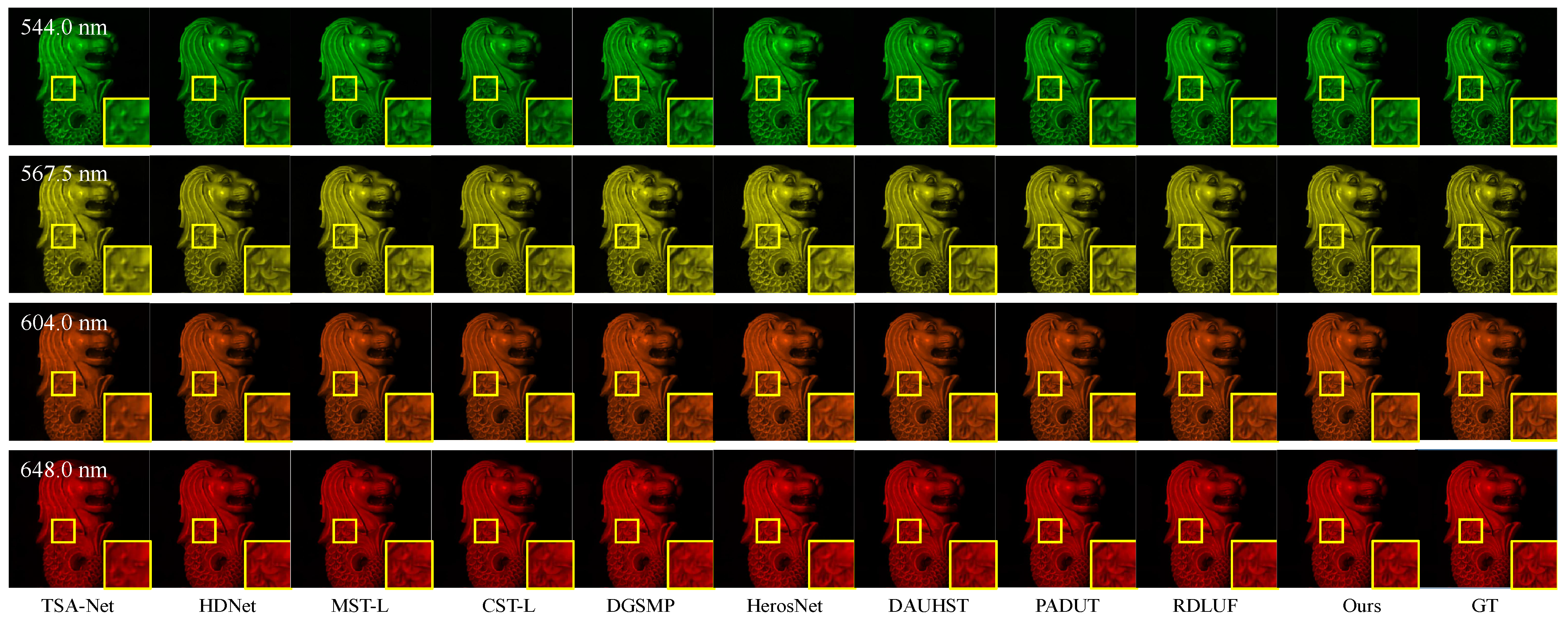
4.2. Simulation Results on CAVE and KAIST
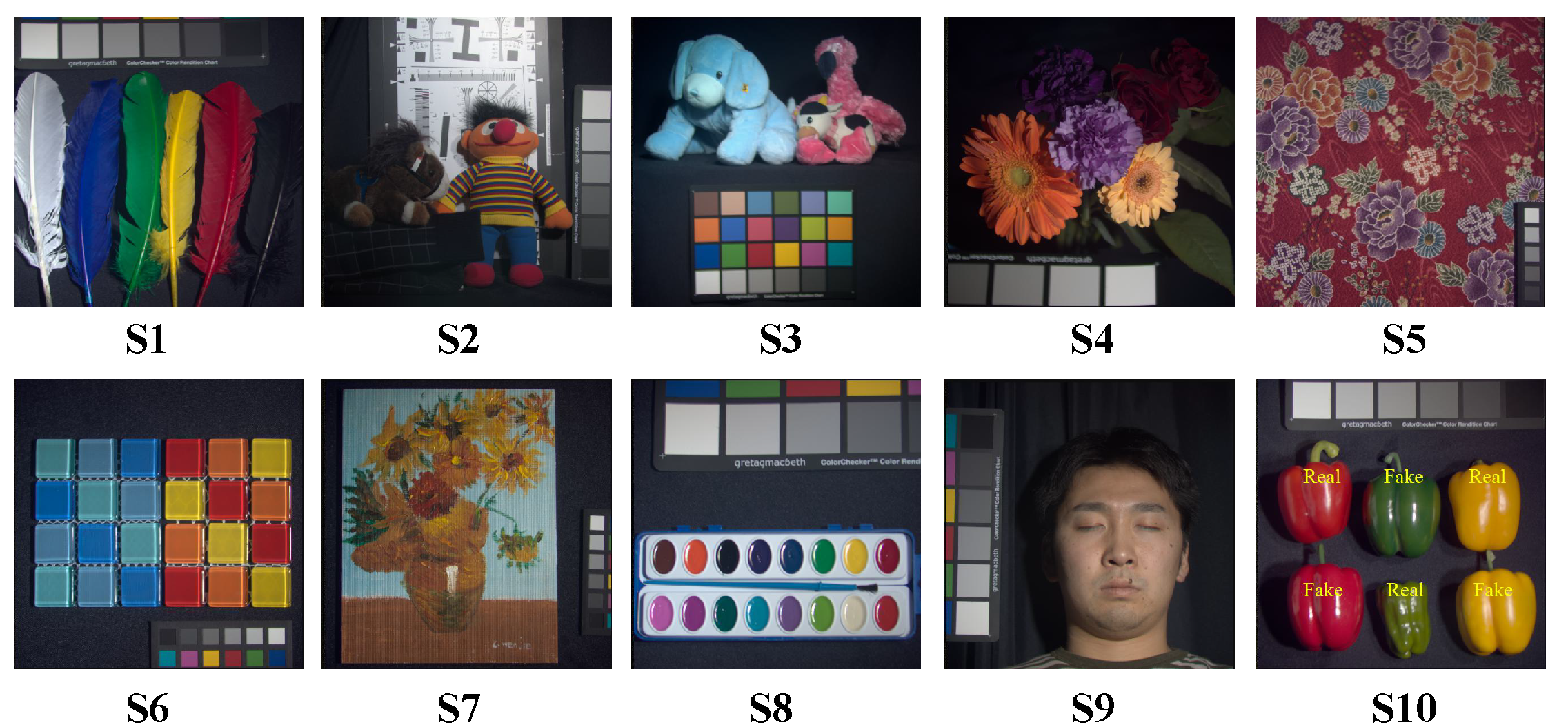
4.3. Simulation Results on ARAD_1K
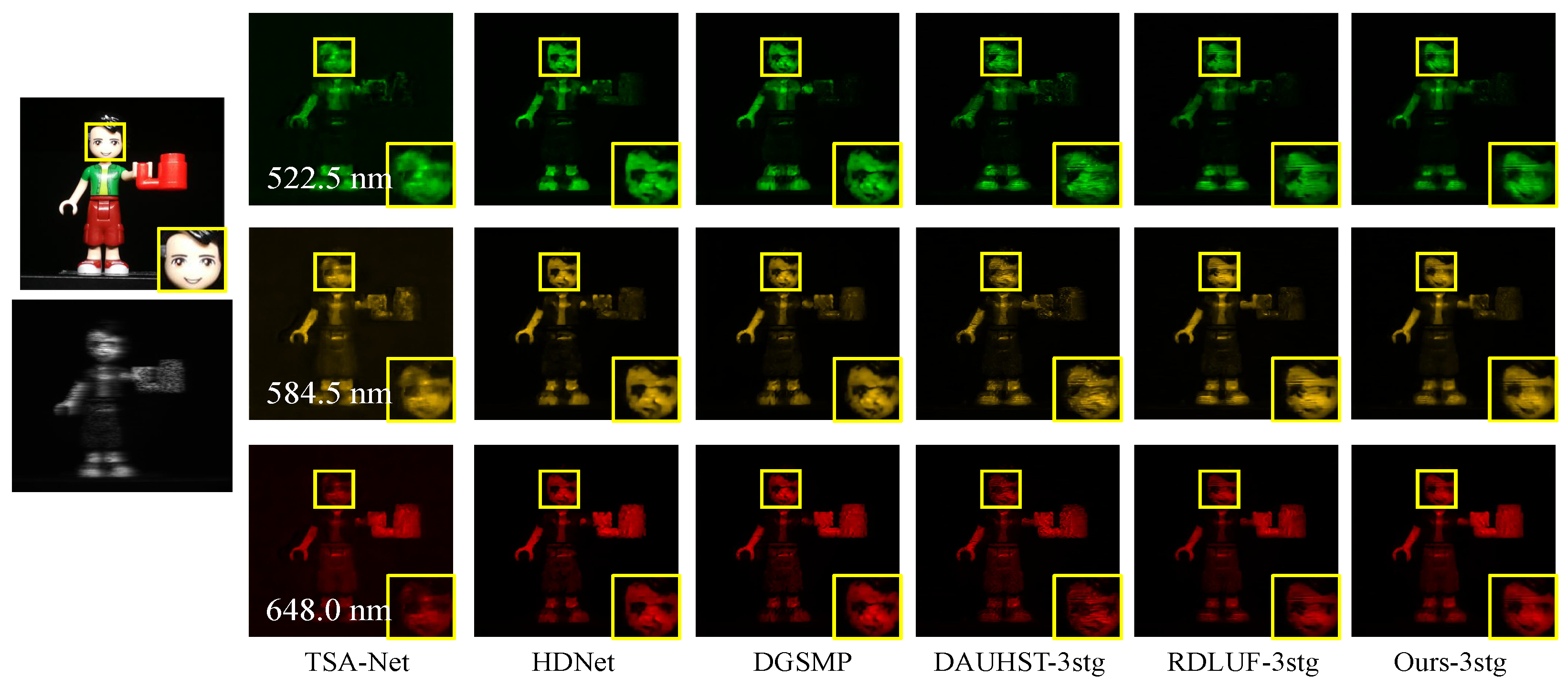
4.4. Real Data Results
4.5. Ablation Study
5. Conclusions
Author Contributions
Funding
Institutional Review Board Statement
Informed Consent Statement
Data Availability Statement
Conflicts of Interest
References
- Pan, Z.; Healey, G.; Prasad, M.; Tromberg, B. Face recognition in hyperspectral images. IEEE Trans. Pattern Anal. Mach. Intell. 2003, 25, 1552–1560. [Google Scholar]
- Huang, Y.; Peng, J.; Sun, W.; Chen, N.; Du, Q.; Ning, Y.; Su, H. Two-branch attention adversarial domain adaptation network for hyperspectral image classification. IEEE Trans. Geosci. Remote Sens. 2022, 60, 1–13. [Google Scholar] [CrossRef]
- Zhu, L.; Wu, J.; Biao, W.; Liao, Y.; Gu, D. Spectralmae: Spectral masked autoencoder for hyperspectral remote sensing image reconstruction. Sensors 2023, 23, 3728. [Google Scholar] [CrossRef]
- Wang, X.; Chen, J.; Wei, Q.; Richard, C. Hyperspectral image super-resolution via deep prior regularization with parameter estimation. IEEE Trans. Circuits Syst. Video Technol. 2021, 32, 1708–1723. [Google Scholar] [CrossRef]
- Liu, S.; Li, Z.; Wang, G.; Qiu, X.; Liu, T.; Cao, J.; Zhang, D. Spectral–Spatial Feature Fusion for Hyperspectral Anomaly Detection. Sensors 2024, 24, 1652. [Google Scholar] [CrossRef]
- He, C.; Wei, Y.; Guo, K.; Han, H. Removal of Mixed Noise in Hyperspectral Images Based on Subspace Representation and Nonlocal Low-Rank Tensor Decomposition. Sensors 2024, 24, 327. [Google Scholar] [CrossRef]
- Xie, Y.; Liu, C.; Liu, S.; Song, W.; Fan, X. Snapshot imaging spectrometer based on pixel-level filter array (PFA). Sensors 2021, 21, 2289. [Google Scholar] [CrossRef]
- Cao, X.; Yue, T.; Lin, X.; Lin, S.; Yuan, X.; Dai, Q.; Carin, L.; Brady, D.J. Computational snapshot multispectral cameras: Toward dynamic capture of the spectral world. IEEE Signal Process. Mag. 2016, 33, 95–108. [Google Scholar] [CrossRef]
- Wagadarikar, A.; John, R.; Willett, R.; Brady, D. Single disperser design for coded aperture snapshot spectral imaging. Appl. Optics 2008, 47, B44–B51. [Google Scholar] [CrossRef]
- Song, L.; Wang, L.; Kim, M.H.; Huang, H. High-accuracy image formation model for coded aperture snapshot spectral imaging. IEEE Trans. Comput. Imag. 2022, 8, 188–200. [Google Scholar] [CrossRef]
- Donoho, D.L. Compressed sensing. IEEE Trans. Inf. Theory 2006, 52, 1289–1306. [Google Scholar] [CrossRef]
- Yuan, X. Generalized alternating projection based total variation minimization for compressive sensing. In Proceedings of the 2016 IEEE International Conference on Image Processing (ICIP), Phoenix, AZ, USA, 25–28 September 2016; pp. 2539–2543. [Google Scholar]
- Lin, X.; Liu, Y.; Wu, J.; Dai, Q. Spatial-spectral encoded compressive hyperspectral imaging. ACM Trans. Graph. 2014, 33, 1–11. [Google Scholar] [CrossRef]
- Kittle, D.; Choi, K.; Wagadarikar, A.; Brady, D.J. Multiframe image estimation for coded aperture snapshot spectral imagers. Appl. Optics 2010, 49, 6824–6833. [Google Scholar] [CrossRef] [PubMed]
- García-Sánchez, I.; Fresnedo, Ó.; González-Coma, J.P.; Castedo, L. Coded aperture hyperspectral image reconstruction. Sensors 2021, 21, 6551. [Google Scholar] [CrossRef]
- Xu, Y.; Wu, Z.; Chanussot, J.; Wei, Z. Hyperspectral computational imaging via collaborative Tucker3 tensor decomposition. IEEE Trans. Circuits Syst. Video Technol. 2020, 31, 98–111. [Google Scholar] [CrossRef]
- Yang, J.; Liao, X.; Yuan, X.; Llull, P.; Brady, D.J.; Sapiro, G.; Carin, L. Compressive sensing by learning a Gaussian mixture model from measurements. IEEE Trans. Image Process. 2014, 24, 106–119. [Google Scholar] [CrossRef]
- Liu, Y.; Yuan, X.; Suo, J.; Brady, D.J.; Dai, Q. Rank minimization for snapshot compressive imaging. IEEE Trans. Pattern Anal. Mach. Intell. 2018, 41, 2990–3006. [Google Scholar] [CrossRef]
- Zhang, S.; Huang, H.; Fu, Y. Fast parallel implementation of dual-camera compressive hyperspectral imaging system. IEEE Trans. Circuits Syst. Video Technol. 2018, 29, 3404–3414. [Google Scholar] [CrossRef]
- He, W.; Yao, Q.; Li, C.; Yokoya, N.; Zhao, Q.; Zhang, H.; Zhang, L. Non-local meets global: An iterative paradigm for hyperspectral image restoration. IEEE Trans. Pattern Anal. Mach. Intell. 2020, 44, 2089–2107. [Google Scholar] [CrossRef]
- Sun, Y.; Yang, Y.; Liu, Q.; Kankanhalli, M. Unsupervised spatial-spectral network learning for hyperspectral compressive snapshot reconstruction. IEEE Trans. Geosci. Remote Sens. 2021, 60, 1–14. [Google Scholar] [CrossRef]
- Xu, P.; Liu, L.; Jia, Y.; Zheng, H.; Xu, C.; Xue, L. A Refinement Boosted and Attention Guided Deep FISTA Reconstruction Framework for Compressive Spectral Imaging. IEEE Trans. Geosci. Remote Sens. 2023, 61, 1–12. [Google Scholar] [CrossRef]
- Miao, X.; Yuan, X.; Pu, Y.; Athitsos, V. l-net: Reconstruct hyperspectral images from a snapshot measurement. In Proceedings of the 2019 IEEE/CVF International Conference on Computer Vision (ICCV), Seoul, Republic of Korea, 27 October–2 November 2019; pp. 4059–4069. [Google Scholar]
- Meng, Z.; Ma, J.; Yuan, X. End-to-end low cost compressive spectral imaging with spatial-spectral self-attention. In Proceedings of the European Conference on Computer Vision, Glasgow, UK, 23–28 August 2020; Springer: Cham, Switzerland, 2020; pp. 187–204. [Google Scholar]
- Cai, Y.; Lin, J.; Hu, X.; Wang, H.; Yuan, X.; Zhang, Y.; Timofte, R.; Van Gool, L. Mask-guided spectral-wise transformer for efficient hyperspectral image reconstruction. In Proceedings of the 2022 IEEE/CVF Conference on Computer Vision and Pattern Recognition (CVPR), New Orleans, LA, USA, 18–24 June 2022; pp. 17502–17511. [Google Scholar]
- Hu, X.; Cai, Y.; Lin, J.; Wang, H.; Yuan, X.; Zhang, Y.; Timofte, R.; Van Gool, L. Hdnet: High-resolution dual-domain learning for spectral compressive imaging. In Proceedings of the 2022 IEEE/CVF Conference on Computer Vision and Pattern Recognition (CVPR), New Orleans, LA, USA, 18–24 June 2022; pp. 17542–17551. [Google Scholar]
- Cai, Y.; Lin, J.; Hu, X.; Wang, H.; Yuan, X.; Zhang, Y.; Timofte, R.; Van Gool, L. Coarse-to-fine sparse transformer for hyperspectral image reconstruction. In Proceedings of the European Conference on Computer Vision, Tel Aviv, Israel, 23–27 October 2022; Springer: Cham, Switzerland, 2022; pp. 686–704. [Google Scholar]
- Cheng, Z.; Chen, B.; Lu, R.; Wang, Z.; Zhang, H.; Meng, Z.; Yuan, X. Recurrent neural networks for snapshot compressive imaging. IEEE Trans. Pattern Anal. Mach. Intell. 2022, 45, 2264–2281. [Google Scholar] [CrossRef] [PubMed]
- Zheng, S.; Liu, Y.; Meng, Z.; Qiao, M.; Tong, Z.; Yang, X.; Han, S.; Yuan, X. Deep plug-and-play priors for spectral snapshot compressive imaging. Photonics Res. 2021, 9, B18–B29. [Google Scholar] [CrossRef]
- Meng, Z.; Yu, Z.; Xu, K.; Yuan, X. Self-supervised neural networks for spectral snapshot compressive imaging. In Proceedings of the 2021 IEEE/CVF International Conference on Computer Vision (ICCV), Montreal, QC, Canada, 10–17 October 2021; pp. 2622–2631. [Google Scholar]
- Qiu, H.; Wang, Y.; Meng, D. Effective snapshot compressive-spectral imaging via deep denoising and total variation priors. In Proceedings of the 2021 IEEE/CVF Conference on Computer Vision and Pattern Recognition (CVPR), Nashville, TN, USA, 20–25 June 2021; pp. 9127–9136. [Google Scholar]
- Chen, Y.; Gui, X.; Zeng, J.; Zhao, X.L.; He, W. Combining low-rank and deep plug-and-play priors for snapshot compressive imaging. IEEE Trans. Neural Netw. Learn. Syst. 2023, 1–13. [Google Scholar] [CrossRef] [PubMed]
- Chen, Y.; Lai, W.; He, W.; Zhao, X.L.; Zeng, J. Hyperspectral compressive snapshot reconstruction via coupled low-rank subspace representation and self-supervised deep network. IEEE Trans. Image Process. 2024, 33, 926–941. [Google Scholar] [CrossRef]
- Meng, Z.; Jalali, S.; Yuan, X. Gap-net for snapshot compressive imaging. arXiv 2020, arXiv:2012.08364. [Google Scholar]
- Ma, J.; Liu, X.Y.; Shou, Z.; Yuan, X. Deep tensor admm-net for snapshot compressive imaging. In Proceedings of the 2019 IEEE/CVF International Conference on Computer Vision (ICCV), Seoul, Republic of Korea, 27 October–2 November 2019; pp. 10223–10232. [Google Scholar]
- Wang, L.; Sun, C.; Fu, Y.; Kim, M.H.; Huang, H. Hyperspectral image reconstruction using a deep spatial-spectral prior. In Proceedings of the 2019 IEEE/CVF Conference on Computer Vision and Pattern Recognition (CVPR), Long Beach, CA, USA, 15–20 June 2019; pp. 8032–8041. [Google Scholar]
- Wang, L.; Sun, C.; Zhang, M.; Fu, Y.; Huang, H. Dnu: Deep non-local unrolling for computational spectral imaging. In Proceedings of the 2020 IEEE/CVF Conference on Computer Vision and Pattern Recognition (CVPR), Seattle, WA, USA, 13–19 June 2020; pp. 1661–1671. [Google Scholar]
- Zhang, S.; Wang, L.; Zhang, L.; Huang, H. Learning tensor low-rank prior for hyperspectral image reconstruction. In Proceedings of the 2021 IEEE/CVF Conference on Computer Vision and Pattern Recognition (CVPR), Nashville, TN, USA, 20–25 June 2021; pp. 12006–12015. [Google Scholar]
- Huang, T.; Dong, W.; Yuan, X.; Wu, J.; Shi, G. Deep gaussian scale mixture prior for spectral compressive imaging. In Proceedings of the 2021 IEEE/CVF Conference on Computer Vision and Pattern Recognition (CVPR), Nashville, TN, USA, 20–25 June 2021; pp. 16216–16225. [Google Scholar]
- Huang, T.; Yuan, X.; Dong, W.; Wu, J.; Shi, G. Deep Gaussian Scale Mixture Prior for Image Reconstruction. IEEE Trans. Pattern Anal. Mach. Intell. 2023, 45, 10778–10794. [Google Scholar] [CrossRef]
- Wang, L.; Wu, Z.; Zhong, Y.; Yuan, X. Snapshot spectral compressive imaging reconstruction using convolution and contextual Transformer. Photonics Res. 2022, 10, 1848–1858. [Google Scholar] [CrossRef]
- Zhang, X.; Zhang, Y.; Xiong, R.; Sun, Q.; Zhang, J. HerosNet: Hyperspectral Explicable Reconstruction and Optimal Sampling Deep Network for Snapshot Compressive Imaging. In Proceedings of the 2022 IEEE/CVF Conference on Computer Vision and Pattern Recognition (CVPR), New Orleans, LA, USA, 18–24 June 2022; pp. 17532–17541. [Google Scholar]
- Ying, Y.; Wang, J.; Shi, Y.; Yin, B. Dual-Domain Feature Learning and Memory-Enhanced Unfolding Network for Spectral Compressive Imaging. In Proceedings of the 2023 IEEE International Conference on Multimedia and Expo (ICME), Brisbane, Australia, 10–14 July 2023; pp. 1589–1594. [Google Scholar]
- Cai, Y.; Lin, J.; Wang, H.; Yuan, X.; Ding, H.; Zhang, Y.; Timofte, R.; Gool, L.V. Degradation-aware unfolding half-shuffle transformer for spectral compressive imaging. Adv. Neural Inf. Process. Syst. 2022, 35, 37749–37761. [Google Scholar]
- Li, M.; Fu, Y.; Liu, J.; Zhang, Y. Pixel Adaptive Deep Unfolding Transformer for Hyperspectral Image Reconstruction. In Proceedings of the 2023 IEEE/CVF International Conference on Computer Vision (ICCV), Paris, France, 1–6 October 2023; pp. 12959–12968. [Google Scholar]
- Dong, Y.; Gao, D.; Qiu, T.; Li, Y.; Yang, M.; Shi, G. Residual degradation learning unfolding framework with mixing priors across spectral and spatial for compressive spectral imaging. In Proceedings of the 2023 IEEE/CVF Conference on Computer Vision and Pattern Recognition (CVPR), Vancouver, BC, Canada, 17–24 June 2023; pp. 22262–22271. [Google Scholar]
- Yang, J.; Lin, T.; Liu, F.; Xiao, L. Learning Degradation-Aware Deep Prior for Hyperspectral Image Reconstruction. IEEE Trans. Geosci. Remote Sens. 2023, 61, 1–15. [Google Scholar] [CrossRef]
- Xu, P.; Liu, L.; Zheng, H.; Yuan, X.; Xu, C.; Xue, L. Degradation-aware dynamic fourier-based network for spectral compressive imaging. IEEE Trans. Multimed. 2023, 26, 2838–2850. [Google Scholar] [CrossRef]
- Qin, X.; Quan, Y.; Ji, H. Enhanced deep unrolling networks for snapshot compressive hyperspectral imaging. Neural Netw. 2024, 174, 106250. [Google Scholar] [CrossRef] [PubMed]
- Zhang, J.; Zeng, H.; Cao, J.; Chen, Y.; Yu, D.; Zhao, Y.P. Dual Prior Unfolding for Snapshot Compressive Imaging. In Proceedings of the 2024 IEEE/CVF Conference on Computer Vision and Pattern Recognition (CVPR), Seattle, WA, USA, 16–22 June 2024; pp. 25742–25752. [Google Scholar]
- Dosovitskiy, A.; Beyer, L.; Kolesnikov, A.; Weissenborn, D.; Zhai, X.; Unterthiner, T.; Dehghani, M.; Minderer, M.; Heigold, G.; Gelly, S.; et al. An image is worth 16x16 words: Transformers for image recognition at scale. arXiv 2020, arXiv:2010.11929. [Google Scholar]
- Fu, Z.; Fu, Z.; Liu, Q.; Cai, W.; Wang, Y. Sparsett: Visual tracking with sparse transformers. arXiv 2022, arXiv:2205.03776. [Google Scholar]
- Chen, X.; Li, H.; Li, M.; Pan, J. Learning a sparse transformer network for effective image deraining. In Proceedings of the 2023 IEEE/CVF Conference on Computer Vision and Pattern Recognition (CVPR), Vancouver, BC, Canada, 17–24 June 2023; pp. 5896–5905. [Google Scholar]
- Zhou, H.; Lian, Y.; Li, J.; Liu, Z.; Cao, X.; Ma, C. Supervised-unsupervised combined transformer for spectral compressive imaging reconstruction. Opt. Lasers Eng. 2024, 175, 108030. [Google Scholar] [CrossRef]
- Li, J.; Zheng, K.; Gao, L.; Ni, L.; Huang, M.; Chanussot, J. Model-informed Multi-stage Unsupervised Network for Hyperspectral Image Super-resolution. IEEE Trans. Geosci. Remote Sens. 2024, 62, 5516117. [Google Scholar]
- Cao, X.; Lian, Y.; Wang, K.; Ma, C.; Xu, X. Unsupervised hybrid network of transformer and CNN for blind hyperspectral and multispectral image fusion. IEEE Trans. Geosci. Remote Sens. 2024, 62, 5507615. [Google Scholar] [CrossRef]
- Ma, W.; Pan, Z.; Guo, J.; Lei, B. Achieving super-resolution remote sensing images via the wavelet transform combined with the recursive res-net. IEEE Trans. Geosci. Remote Sens. 2019, 57, 3512–3527. [Google Scholar] [CrossRef]
- Dong, J.; Pan, J.; Yang, Z.; Tang, J. Multi-scale residual low-pass filter network for image deblurring. In Proceedings of the 2023 IEEE/CVF International Conference on Computer Vision (ICCV), Paris, France, 1–6 October 2023; pp. 12345–12354. [Google Scholar]
- Torrence, C.; Compo, G.P. A practical guide to wavelet analysis. Bull. Am. Meteorol. Soc. 1998, 79, 61–78. [Google Scholar] [CrossRef]
- Liao, X.; Li, H.; Carin, L. Generalized alternating projection for weighted-2,1 minimization with applications to model-based compressive sensing. SIAM J. Imaging Sci. 2014, 7, 797–823. [Google Scholar] [CrossRef]
- Boyd, S.; Parikh, N.; Chu, E.; Peleato, B.; Eckstein, J. Distributed optimization and statistical learning via the alternating direction method of multipliers. Found. Trends Mach. Learn. 2011, 3, 1–122. [Google Scholar] [CrossRef]
- Liu, Z.; Lin, Y.; Cao, Y.; Hu, H.; Wei, Y.; Zhang, Z.; Lin, S.; Guo, B. Swin transformer: Hierarchical vision transformer using shifted windows. In Proceedings of the 2021 IEEE/CVF International Conference on Computer Vision (ICCV), Montreal, QC, Canada, 10–17 October 2021; pp. 10012–10022. [Google Scholar]
- Beck, A.; Teboulle, M. A fast iterative shrinkage-thresholding algorithm for linear inverse problems. SIAM J. Imaging Sci. 2009, 2, 183–202. [Google Scholar] [CrossRef]
- Park, J.I.; Lee, M.H.; Grossberg, M.D.; Nayar, S.K. Multispectral imaging using multiplexed illumination. In Proceedings of the 2007 IEEE 11th International Conference on Computer Vision, Rio de Janeiro, Brazil, 14–21 October 2007; pp. 1–8. [Google Scholar]
- Choi, I.; Kim, M.; Gutierrez, D.; Jeon, D.; Nam, G. High-quality hyperspectral reconstruction using a spectral prior. ACM Trans. Graph. 2017, 36, 1–13. [Google Scholar] [CrossRef]
- Arad, B.; Timofte, R.; Yahel, R.; Morag, N.; Bernat, A.; Cai, Y.; Lin, J.; Lin, Z.; Wang, H.; Zhang, Y.; et al. Ntire 2022 spectral recovery challenge and data set. In Proceedings of the 2022 IEEE/CVF Conference on Computer Vision and Pattern Recognition Workshops (CVPRW), New Orleans, LA, USA, 19–20 June 2022; pp. 863–881. [Google Scholar]
- Wang, Z.; Bovik, A.C.; Sheikh, H.R.; Simoncelli, E.P. Image quality assessment: From error visibility to structural similarity. IEEE Trans. Image Process. 2004, 13, 600–612. [Google Scholar] [CrossRef] [PubMed]


| Algorithms | Params | FLOPs | S1 | S2 | S3 | S4 | S5 | S6 | S7 | S8 | S9 | S10 | Average |
|---|---|---|---|---|---|---|---|---|---|---|---|---|---|
| TSA-Net [24] | 44.25 M | 110.06 G | 32.03 | 31.00 | 32.25 | 39.19 | 29.39 | 31.44 | 30.32 | 29.35 | 30.01 | 29.59 | 31.46 |
| 0.892 | 0.858 | 0.915 | 0.953 | 0.884 | 0.908 | 0.878 | 0.888 | 0.890 | 0.874 | 0.894 | |||
| HDNet [26] | 2.37 M | 154.76 G | 35.14 | 35.67 | 36.03 | 42.30 | 32.69 | 34.46 | 33.67 | 32.48 | 34.89 | 32.38 | 34.97 |
| 0.935 | 0.940 | 0.943 | 0.969 | 0.946 | 0.952 | 0.926 | 0.941 | 0.942 | 0.937 | 0.943 | |||
| MST-L [25] | 2.03 M | 28.15 G | 35.40 | 35.87 | 36.51 | 42.27 | 32.77 | 34.80 | 33.66 | 32.67 | 35.39 | 32.50 | 35.18 |
| 0.941 | 0.944 | 0.953 | 0.973 | 0.947 | 0.955 | 0.925 | 0.948 | 0.949 | 0.941 | 0.948 | |||
| CST-L [27] | 3.00 M | 27.81 G | 35.82 | 36.54 | 37.39 | 42.28 | 33.40 | 35.52 | 34.44 | 33.83 | 35.92 | 33.36 | 35.85 |
| 0.947 | 0.952 | 0.959 | 0.972 | 0.953 | 0.962 | 0.937 | 0.959 | 0.951 | 0.948 | 0.954 | |||
| DGSMP [39] | 3.76 M | 646.65 G | 33.26 | 32.09 | 33.06 | 40.54 | 28.86 | 33.08 | 30.74 | 31.55 | 31.66 | 31.44 | 32.63 |
| 0.915 | 0.898 | 0.925 | 0.964 | 0.882 | 0.937 | 0.886 | 0.923 | 0.911 | 0.925 | 0.917 | |||
| HerosNet [42] | 11.75 M | 446.29 G | 35.75 | 35.40 | 34.07 | 38.59 | 33.31 | 35.58 | 33.27 | 33.75 | 34.04 | 33.18 | 34.69 |
| 0.972 | 0.968 | 0.966 | 0.987 | 0.969 | 0.977 | 0.963 | 0.971 | 0.967 | 0.968 | 0.971 | |||
| DAUHST [44] | 6.15 M | 79.50 G | 37.25 | 39.02 | 41.05 | 46.15 | 35.80 | 37.08 | 37.57 | 35.10 | 40.02 | 34.59 | 38.36 |
| 0.958 | 0.967 | 0.971 | 0.983 | 0.969 | 0.970 | 0.963 | 0.966 | 0.970 | 0.956 | 0.967 | |||
| PADUT [45] | 5.38 M | 90.46 G | 37.36 | 40.43 | 42.38 | 46.62 | 36.26 | 37.27 | 37.83 | 35.33 | 40.86 | 34.55 | 38.89 |
| 0.962 | 0.978 | 0.979 | 0.990 | 0.974 | 0.974 | 0.966 | 0.974 | 0.978 | 0.963 | 0.974 | |||
| RDLUF [46] | 1.89 M | 231.09 G | 37.74 | 40.76 | 43.05 | 47.59 | 36.93 | 37.54 | 38.34 | 35.57 | 42.18 | 34.77 | 39.45 |
| 0.967 | 0.979 | 0.981 | 0.992 | 0.978 | 0.978 | 0.971 | 0.974 | 0.982 | 0.964 | 0.977 | |||
| Ours | 2.25 M | 121.43 G | 37.85 | 40.80 | 43.10 | 48.12 | 37.48 | 37.52 | 38.63 | 36.41 | 42.04 | 35.62 | 39.76 |
| 0.970 | 0.980 | 0.982 | 0.993 | 0.980 | 0.979 | 0.971 | 0.979 | 0.982 | 0.970 | 0.979 |
| Algorithms | Params | FLOPs | S1 | S2 | S3 | S4 | S5 | S6 | S7 | S8 | S9 | S10 | Average |
|---|---|---|---|---|---|---|---|---|---|---|---|---|---|
| TSA-Net [24] | 44.25 M | 110.06 G | 33.79 | 28.38 | 27.11 | 33.36 | 25.85 | 25.09 | 29.49 | 20.88 | 21.34 | 31.88 | 27.72 |
| 0.950 | 0.877 | 0.886 | 0.924 | 0.831 | 0.671 | 0.888 | 0.687 | 0.782 | 0.875 | 0.837 | |||
| HDNet [26] | 2.37 M | 154.76 G | 35.18 | 28.96 | 28.54 | 35.54 | 26.58 | 31.40 | 30.22 | 29.99 | 29.77 | 32.93 | 30.91 |
| 0.935 | 0.862 | 0.875 | 0.918 | 0.816 | 0.823 | 0.874 | 0.793 | 0.884 | 0.885 | 0.866 | |||
| MST-L [25] | 2.03 M | 28.15 G | 37.89 | 31.44 | 31.06 | 36.81 | 29.79 | 35.05 | 32.83 | 32.62 | 34.09 | 34.99 | 33.66 |
| 0.962 | 0.903 | 0.917 | 0.935 | 0.897 | 0.906 | 0.921 | 0.858 | 0.941 | 0.923 | 0.916 | |||
| CST-L [27] | 3.00 M | 27.81 G | 41.06 | 34.09 | 33.40 | 39.25 | 32.18 | 38.78 | 35.16 | 34.62 | 37.06 | 36.72 | 36.23 |
| 0.978 | 0.938 | 0.948 | 0.957 | 0.935 | 0.955 | 0.953 | 0.901 | 0.972 | 0.947 | 0.948 | |||
| DGSMP [39] | 3.76M | 646.65G | 37.10 | 29.97 | 29.44 | 36.30 | 28.20 | 34.80 | 31.18 | 31.51 | 32.05 | 33.92 | 32.45 |
| 0.959 | 0.886 | 0.908 | 0.935 | 0.875 | 0.901 | 0.908 | 0.840 | 0.928 | 0.912 | 0.905 | |||
| HerosNet [42] | 11.75 M | 446.29 G | 38.17 | 33.27 | 32.11 | 39.31 | 29.44 | 33.90 | 32.72 | 32.22 | 33.18 | 33.96 | 33.83 |
| 0.981 | 0.958 | 0.955 | 0.982 | 0.929 | 0.951 | 0.948 | 0.926 | 0.977 | 0.947 | 0.955 | |||
| DAUHST [44] | 6.15 M | 79.50 G | 45.94 | 40.53 | 39.26 | 46.85 | 38.26 | 43.67 | 40.44 | 38.94 | 44.41 | 40.62 | 41.89 |
| 0.991 | 0.978 | 0.978 | 0.990 | 0.979 | 0.988 | 0.980 | 0.959 | 0.990 | 0.974 | 0.980 | |||
| PADUT [45] | 5.38 M | 90.46 G | 46.65 | 41.20 | 39.85 | 47.79 | 38.93 | 44.38 | 41.07 | 39.53 | 45.45 | 41.05 | 42.59 |
| 0.992 | 0.981 | 0.981 | 0.992 | 0.981 | 0.990 | 0.982 | 0.963 | 0.993 | 0.977 | 0.983 | |||
| RDLUF [46] | 1.89 M | 231.09 G | 46.50 | 41.15 | 40.35 | 48.16 | 38.77 | 44.61 | 41.09 | 40.21 | 45.98 | 41.01 | 42.78 |
| 0.992 | 0.980 | 0.982 | 0.993 | 0.981 | 0.991 | 0.982 | 0.970 | 0.993 | 0.976 | 0.984 | |||
| Ours | 2.25 M | 121.43 G | 46.72 | 41.47 | 40.41 | 48.18 | 39.12 | 44.73 | 41.16 | 40.53 | 46.29 | 41.17 | 42.98 |
| 0.993 | 0.982 | 0.982 | 0.993 | 0.983 | 0.992 | 0.983 | 0.970 | 0.995 | 0.977 | 0.985 |
| Stage Number | Params (M) | FLOPs (G) | PSNR (dB) | SSIM |
|---|---|---|---|---|
| 1 | 2.25 | 26.10 | 37.05 | 0.964 |
| 3 | 2.25 | 39.72 | 38.11 | 0.971 |
| 5 | 2.25 | 66.96 | 38.74 | 0.974 |
| 7 | 2.25 | 94.20 | 39.48 | 0.977 |
| 9 | 2.25 | 121.43 | 39.76 | 0.979 |
| Setting | SAET | WIntraF | WInterF | Params (M) | FLOPs (G) | PSNR (dB) | SSIM |
|---|---|---|---|---|---|---|---|
| (a) (Base) | 1.85 | 109.51 | 39.33 | 0.977 | |||
| (b) | √ | 1.85 | 109.51 | 39.58 | 0.978 | ||
| (c) | √ | √ | 1.90 | 112.34 | 39.69 | 0.978 | |
| (d) | √ | √ | 2.21 | 118.60 | 39.72 | 0.978 | |
| (e) (Ours) | √ | √ | √ | 2.25 | 121.43 | 39.76 | 0.979 |
| Spatial Top-k | 1 | 1/2 | 1/2 | 1/2 | 1/3 | 1/4 | 2/3 |
| Spectral Top-k | 1 | 1 | 4/5 | 3/4 | 4/5 | 4/5 | 4/5 |
| PSNR (dB) | 39.33 | 39.53 | 39.52 | 39.45 | 39.58 | 39.32 | 39.45 |
| SSIM | 0.977 | 0.975 | 0.978 | 0.977 | 0.978 | 0.976 | 0.977 |
Disclaimer/Publisher’s Note: The statements, opinions and data contained in all publications are solely those of the individual author(s) and contributor(s) and not of MDPI and/or the editor(s). MDPI and/or the editor(s) disclaim responsibility for any injury to people or property resulting from any ideas, methods, instructions or products referred to in the content. |
© 2024 by the authors. Licensee MDPI, Basel, Switzerland. This article is an open access article distributed under the terms and conditions of the Creative Commons Attribution (CC BY) license (https://creativecommons.org/licenses/by/4.0/).
Share and Cite
Ying, Y.; Wang, J.; Shi, Y.; Ling, N. Hybrid Sparse Transformer and Wavelet Fusion-Based Deep Unfolding Network for Hyperspectral Snapshot Compressive Imaging. Sensors 2024, 24, 6184. https://doi.org/10.3390/s24196184
Ying Y, Wang J, Shi Y, Ling N. Hybrid Sparse Transformer and Wavelet Fusion-Based Deep Unfolding Network for Hyperspectral Snapshot Compressive Imaging. Sensors. 2024; 24(19):6184. https://doi.org/10.3390/s24196184
Chicago/Turabian StyleYing, Yangke, Jin Wang, Yunhui Shi, and Nam Ling. 2024. "Hybrid Sparse Transformer and Wavelet Fusion-Based Deep Unfolding Network for Hyperspectral Snapshot Compressive Imaging" Sensors 24, no. 19: 6184. https://doi.org/10.3390/s24196184
APA StyleYing, Y., Wang, J., Shi, Y., & Ling, N. (2024). Hybrid Sparse Transformer and Wavelet Fusion-Based Deep Unfolding Network for Hyperspectral Snapshot Compressive Imaging. Sensors, 24(19), 6184. https://doi.org/10.3390/s24196184