

Comparative Approach to Performance Estimation of Pulsed Wave Doppler Equipment Based on Kiviat Diagram


Abstract
:1. Introduction
2. Materials and Methods
2.1. Experimental Setup
2.2. Test Parameters
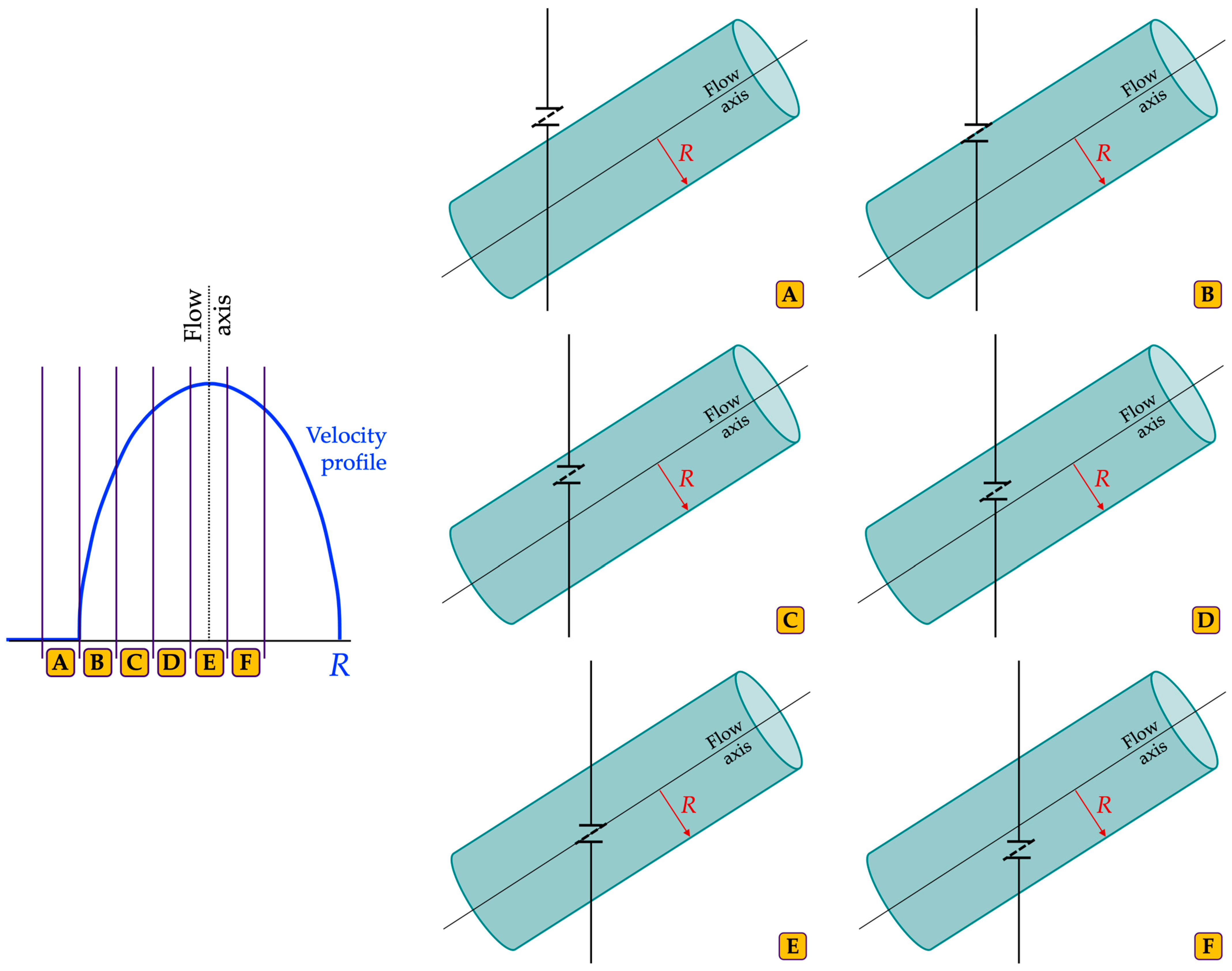
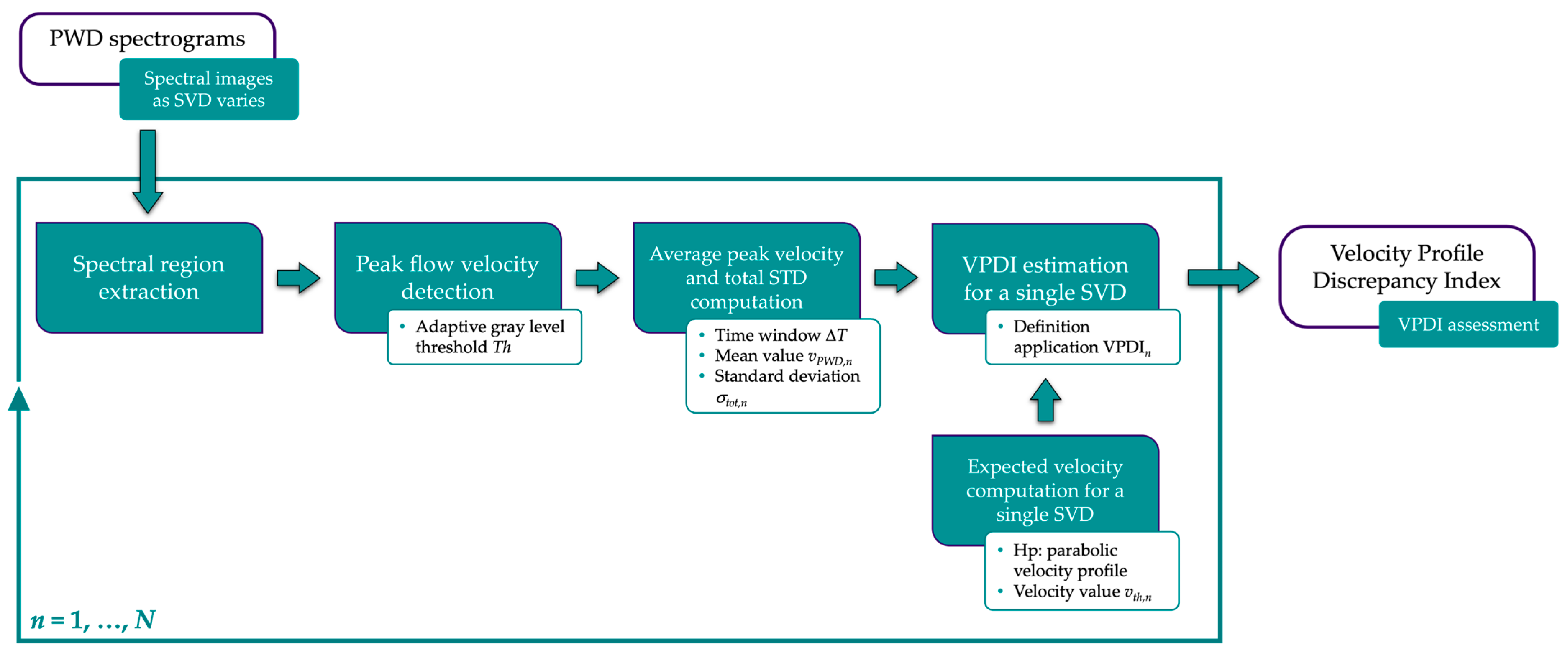
2.2.1. Velocity Profile Discrepancy Index
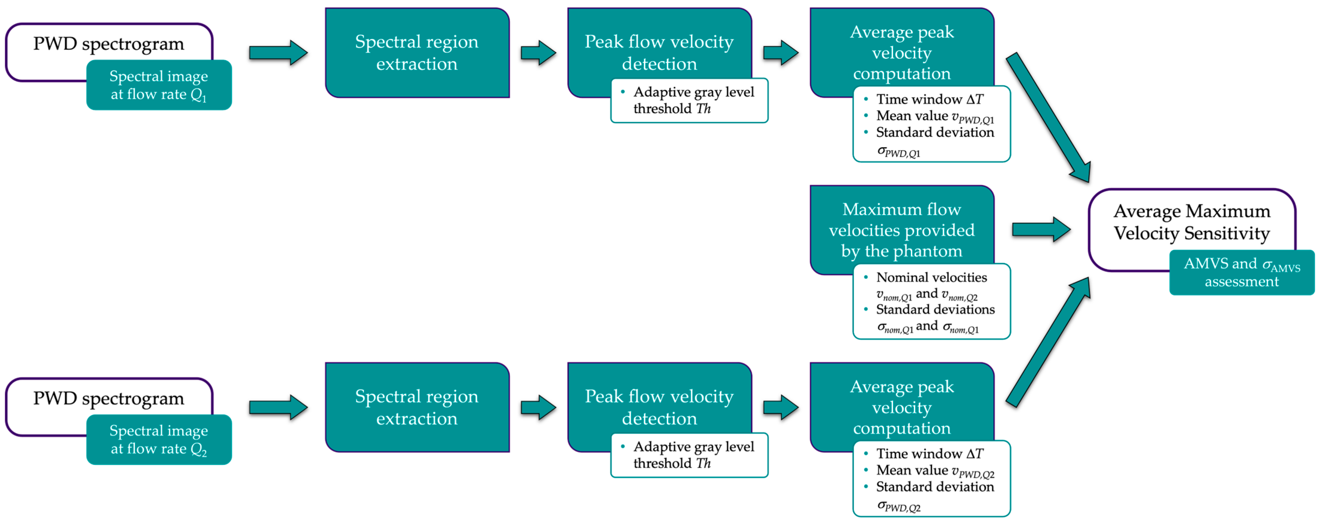
2.2.2. Average Maximum Velocity Sensitivity
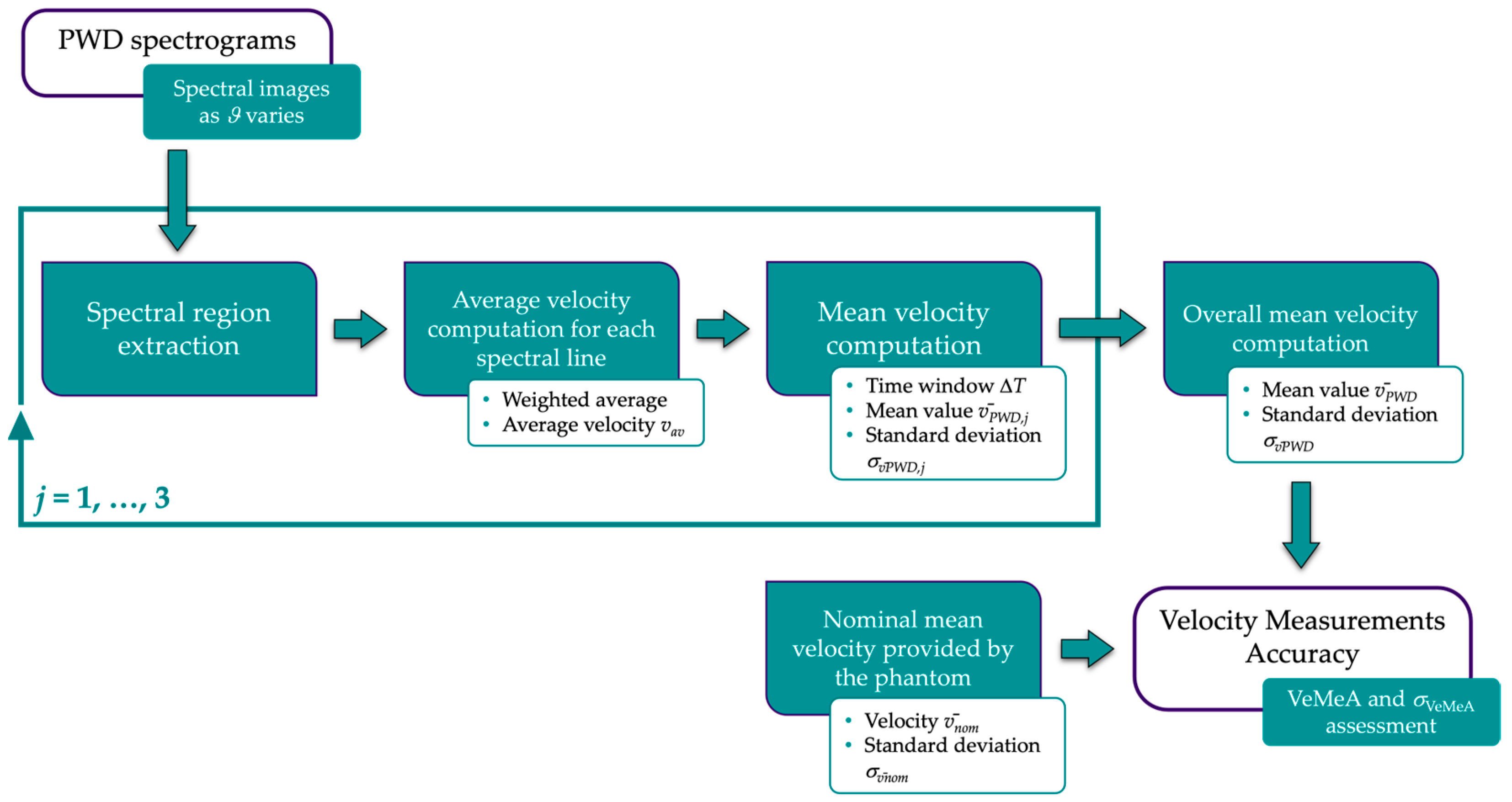
2.2.3. Velocity Measurements Accuracy
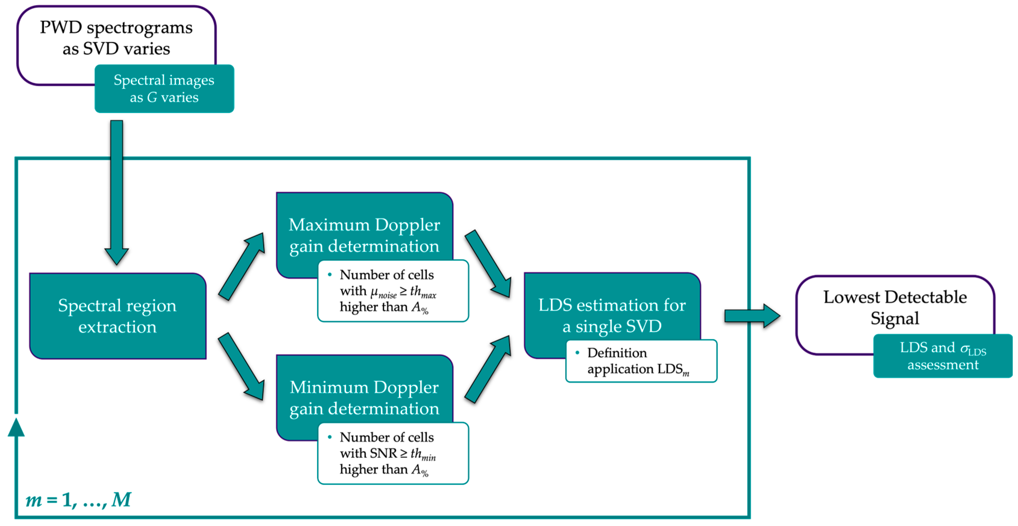
2.2.4. Lowest Detectable Signal
- For the first gain value, a region of interest, referred to as ROIn, is drawn at the top of each spectral image where the noise is expected to appear (Figure 6a). The size in pixels of the region is derived by considering a fixed window on the time axis and one on the velocity axis, ΔT and ΔV, respectively. ROIn is divided into cells of g × g pixels, and the average gray level μnoise,p is computed for each cell. Therefore, a further region of interest (ROIn2) is obtained, one for each spectral image, i.e., one for each Doppler gain setting. At this point, Gmax is determined as the lowest gain for which the number of cells in ROIn2 with μnoise,p ≥ thmax is greater than A% (expressed as a percentage of the total number of cells).
- For the second gain value, a further region of interest, referred to as ROIv, is drawn on the spectral images in addition to ROIn. As shown in Figure 6b, it maintains the same size (ΔT × ΔV) but is positioned to include pixels that on the velocity scale correspond to the nominal maximum velocity set on the reference device. The average gray level μNOISE of ROIn is computed as the noise level, whereas ROIv is divided into cells of g × g pixels, and the average gray level μsignal,p is computed for each cell, as in the previous case. Then, a Signal-to-Noise Ratio (SNR) matrix of elements g × g is derived, one for each spectral image, i.e., one for each Doppler gain setting:
2.3. Data Acquisition Protocol
2.4. Parameter Scaling
3. Measurement Uncertainty Analysis
- For both the VPDI and AMVS, simulations were performed by assuming a distribution of the adaptive threshold Thg, and the L spectral lines (corresponding to the time window ΔT) were randomized, at each iteration without repetition, among all those constituting the spectral image. The standard deviation of each output distribution σMCS was estimated and, for AMVS alone, this was combined with the repeatability STD σAMVS retrieved in Section 2.2.2;
- For VeMeA, only spectral line randomization was applied, and σMCS was combined with the repeatability standard deviation σVeMeA in Section 2.2.3;
- For LDS, an MCS was run for each SVD setting by assigning a distribution to the quantities in Equation (8), i.e., the attenuation coefficient of the phantom TMM, the sample volume depth, and the maximum as well as the minimum Doppler gain. The standard deviation σα was retrieved from the user’s guide of the reference device assuming a 95% confidence level, σz was derived from the sample volume depth resolution of 1 mm, while σGmax andσGmin were estimated from the Doppler gain step ΔG taken at the acquisition phase. Given the narrow bandwidth of the transmitted pulse, the uncertainty related to the Doppler frequency was considered negligible, and therefore no probability density function was assigned to fD. Finally, the STD of the parameter σLDS was estimated as the mean of the standard deviations of the M output distributions.
4. Results
5. Discussion and Conclusions
Author Contributions
Funding
Institutional Review Board Statement
Informed Consent Statement
Data Availability Statement
Acknowledgments
Conflicts of Interest
References
- Opieliński, K.J. Special issue on ultrasound technology in industry and medicine. Appl. Sci. 2023, 13, 1455. [Google Scholar] [CrossRef]
- Abhisheka, B.; Biswas, S.K.; Purkayastha, B.; Das, D.; Escargueil, A. Recent trend in medical imaging modalities and their applications in disease diagnosis: A review. Multimed. Tools Appl. 2024, 83, 43035–43070. [Google Scholar] [CrossRef]
- Wang, Y.; Chai, H.; Ye, R.; Li, J.; Liu, J.B.; Lin, C.; Peng, C. Point-of-care ultrasound: New concepts and future trends. Adv. Ultrasound Diagn. Ther. 2021, 5, 268–276. [Google Scholar] [CrossRef]
- Rix, A.; Lederle, W.; Theek, B.; Lammers, T.; Moonen, C.; Schmitz, G.; Kiessling, F. Advanced ultrasound technologies for diagnosis and therapy. J. Nucl. Med. 2018, 59, 740–746. [Google Scholar] [CrossRef] [PubMed]
- Gettle, L.M.; Revzin, M.V. Innovations in vascular ultrasound. Radiol. Clin. N. Am. 2020, 58, 653–669. [Google Scholar] [CrossRef] [PubMed]
- Zhang, R.; Wu, X.; Lou, Y.; Yan, F.-G.; Zhou, Z.; Wu, W.; Yuen, C. Channel training-aided target sensing for terahertz integrated sensing and massive MIMO communications. IEEE Internet Things J. 2024; early access. [Google Scholar] [CrossRef]
- Li, Y.; Wang, X.; Ding, Z. Multidimensional spectral super-resolution with prior knowledge with application to high mobility channel estimation. IEEE JSAC 2020, 38, 2836–2852. [Google Scholar] [CrossRef]
- Ferraz, S.; Coimbra, M.; Pedrosa, J. Assisted probe guidance in cardiac ultrasound: A review. Front. Cardiovasc. Med. 2023, 10, 1056055. [Google Scholar] [CrossRef] [PubMed]
- Fiorentino, M.C.; Villani, F.P.; Di Cosmo, M.; Frontoni, E.; Moccia, S. A review on deep-learning algorithms for fetal ultrasound-image analysis. Med. Imaging Anal. 2023, 83, 102629. [Google Scholar] [CrossRef] [PubMed]
- Aly, I.; Rizvi, A.; Roberts, W.; Khalid, S.; Kassem, M.W.; Salandy, S.; du Plessis, M.; Tubbs, R.S.; Loukas, M. Cardiac ultrasound: An anatomical and clinical review. Transl. Res. Anat. 2021, 22, 100083. [Google Scholar] [CrossRef]
- D’Andrea, A.; Conte, M.; Scarafile, R.; Riegler, L.; Cocchia, R.; Pezzullo, E.; Cavallaro, M.; Carbone, A.; Natale, F.; Russo, M.G.; et al. Transcranial Doppler ultrasound: Physical principles and principal applications in neurocritical care unit. J. Cardiovasc. Echogr. 2016, 26, 28–41. [Google Scholar] [CrossRef]
- Hamelmann, P.; Vullings, R.; Kolen, A.F.; Bergmans, J.W.M.; van Laar, J.O.E.H.; Tortoli, P.; Mischi, M. Doppler ultrasound technology for fetal heart rate monitoring: A review. IEEE Trans. Ultrason. Ferroelectr. Freq. Control 2020, 67, 226–238. [Google Scholar] [CrossRef] [PubMed]
- Levy, J.; Barrett, D.L.; Harris, N.; Jeong, J.J.; Yang, X.; Chen, S.C. High-frequency ultrasound in clinical dermatology: A review. Ultrasound J. 2021, 13, 24. [Google Scholar] [CrossRef] [PubMed]
- Demi, L.; Mento, F.; Di Sabatino, A.; Fiengo, A.; Sabatini, U.; Macioce, V.N.; Robol, M.; Tursi, F.; Sofia, C.; Di Cienzo, C.; et al. Lung ultrasound in COVID-19 and post-COVID-19 patients, an evidence-based approach. J. Ultrasound Med. 2022, 41, 2203–2215. [Google Scholar] [CrossRef] [PubMed]
- Barnett, S. Safety of diagnostic ultrasound. In Manual of Diagnostic Ultrasound, 2nd ed.; Buscarini, E., Lutz, H., Mirk, P., Eds.; WHO World Health Organization: Geneva, Switzerland, 2013; Volume 2, ISBN 978 92 4 154854 0. [Google Scholar]
- Hoskins, P.R. Principles of Doppler ultrasound. In Diagnostic Ultrasound Physics and Equipment, 3rd ed.; Hoskins, P.R., Martin, K., Thrush, A., Eds.; CRC Press: Boca Raton, FL, USA, 2019; pp. 143–158. [Google Scholar]
- McDicken, W.N.; Hoskins, P.R. Physics: Principles, Practice and Artefacts. In Clinical Doppler Ultrasound, 3rd ed.; Pozniak, M.A., Allan, P.L., Eds.; Churchill Livingstone: London, UK, 2013; pp. 1–25. [Google Scholar]
- Browne, J.E. A review of Doppler ultrasound quality assurance protocols and test devices. Phys. Med. 2014, 30, 742–751. [Google Scholar] [CrossRef] [PubMed]
- Balbis, S.; Meloni, T.; Tofani, S.; Zenone, F.; Nucera, D.; Guiot, C. Criteria and scheduling of quality control of B-mode and Doppler ultrasonography equipment. J. Clin. Ultrasound 2012, 40, 167–173. [Google Scholar] [CrossRef]
- ACR and AAPM Committees. ACR–AAPM Technical Standard for Diagnostic Medical Physics Performance Monitoring of Real Time Ultrasound Equipment—Revised. 2021. Available online: https://www.acr.org/-/media/ACR/Files/Practice-Parameters/us-equip.pdf?la=en (accessed on 14 September 2024).
- Lu, Z.F.; Hangiandreou, N.J.; Carson, P. Clinical ultrasonography physics: State of practice. In Clinical Imaging Physics: Current and Emerging Practice, 1st ed.; Samei, E., Pfeiffer, D.E., Eds.; Wiley Blackwell: Hoboken, NJ, USA, 2020; pp. 261–286. [Google Scholar]
- Lorentsson, R.; Hosseini, N.; Aurell, Y.; Collin, D.; Frösing, E.; Szaro, P.; Månsson, L.G.; Båth, M. Investigation of the impact of defective ultrasound transducers on clinical image quality in grayscale 2-D still images. Ultrasound Med. Biol. 2023, 49, 2126–2133. [Google Scholar] [CrossRef]
- Sipilä, O.; Mannila, V.; Vartiainen, E. Quality assurance in diagnostic ultrasound. Eur. J. Radiol. 2011, 80, 519–525. [Google Scholar] [CrossRef]
- Vachutka, J.; Dolezal, L.; Kollmann, C.; Klein, J. The effect of dead elements on the accuracy of Doppler ultrasound measurements. Ultrasound Imaging 2014, 36, 18–34. [Google Scholar] [CrossRef] [PubMed]
- Weigang, B.; Moore, G.W.; Gessert, J.; Phillips, W.H.; Schafer, M. The methods and effects of transducer degradation on image quality and the clinical efficacy of diagnostic sonography. J. Diagn. Med. Sonog. 2003, 19, 3–13. [Google Scholar] [CrossRef]
- Vitikainen, A.M.; Peltonen, J.I.; Vartiainen, E. Routine ultrasound quality assurance in a multi-unit radiology department: A retrospective evaluation of transducer failures. Ultrasound Med. Biol. 2017, 43, 1930–1937. [Google Scholar] [CrossRef]
- Dudley, N.J.; Woolley, D.J. A multicentre survey of the condition of ultrasound probes. Ultrasound 2016, 24, 190–197. [Google Scholar] [CrossRef] [PubMed]
- Hangiandreou, N.J.; Stekel, S.F.; Tradup, D.J.; Gorny, K.R.; King, D.M. Four-year experience with a clinical ultrasound quality control program. Ultrasound Med. Biol. 2011, 37, 1350–1357. [Google Scholar] [CrossRef] [PubMed]
- Mårtensson, M.; Olsson, M.; Segall, B.; Fraser, A.G.; Winter, R.; Brodin, L.-A. High incidence of defective ultrasound transducers in use in routine clinical practice. Eur. J. Echocardiogr. 2009, 10, 389–394. [Google Scholar] [CrossRef] [PubMed]
- Mårtensson, M.; Olsson, M.; Brodin, L.-Å. Ultrasound transducer function: Annual testing is not sufficient. Eur. J. Echocardiogr. 2010, 11, 801–805. [Google Scholar] [CrossRef] [PubMed]
- Cournane, S.; Fagan, A.J.; Browne, J.E. An audit of a hospital-based Doppler ultrasound quality control protocol using a commercial string Doppler phantom. Phys. Med. 2014, 30, 380–384. [Google Scholar] [CrossRef]
- Ambrogio, S.; Ansell, J.; Gabriel, E.; Aneju, G.; Newman, B.; Negoita, M.; Fedele, F.; Ramnarine, K.V. Pulsed wave Doppler measurements of maximum velocity: Dependence on sample volume size. Ultrasound Med. Biol. 2022, 48, 68–77. [Google Scholar] [CrossRef]
- Hangiandreou, J.; Carson, P.; Lu, Z.F. Clinical ultrasonography physics: Emerging practice. In Clinical Imaging Physics: Current and Emerging Practice, 1st ed.; Samei, E., Pfeiffer, D.E., Eds.; Wiley Blackwell: Hoboken, NJ, USA, 2020; pp. 287–302. [Google Scholar]
- IPEM Institute of Physics and Engineering in Medicine. Report 102: Quality Assurance of Ultrasound Imaging Systems, 1st ed.; IPEM Institute of Physics and Engineering in Medicine: York, UK, 2010. [Google Scholar]
- AIUM American Institute of Ultrasound in Medicine. Performance Criteria and Measurements for Doppler Ultrasound Devices, 2nd ed.; American Institute of Ultrasound in Medicine: Laurel, MD, USA, 2002. [Google Scholar]
- EFSUM. Technical Quality Evaluation of Diagnostic Ultrasound Systems—A Comprehensive Overview of Regulations and Developments. Available online: https://efsumb.org/wp-content/uploads/2023/07/ECB2nd_-TechnicalQuality_FULL.pdf (accessed on 14 September 2024).
- Thijssen, J.M.; van Wijk, M.C.; Cuypers, M.H. Performance testing of medical echo/Doppler equipment. Eur. J. Ultrasound 2002, 15, 151–164. [Google Scholar] [CrossRef]
- Fiori, G.; Pica, A.; Sciuto, S.A.; Marinozzi, F.; Bini, F.; Scorza, A. A comparative study on a novel quality assessment protocol based on image analysis methods for color Doppler ultrasound diagnostic systems. Sensors 2022, 22, 9868. [Google Scholar] [CrossRef]
- Fiori, G.; Schmid, M.; Galo, J.; Conforto, S.; Sciuto, S.A.; Scorza, A. Image quality assurance for B-mode diagnostic ultrasound: Kiviat-based protocol first application. In Proceedings of the 2024 IEEE International Workshop on Metrology for Industry 4.0 & IoT (MetroInd4.0 & IoT), Firenze, Italy, 29–31 May 2024. [Google Scholar] [CrossRef]
- Fiori, G.; Bocchetta, G.; Schmid, M.; Conforto, S.; Sciuto, S.A.; Scorza, A. Novel quality assessment protocol based on Kiviat diagram for pulsed wave Doppler diagnostic systems: First results. In Proceedings of the 26th IMEKO TC4 International Symposium and 24th International Workshop on ADC and DAC Modelling and Testing (IWADC), Pordenone, Italy, 20–21 September 2023. [Google Scholar] [CrossRef]
- Saary, M.J. Radar plots: A useful way for presenting multivariate health care data. J. Clin. Epidemiol. 2008, 61, 311–317. [Google Scholar] [CrossRef]
- Morales-Silva, D.M.; McPherson, C.S.; Pineda-Villavicencio, G.; Atchison, R. Using radar plots for performance benchmarking at patient and hospital levels using an Australian orthopaedics dataset. Health Inform. J. 2020, 26, 2119–2137. [Google Scholar] [CrossRef]
- Wang, R.C.; Edgar, T.F.; Baldea, M.; Nixon, M.; Wojsznis, W.; Dunia, R. Process fault detection using time-explicit Kiviat diagrams. AlChE J. 2015, 61, 4277–4293. [Google Scholar] [CrossRef]
- Fiori, G.; Scorza, A.; Schmid, M.; Galo, J.; Conforto, S.; Sciuto, S.A. A preliminary study on a novel approach to the assessment of the sample volume length and registration accuracy in PW Doppler quality control. In Proceedings of the 2022 IEEE International Symposium on Medical Measurements and Applications (MeMeA), Messina, Italy, 22–24 June 2022. [Google Scholar] [CrossRef]
- Fiori, G.; Bocchetta, G.; Conforto, S.; Sciuto, S.A.; Scorza, A. Sample volume length and registration accuracy assessment in quality controls of PW Doppler diagnostic systems: A comparative study. Acta IMEKO 2023, 12, 2. [Google Scholar] [CrossRef]
- Fiori, G.; Fuiano, F.; Scorza, A.; Schmid, M.; Galo, J.; Conforto, S.; Sciuto, S.A. A novel sensitivity index from the flow velocity variation in quality control for PW Doppler: A preliminary study. In Proceedings of the 2021 IEEE International Symposium on Medical Measurements and Applications (MeMeA), Lausanne, Switzerland, 23–25 June 2021. [Google Scholar] [CrossRef]
- Fiori, G.; Fuiano, F.; Scorza, A.; Galo, J.; Conforto, S.; Sciuto, S.A. A preliminary study on an image analysis based method for lowest detectable signal measurements in pulsed wave Doppler ultrasounds. Acta IMEKO 2021, 10, 126–132. [Google Scholar] [CrossRef]
- Fiori, G.; Fuiano, F.; Scorza, A.; Galo, J.; Conforto, S.; Sciuto, S.A. Lowest detectable signal in medical PW Doppler quality control by means of a commercial flow phantom: A case study. In Proceedings of the 24th IMEKO TC4 International Symposium and 22nd International Workshop on ADC and DAC Modelling and Testing (IWADC), Palermo, Italy, 14–16 September 2020; Available online: https://www.imeko.org/publications/tc4-2020/IMEKO-TC4-2020-63.pdf (accessed on 14 September 2024).
- Fiori, G.; Fuiano, F.; Scorza, A.; Schmid, M.; Conforto, S.; Sciuto, S.A. Doppler flow phantom failure detection by combining empirical mode decomposition and independent component analysis with short time Fourier transform. Acta IMEKO 2021, 10, 185–193. [Google Scholar] [CrossRef]
- Sun Nuclear Corporation. Doppler 403™ & Mini-Doppler 1430™ Flow Phantoms. Available online: https://www.sunnuclear.com/uploads/documents/datasheets/Diagnostic/DopplerFlow_Phantoms_113020.pdf (accessed on 14 September 2024).
- Sun Nuclear Corporation. Doppler Ultrasound Phantoms. Available online: https://www.sunnuclear.com/products/doppler-ultrasound-phantoms (accessed on 14 September 2024).
- Thrush, A. Spectral Doppler ultrasound. In Diagnostic Ultrasound Physics and Equipment, 3rd ed.; Hoskins, P.R., Martin, K., Thrush, A., Eds.; CRC Press: Boca Raton, FL, USA, 2019; pp. 171–189. [Google Scholar]
- IEC International Electrotechnical Commission. IEC TS 61895:1999-10: Ultrasonics—Pulsed Doppler Diagnostic Systems—Test Procedures to Determine Performance, 1st ed.; International Electrotechnical Committee: Geneva, Switzerland, 1999. [Google Scholar]
- Grant, E.G.; Benson, C.B.; Moneta, G.L.; Alexandrov, A.V.; Baker, J.D.; Bluth, E.I.; Carroll, B.A.; Eliasziw, M.; Gocke, J.; Hertzberg, B.S.; et al. Carotid artery stenosis: Gray-scale and Doppler US diagnosis--Society of Radiologists in Ultrasound Consensus Conference. Radiology 2003, 229, 340–346. [Google Scholar] [CrossRef]
- Anavekar, N.S.; Oh, J.K. Doppler echocardiography: A contemporary review. J Cardiol. 2009, 54, 347–358. [Google Scholar] [CrossRef]
- Campbell, K.A.; Kupinski, A.M.; Miele, F.R.; Silva, P.F.; Zierler, R.E. Changes in internal carotid artery Doppler velocity measurements with different angles of insonation: A pilot study. J. Ultrasound Med. 2021, 40, 1937–1948. [Google Scholar] [CrossRef]
- Park, M.Y.; Jung, S.E.; Byun, J.Y.; Kim, J.H.; Joo, G.E. Effect of beam-flow angle on velocity measurements in modern Doppler ultrasound systems. AJR Am. J. Roentgenol. 2012, 198, 1139–1143. [Google Scholar] [CrossRef]
- Marinozzi, F.; Bini, F.; D’Orazio, A.; Scorza, A. Performance tests of sonographic instruments for the measure of flow speed. In Proceedings of the 2008 IEEE International Workshop on Imaging Systems and Techniques, Chania, Greece, 10–12 September 2008. [Google Scholar] [CrossRef]
- Boote, E.J.; Zagzebski, J.A. Performance tests of Doppler ultrasound equipment with a tissue and blood-mimicking phantom. J. Ultrasound Med. 1988, 7, 137–147. [Google Scholar] [CrossRef]
- ISO International Organization for Standardization and IEC International Electrotechnical Commission. ISO/IEC Guide 99:2007: International Vocabulary of Metrology—Basic and General Concepts and Associated Terms (VIM), 1st ed.; International Organization for Standardization Technical Management Board: Geneva, Switzerland, 2007. [Google Scholar]
- ISO International Organization for Standardization and IEC International Electrotechnical Commission. ISO/IEC Guide 98-3/Suppl.1:2008: Uncertainty of Measurement—Part 3: Guide to the Expression of Uncertainty in Measurement (GUM:1995)—Supplement 1: Propagation of Distributions Using a Monte Carlo Method, 1st ed.; International Organization for Standardization Technical Management Board: Geneva, Switzerland, 2008. [Google Scholar]
- Papadopoulos, C.E.; Yeung, H. Uncertainty estimation and Monte Carlo simulation method. Flow Meas. Instrum. 2001, 12, 291–298. [Google Scholar] [CrossRef]
- Motra, H.B.; Hildebrand, J.; Wuttke, F. The Monte Carlo method for evaluating measurement uncertainty: Application for determining the properties of materials. Probabilistic Eng. Mech. 2016, 45, 220–228. [Google Scholar] [CrossRef]
- Fiori, G.; Fuiano, F.; Schmid, M.; Conforto, S.; Sciuto, S.A.; Scorza, A. A comparative study on depth of penetration measurements in diagnostic ultrasounds through the adaptive SNR threshold method. IEEE Trans. Instrum. Meas. 2023, 72, 4003108. [Google Scholar] [CrossRef]
- Taylor, J.R. An Introduction to Error Analysis: The Study of Uncertainties in Physical Measurements, 2nd ed.; University Science Books: Sausalito, CA, USA, 1996; pp. 245–260. [Google Scholar]
- Yiu, B.Y.S.; Yu, A.C.H. Spiral flow phantom for ultrasound flow imaging experimentation. IEEE Trans. Ultrason. Ferroelectr. Freq. Control 2017, 64, 1840–1848. [Google Scholar] [CrossRef] [PubMed]
- Russo, D.; Ricci, S. Electronic flow emulator for the test of ultrasound Doppler sensors. IEEE Trans. Ind. Electron. 2022, 69, 6341–6349. [Google Scholar] [CrossRef]
- Lee, H.K.; Greenleaf, J.F.; Urban, M.W. A new plane wave compounding scheme using phase compensation for motion detection. IEEE Trans. Ultrason. Ferroelectr. Freq. Control 2022, 69, 702–710. [Google Scholar] [CrossRef]
- Ramalli, A.; Boni, E.; Roux, E.; Liebgott, H.; Tortoli, P. Design, implementation, and medical applications of 2-D ultrasound sparse arrays. IEEE Trans. Ultrason. Ferroelectr. Freq. Control 2022, 69, 2739–2755. [Google Scholar] [CrossRef]


| Setting | Pre-Set | UDS1 | UDS2 | UDS3 | UDS4 | UDS5 |
|---|---|---|---|---|---|---|
| Field of view (cm) | A and B | 7 | 7 | 7 | 7 | 7 |
| Doppler frequency (MHz) | A and B | 5.0 | 5.0 | 5.0 | 5.0 | 5.5 |
| Wall filter | A | medium | high | medium | low | low |
| B | minimum | minimum | minimum | minimum | minimum | |
| Compression | A | medium | low | medium | medium | low |
| B | minimum | minimum | minimum | minimum | minimum | |
| Power | A | maximum | maximum | high | high | high |
| B | maximum | maximum | maximum | maximum | maximum | |
| Doppler baseline | A and B | minimum | minimum | minimum | minimum | minimum |
| Spectrogram resolution (px × px) | A and B | 960 × 1280 | 478 × 900 | 455 × 1210 | 345 × 1690 | 480 × 1365 |
| Spectrogram duration (s) | A and B | 9.5 | 8 | 12 | ~12 | ~11 |
| Feature | Specification |
|---|---|
| Phantom model | Doppler 403TM flow phantom (Sun Nuclear corporation, Middleton, WI, USA) |
| Horizontal vessel | 5.0 ± 0.2 mm inner diameter at 2 cm depth |
| Diagonal vessel | 5.0 ± 0.2 mm inner diameter at 40° from 2 to 16 cm deep |
| Attenuation coefficient | 0.70 ± 0.05 dB·cm−1·MHz−1 |
| Scanning surface | patented composite film |
| TMM | patented High Equivalency GelTM |
| TMM sound speed | 1540 ± 10 m·s−1 |
| BMF sound speed | 1550 ± 10 m·s−1 |
| Flow range | (1.7–12.5) ± 0.4 mL·s−1 |
| Flow rate | customizable, constant, and pulsatile |
| Dimensions (case) | 28.0 × 30.5 × 22.0 cm |
| Feature | Symbol | Value |
|---|---|---|
| Adaptive threshold | Th | 10% of the maximum gray level displayed |
| Time window | ΔT | 7 s |
| Number of spectral lines | L | varies with the resolution and duration of the PWD spectrogram |
| Minimum SVL increment | Δl | 1 mm |
| Number of SV depths | N | 7 |
| Feature | Symbol | Value |
|---|---|---|
| Adaptive threshold | Th | 10% of the maximum gray level displayed |
| Time window | ΔT | 7 s |
| Number of spectral lines | L | varies with the resolution and duration of the PWD spectrogram |
| Feature | Symbol | Value |
|---|---|---|
| Time window | ΔT | 7 s |
| Number of spectral lines | L | varies with the resolution and duration of the PWD spectrogram |
| Feature | Symbol | Value |
|---|---|---|
| Time window | ΔT | 7 s |
| Velocity window | ΔV | 15 cm·s−1 |
| Cell size | g × g | 6 × 6 px |
| Threshold for Gmax determination | thmax | 3 |
| Threshold for Gmin determination | thmin | 2 |
| Percentage of the total number of cells | A% | 1% |
| Number of SV depths | M | 5 |
| Parameter | Flow Rate (mL·s−1) | Average Velocity (cm·s−1) | Maximum Velocity (cm·s−1) |
|---|---|---|---|
| VPDI | 7.0 | 35.7 | 71.3 |
| AMVS | 5.5 and 7.0 | 28.0 and 35.7 | 56.0 and 71.3 |
| VeMeA | 7.0 | 35.7 | 71.3 |
| LDS | 2.0 | 10.2 | 20.4 |
| Setting | Parameter | UDS1 | UDS2 | UDS3 | UDS4 | UDS5 |
|---|---|---|---|---|---|---|
| Sample volume length (mm) | VPDI | 1.0 | 1.0 | 1.0 | 1.0 | 1.0 |
| AMVS | 1.0 | 1.0 | 1.0 | 1.0 | 1.0 | |
| VeMeA | 1.0 | 1.0 | 1.0 | 1.0 | 1.0 | |
| LDS | 1.5 | 2.0 | 1.5 | 1.5 | 1.5 | |
| Sample volume depth (mm) | VPDI | 35 to 41; 1 mm spaced | 35 to 41; 1 mm spaced | 35 to 41; 1 mm spaced | 35 to 41; 1 mm spaced | 35 to 41; 1 mm spaced |
| AMVS | 40 | 40 | 40 | 40 | 40 | |
| VeMeA | 40 | 40 | 40 | 40 | 40 | |
| LDS | 42 to 50; 2 mm spaced | 38 to 46; 2 mm spaced | 48 to 56; 2 mm spaced | 62 to 70; 2 mm spaced | 42 to 50; 2 mm spaced | |
| Correction angle (°) | VPDI | 50 | 50 | 50 | 50 | 50 |
| AMVS | 50 | 50 | 50 | 50 | 50 | |
| VeMeA | 50 ± 1 | 50 ± 1 | 50 ± 1 | 50 ± 2 | 50 ± 1 | |
| LDS | 50 | 50 | 50 | 50 | 50 |
| Ultrasound System | Doppler Gain | ||
|---|---|---|---|
| Range | Gain Step ΔG | Measurement Unit | |
| UDS1 | from 0 to 50 | 2 | dB |
| UDS2 | from 0 to 85 | 5 | dB |
| UDS3 | from 0 to 100 | 2 | a.u. (1) |
| UDS4 | from 0 to 100 | 4 | % |
| UDS5 | from 0 to 100 | 2 | a.u. (1) |
| Test Parameter | Acronym | Expected Value |
|---|---|---|
| Velocity profile discrepancy index | VPDI | 0 |
| Average maximum velocity sensitivity | AMVS | 1 |
| Velocity measurements accuracy | VeMeA | 0 |
| Lowest detectable signal | LDS | Bmax (1) |
| VPDI and AMVS | Symbol | Mean ± STD | |
|---|---|---|---|
| Adaptive gray level threshold | Thg ± σThg | uniform | (10% ± 1%) of glmax (1) |
| Spectral line randomization | - | - | - |
| VeMeA | |||
| Spectral line randomization | - | - | - |
| LDS | |||
| TMM attenuation (dB·cm−1·MHz−1) | α ± σα | normal | 0.700 ± 0.025 |
| Sample volume depth (mm) | z ± σz | uniform | z ± 0.3 |
| Maximum Doppler gain | Gmax ± σGmax | uniform | Gmax ± ΔG/2√3 |
| Minimum Doppler gain | Gmin ± σGmin | uniform | Gmin ± ΔG/2√3 |
| Ultrasound System | Pre-Set | VPDI | AMVS | VeMeA | LDS (dB) |
|---|---|---|---|---|---|
| UDS1 | A | 0.35 ± 0.03 | 1.2 ± 0.3 | 0.90 ± 0.09 | 47.4 ± 1.4 |
| B | 1.00 ± 0.24 | 1.3 ± 0.4 | 0.96 ± 0.09 | 47.0 ± 1.4 | |
| UDS2 | A | 0.15 ± 0.09 | 1.0 ± 0.3 | 0.87 ± 0.09 | 53.4 ± 2.3 |
| B | 0.08 ± 0.01 | 0.9 ± 0.3 | 0.96 ± 0.09 | 50.4 ± 2.3 | |
| UDS3 | A | 0.47 ± 0.04 | 1.2 ± 0.3 | 0.88 ± 0.09 | 49 ± 5 |
| B | 0.64 ± 0.05 | 1.2 ± 0.4 | 0.82 ± 0.08 | 53 ± 5 | |
| UDS4 | A | 2.01 ± 0.23 | 1.0 ± 0.3 | 0.95 ± 0.09 | 51.7 ± 2.3 |
| B | 0.38 ± 0.02 | 1.0 ± 0.3 | 0.94 ± 0.09 | N.A. (1) | |
| UDS5 | A | 2.67 ± 0.17 | 1.1 ± 0.3 | 0.75 ± 0.08 | 49 ± 4 |
| B | 0.72 ± 0.07 | 1.2 ± 0.3 | 0.81 ± 0.08 | 50 ± 5 |
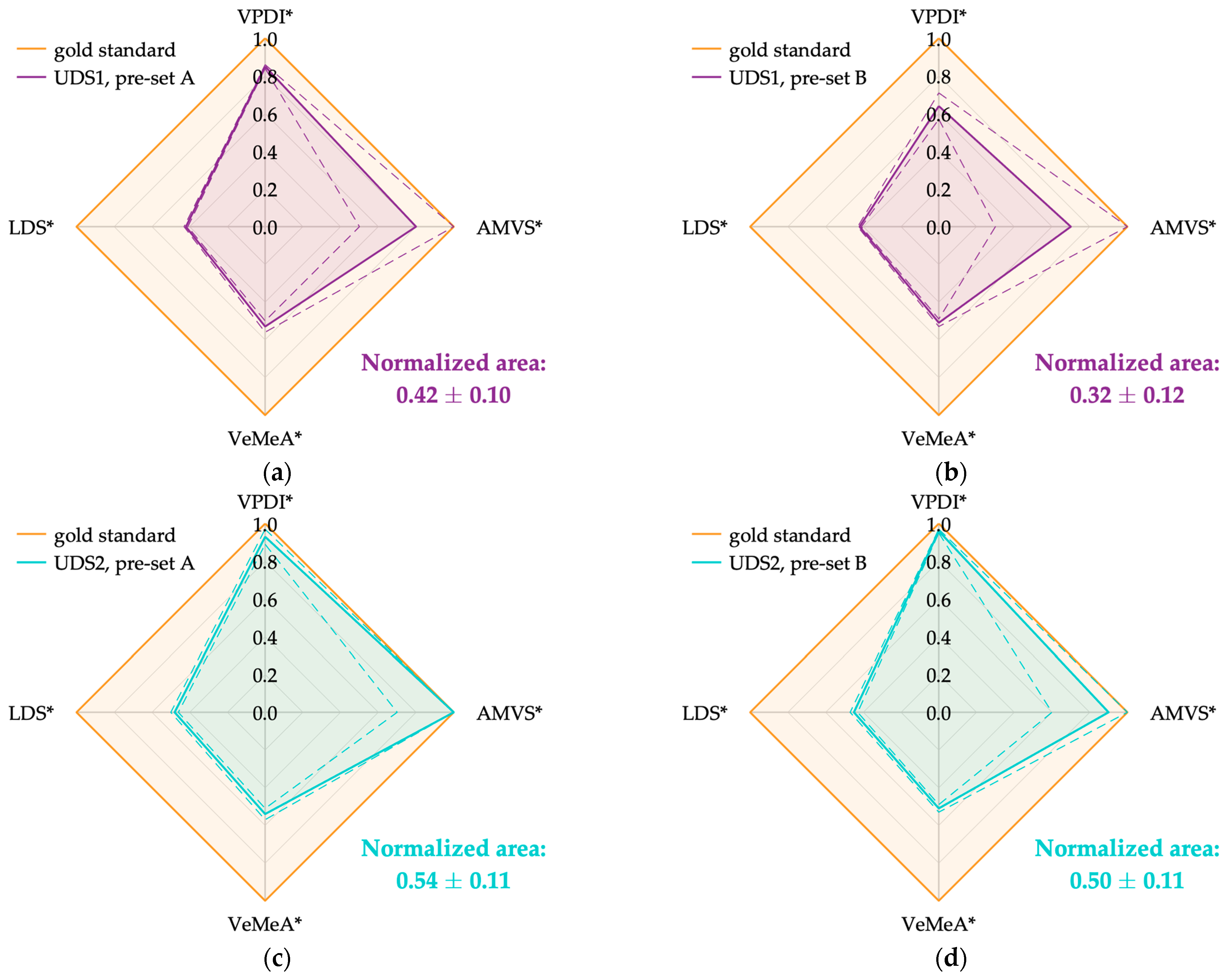
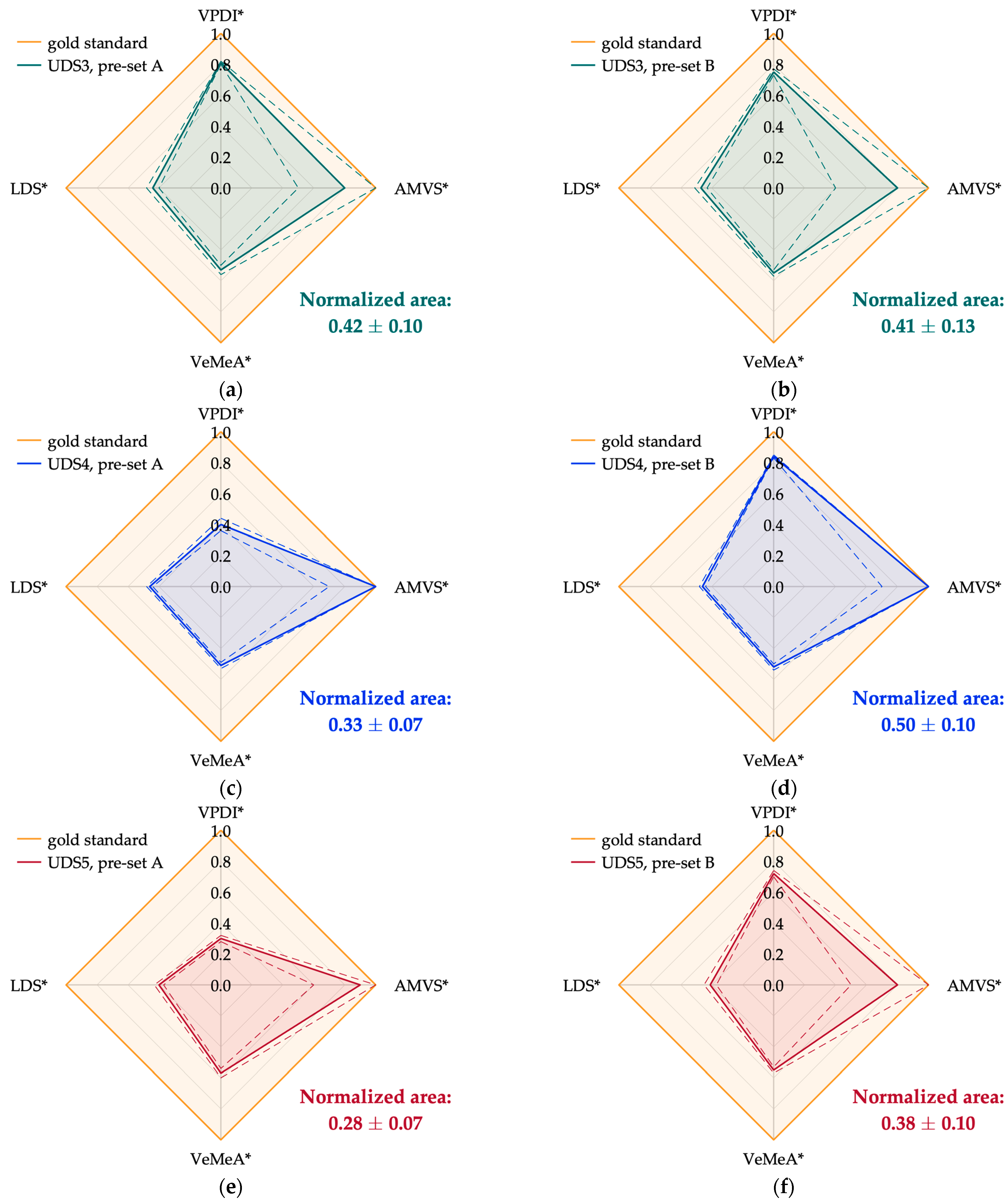
| Ultrasound System | Pre-Set | VPDI* | AMVS* | VeMeA* | LDS* | Normalized Area |
|---|---|---|---|---|---|---|
| UDS1 | A | 0.85 ± 0.01 | 0.8 ± 0.3 | 0.53 ± 0.03 | 0.42 ± 0.01 | 0.42 ± 0.10 |
| B | 0.64 ± 0.07 | 0.7 ± 0.4 | 0.51 ± 0.02 | 0.42 ± 0.01 | 0.32 ± 0.12 | |
| UDS2 | A | 0.93 ± 0.04 | 1.0 ± 0.3 | 0.54 ± 0.03 | 0.48 ± 0.02 | 0.54 ± 0.11 |
| B | 0.96 ± 0.01 | 0.9 ± 0.3 | 0.51 ± 0.02 | 0.45 ± 0.02 | 0.50 ± 0.11 | |
| UDS3 | A | 0.81 ± 0.01 | 0.8 ± 0.3 | 0.53 ± 0.03 | 0.44 ± 0.04 | 0.42 ± 0.10 |
| B | 0.75 ± 0.02 | 0.8 ± 0.4 | 0.55 ± 0.02 | 0.47 ± 0.04 | 0.41 ± 0.13 | |
| UDS4 | A | 0.40 ± 0.04 | 1.0 ± 0.3 | 0.51 ± 0.02 | 0.46 ± 0.02 | 0.33 ± 0.07 |
| B | 0.84 ± 0.01 | 1.0 ± 0.3 | 0.52 ± 0.02 | N.A. (1) | 0.50 ± 0.10 (2) | |
| UDS5 | A | 0.30 ± 0.02 | 0.9 ± 0.3 | 0.57 ± 0.03 | 0.40 ± 0.03 | 0.28 ± 0.07 |
| B | 0.72 ± 0.02 | 0.8 ± 0.3 | 0.55 ± 0.02 | 0.41 ± 0.04 | 0.38 ± 0.10 |
Disclaimer/Publisher’s Note: The statements, opinions and data contained in all publications are solely those of the individual author(s) and contributor(s) and not of MDPI and/or the editor(s). MDPI and/or the editor(s) disclaim responsibility for any injury to people or property resulting from any ideas, methods, instructions or products referred to in the content. |
© 2024 by the authors. Licensee MDPI, Basel, Switzerland. This article is an open access article distributed under the terms and conditions of the Creative Commons Attribution (CC BY) license (https://creativecommons.org/licenses/by/4.0/).
Share and Cite
Fiori, G.; Scorza, A.; Schmid, M.; Conforto, S.; Sciuto, S.A. Comparative Approach to Performance Estimation of Pulsed Wave Doppler Equipment Based on Kiviat Diagram. Sensors 2024, 24, 6491. https://doi.org/10.3390/s24196491
Fiori G, Scorza A, Schmid M, Conforto S, Sciuto SA. Comparative Approach to Performance Estimation of Pulsed Wave Doppler Equipment Based on Kiviat Diagram. Sensors. 2024; 24(19):6491. https://doi.org/10.3390/s24196491
Chicago/Turabian StyleFiori, Giorgia, Andrea Scorza, Maurizio Schmid, Silvia Conforto, and Salvatore Andrea Sciuto. 2024. "Comparative Approach to Performance Estimation of Pulsed Wave Doppler Equipment Based on Kiviat Diagram" Sensors 24, no. 19: 6491. https://doi.org/10.3390/s24196491