Abstract
SLAM (Simultaneous Localization and Mapping) based on 3D LiDAR (Laser Detection and Ranging) is an expanding field of research with numerous applications in the areas of autonomous driving, mobile robotics, and UAVs (Unmanned Aerial Vehicles). However, in most real-world scenarios, dynamic objects can negatively impact the accuracy and robustness of SLAM. In recent years, the challenge of achieving optimal SLAM performance in dynamic environments has led to the emergence of various research efforts, but there has been relatively little relevant review. This work delves into the development process and current state of SLAM based on 3D LiDAR in dynamic environments. After analyzing the necessity and importance of filtering dynamic objects in SLAM, this paper is developed from two dimensions. At the solution-oriented level, mainstream methods of filtering dynamic targets in 3D point cloud are introduced in detail, such as the ray-tracing-based approach, the visibility-based approach, the segmentation-based approach, and others. Then, at the problem-oriented level, this paper classifies dynamic objects and summarizes the corresponding processing strategies for different categories in the SLAM framework, such as online real-time filtering, post-processing after the mapping, and Long-term SLAM. Finally, the development trends and research directions of dynamic object filtering in SLAM based on 3D LiDAR are discussed and predicted.
1. Introduction
SLAM (Simultaneous Localization and Mapping) is a cutting-edge technology that depends on specific environmental sensors to achieve self-localization in a given environment while simultaneously creating a model of the surrounding scene. This innovative technology has gained widespread recognition and adoption across several domains, including autonomous robots [1] and various intelligent fields. A typical SLAM system consists of a front-end module and a back-end module [2,3]. The front-end module collects data such as LiDAR (Laser Detection and Ranging) point clouds and camera images from sensors and finds the transformation between consecutive data frames, and the back-end module corrects the front-end estimation drifts by performing the loop closures [4].
SLAM based on 3D LiDAR is a technique that uses 3D laser scanners to perform simultaneous localization and mapping of an environment. 3D LiDAR is an active sensor that emits laser beams in multiple directions and measures the travel time and the phase difference of the reflected beams to create a 3D point cloud of the environment. The point cloud represents the spatial layout of the environment, which can be used to build a map and localize the robot within it. As research in the field of 3D LiDAR continues to advance [5,6], the exploration of SLAM technology based on this has gained significant momentum across various domains [7,8,9,10,11,12,13,14,15,16,17]. Consequently, numerous remarkable algorithms have been developed [18,19,20,21,22,23,24,25,26], with the most widely adopted ones being LOAM(LiDAR Odometry and Mapping) [20], and its various variants [2,21,22]; LIO (LiDAR-Inertial Odometry) [23,24,27,28]; and R3LIVE [25,26].
Notably, mainstream SLAM algorithms and point cloud alignment methods [29,30] are primarily developed under the premise of a static environment, while inadequately taking into account dynamic objects in the spatial realm. However, in real-world applications, an abundance of dynamic objects exists, such as pedestrians, vehicles, cyclists, temporary facilities or structures, and the like. In the street view shown in Figure 1, several common dynamic objects have been framed.
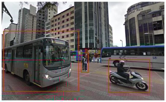
Figure 1.
Common Dynamic Objects in the street view.
The presence of dynamic objects can make it inevitable that the scan data from 3D LiDAR includes representations of them [31,32,33,34,35], thereby significantly impeding the effectiveness of SLAM algorithm implementation, with three main detrimental effects as shown below:
- At the front-end level, the accuracy of point cloud alignment can be affected by the presence of dynamic objects, and even the robustness of SLAM alignment algorithms may be severely compromised if there is an excessive number of dynamic point clouds.
- At the mapping level, various approaches have been proposed to model 3D environments [36,37] or sub-sampled representations [38,39]. However, full resolution 3D point clouds form a basis for extracting useful information from the map [32]. The presence of a significant number of dynamic point clouds in the 3D point cloud can result in a plethora of ghost-trail effects [32,40], which may obscure or overlap with the static features in the scene. This can severely hamper the effectiveness of the mapping.
- At the map-based localization level, the presence of numerous dynamic point clouds in the priori map can result in significant deviations between the priori map and current observations, and even act as obstacles that can interfere with the localization performance [41,42,43]. These effects can also hurt long-term map maintenance.
As previously discussed, the presence of dynamic objects can substantially compromise the accuracy and robustness of SLAM in various real-world scenarios, such as navigating dense crowds [44] and urban autonomous driving [45], resulting in degraded performance and potential safety hazards. It can be seen that detecting and filtering dynamic objects is a critical problem to be addressed in SLAM. This work aims to summarize how SLAM based on 3D LiDAR can effectively filter out dynamic objects in changing environments. The entire pipeline is demonstrated in Figure 2 and the main contributions are summarized as follows:
- Regarding the research of filtering dynamic objects in SLAM based on 3D LiDAR, this work proposes a comprehensive examination from two dimensions: the solution-oriented level and the problem-oriented level. The former concentrates on exploring the diverse underlying principles behind specific methods for detecting dynamic targets in 3D point cloud. The latter, on the other hand, focuses on the application of dynamic point cloud filtering techniques in downstream tasks, investigating the efficient removal of various dynamic objects in real-world scenarios within the overarching framework of SLAM. It explores the adoption of processing strategies tailored to match the dynamic degree of these dynamic objects, enabling rapid and effective filtering. Despite their distinct natures, these two dimensions are interconnected, as the principles governing the methods used in studies with different processing strategies may coincide. Similarly, methods based on different principles can find application within the same processing strategy.
- According to the different principles of detecting dynamic targets in a 3D point cloud, the dynamic point cloud filtering methods fall under different classifications, such as the ray-tracing-based approach, the visibility-based approach, the segmentation-based approach and others, and the main idea and problems of various methods are summarized.
- The classification of dynamic objects in the real-world according to their degree of dynamics and their different processing strategies, from online real-time filtering to post-processing after the mapping to Long-term SLAM for different categories of dynamic objects in the SLAM framework based on 3D LiDAR are presented, to help readers effectively choose a more appropriate solution for their specific applications.
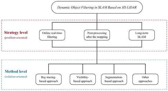
Figure 2.
The pipeline of this paper. We present a summary of filtering dynamic objects in SLAM based on 3D LiDAR from two dimensions: the Method level and the Strategy level. The Method level is solution-oriented, we categorize the specific methods for filtering dynamic targets in a 3D point cloud into the ray-tracing-based approach, the visibility-based approach, the segmentation-based approach, and others, each based on distinct detection principles. The Strategy level is problem-oriented, and in conjunction with the SLAM framework based on 3D LiDAR, we propose three diverse processing strategies tailored to objects exhibiting different degrees of dynamics: online real-time filtering, post-processing after the mapping, and Long-term SLAM.
This paper presents a comprehensive overview of dynamic object filtering techniques in SLAM based on 3D LiDAR, divided into four parts. The first section emphasizes the necessity and importance of dynamic object filtering in SLAM. Subsequently, the paper is structured around the integration of dual dimensions. First, at the solution-oriented level, Section 2 elucidates a selection of mainstream methods based on their principles, along with the various research carried out using each method. Then, at the problem-oriented level, in Section 3 dynamic objects are classified according to their degree of dynamics, the processing strategies for different categories of dynamic objects in the SLAM framework are summarized, and the advantages and disadvantages of representative algorithms from different methods are analyzed and compared. Finally, Section 4 offers a summary of the entire paper and an outlook on future research directions. Table 1 provides a list of abbreviations used in this paper.

Table 1.
Abbreviations for terms.
2. Dynamic Target Filtering Methods in the 3D Point Cloud
Section 1 of this work highlights how the presence of dynamic objects in realistic scenes can significantly compromise the robustness of SLAM. Unfortunately, many SLAM algorithms based on 3D LiDAR rely on the assumption of static backgrounds and thus are ill-equipped to handle such complex dynamic scenes [46]. Consequently, the point cloud belonging to the dynamic objects must be filtered out to obtain a clean 3D model of the whole scene, as shown in Figure 3. This research falls within the domain of change detection [47], and in this section a comprehensive summary of the universal dynamic point cloud filtering methods based on different principles, and their associated research work will be provided, approaching the topic from the solution-oriented dimension.
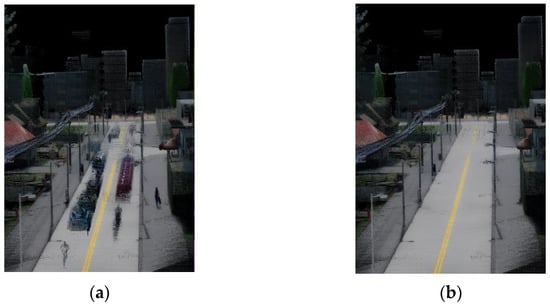
Figure 3.
(a) The original unprocessed point cloud; (b) The point cloud after filtering out dynamic target points.
2.1. Ray-Tracing-Based Approach
This type of method is based on ray tracing [48]. The entire scene space obtained by scanning is initially divided into occupancy voxel grids [49] (or octree grids [50]). The principle of this approach is that the dynamic point cloud only appears in a few scans, so the grid it belongs to is only briefly hit by the laser ray, whereas the laser’s light path passes through it in most cases. The marker is stored in each grid, representing the number of times it is hit or the probability of being hit by laser rays. By traversing all the grids in the point cloud, the grids with marker values below a certain threshold are identified as dynamic grids and all points that fall within them are removed. The illustration in Figure 4 shows the principle of this method. In the last decade, several studies have utilized this approach and obtained promising results.
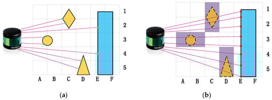
Figure 4.
The gray raster marks the 2D voxel boundaries. Magenta lines mark the scanner lines of sight. The blue shape represents a static object, while the yellow shapes represent dynamic objects. Green and red dots represent the measured points taken from two different scans: scan-I and scan-II. (a) The dynamic objects appear briefly in scan-I and are hit by lasers. (b) The dynamic objects disappear in scan-II and are passed through by lasers, and the grids A3, B3, C1, C2, D4, and D5 (the purple grids) where they are located are identified as dynamic grids, allowing filtering out of the point cloud within them.
In [51], Azim and Aycard employed the ray-tracing-based approach for dynamic object filtering in SLAM based on 3D LiDAR. Their proposed method involved identifying dynamic voxels initially by comparing the grid’s status of being marked as free or not free between the before and after scans. Then, by using an algorithm of clustering and by setting a threshold they verified whether these dynamic voxels represented dynamic objects. The study also categorized each cluster by calculating the ratio of the length, width, and height of the enclosing boxes, which further refined the accuracy of dynamic object detection by tracking the motion characteristics of the different object categories. However, the method’s robustness is limited in chaotic dynamic environments, and Azim and Aycard only provided a qualitative analysis of their approach.
Underwood et al. proposed an early and efficient 3D dynamic detection algorithm based on ray-tracing points in a spherical coordinate system [52]. However, the method has a limitation in that it did not construct a global occupancy grid and could only compare two scans at a time. This means that for a map consisting of N frames of scans, it is necessary to perform sub-comparisons to detect all of the dynamic points in the worst-case scenario, which consumes significant computational resources. Moreover, the algorithm requires two parameters: angle and distance thresholds, and the two-dimensional parameter space makes it more challenging to obtain the optimal parameters.
Xiao et al. proposed a method that takes into account the volume of laser rays and evaluates the consistency between points and neighboring rays in different datasets using DST (Dempster Shafer Theory) [53,54]. They incorporated point-to-plane distance information to handle the occlusion problem, but their approach is still at the point level and does not involve voxelization for the dynamic point cloud. Another study by Postica also used DST to evaluate the occupancy of LiDAR scans and identify dynamic points in the point cloud [55]. It proposed a ground plane removal algorithm and an image-based verification step to optimize the problem of false positives, which involves filtering out static points judged as dynamic. Additionally, an octree indexing strategy was used to improve computational efficiency. The method was validated on three short sequences from the KITTI dataset [56]. However, the approach ignores the part of the point cloud beyond the 30m range of the sensor and still requires pre-processing of ground points and the use of cameras, which involves matching images to the point cloud data.
Asvadi et al. proposed a ground estimation method followed by modeling objects above the ground based on grids to distinguish between dynamic and static objects [57,58]. The method used a data structure of voxels to identify dynamic points based on the probability of a voxel being occupied. However, it requires certain assumptions about the environment due to occlusion, and the ground plane features need to be extracted in advance. Similarly, Chen et al. divided the scanned scene into 3D ray voxels and constructed a background model for each voxel [59]. Then, the models were combined by adaptive weighting to detect dynamic points for the removal and restoration of the background. However, the effectiveness of this method for removing dynamic objects other than pedestrians has not been verified. Furthermore, the method only uses the point distance to the scanner as a geometric attribute for modeling, which lacks some accuracy. In another study, Gehrung et al. used the accumulation of probabilistic masses to represent the inherent capability of an object to identify dynamic objects by setting an upper and lower threshold and using background subtraction to remove them [60]. However, this method may easily mark larger static background spots as dynamic objects and is it less robust for special cases.
In contrast to the above methods, Hornung et al. employed an octree data structure to store occupancy information [38], with each node in the octree storing the occupancy probability of that node as log-odds. This method uses the voxel traversal to update the occupancy information of the nodes, where all voxels that are within the sensor’s line of sight but contain a non-empty set of laser endpoints are marked as dynamic. The fully constructed occupancy grid acts as a binary classifier, filtering points from the actual map. However, the probabilistic update function used by this method is very sensitive and it applies to free space where static objects are not particularly abundant.
In [32], which is based on [38], a combination of a trained neural network and an octree grid is used to first obtain a bounding box using an AVOD (Aggregate View Object Detectionnet) work to achieve the initial detection of dynamic objects. The points in the point cloud were then divided into object points and non-object points. For the non-object points, the occupancy rate of all grids on the optical path is reduced and the occupancy rate of endpoints is increased during the raster traversal, whereas for the object points, the occupancy rate of all grids and endpoints are reduced. Additionally, for the ground region where the ray-tracing-based approach has a high miss rate (due to the large incidence angle of the laser), this study extracted ground points in the point cloud and maintained a counter in each grid containing ground points, which indicates the number of times that the voxel is classified as ground. Grids with counter values greater than a certain threshold are considered ground voxels and are not marked as free grids during ray traversal.
In recent research, Zhang et al. introduced a unified benchmarking framework to evaluate dynamic point cloud-removal techniques [61]. They began by analyzing the strengths, weaknesses, and areas for improvement of several widely used non-machine learning methods. Specifically, they examined the algorithmic design and frameworks of Removert [34] and ERASOR [31], reconstructing their code to eliminate dependencies on ROS for easier benchmarking and faster execution. Additionally, they placed a significant emphasis on optimizing and enhancing the OctoMap method [38], which motivated the inclusion of their work in Section 2.1. To mitigate the influence of noise and outlier points in the original OctoMap method [38], the researchers employed Statistical Outlier Removal technology for filtering. Subsequently, Sample Consensus segmentation was applied to estimate the ground in the output point cloud. To optimize the process further, they designated the grid cells occupied by the estimated ground points as free space, ensuring that no ray casting occurred in these regions. Their study provided an optimized solution for noise removal and ground segmentation in the original OctoMap method [38], preventing the mislabeling of ground points as dynamic and preserving the integrity of the final representation. However, this method still grapples with the inherent challenges of high computational resource requirements and relatively slow execution speeds associated with the ray-tracing-based approach.
As one of the most representative algorithms within the ray-tracing-based approach [33], Schauer et al. proposed the method of storing in the voxel grid the IDs of all scans in which the light path hits the voxel, and by calculating and setting the “maximum safe distance” and eliminating the point clouds of scans with the same IDs in adjacent grids; they optimized the various false positives and false negatives existing in the ray tracing-based approach from multiple perspectives. The specific implementation process and optimization schemes for this algorithm will be analyzed in detail in Section 3 below.
Section 2.1 presents a comprehensive overview of various methods based on the ray-tracing-based approach, including their main idea and problems, as summarized in Table 2. Overall, the ray-tracing-based approach is the most widely used method for filtering dynamic point clouds in a 3D point cloud in recent years, and it has high accuracy but also requires significant computational resources.
Table 2.
Ray-tracing-based approach.
2.2. Visibility-Based Approach
Given the substantial computational costs associated with the ray-tracing-based approach, several studies have proposed the visibility-based approach as a means of reducing the computational burden. This type of method associates a query point and a map point within an almost identical narrow FOV (Field of View), and if a query point is observed behind a previously acquired point in the map, then the previously acquired point is dynamic. This approach is straightforward and intuitive, as illustrated by the following Figure 5, so it has been employed in various studies on dynamic point cloud filtering.
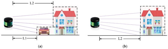
Figure 5.
(a) When the vehicle drives past the building and blocks the view of the LiDAR, the nearest distance of the point cloud in the red area from the sensor is L2, while the nearest distance of the point cloud in the green area from the sensor is L1. (b) After the vehicle moves away, the closest distance between the sensor and the point cloud in the green area is restored to L2, thereby indicating the presence of the building point cloud behind the car point cloud. Based on this, the car can be identified as a dynamic object.
Early studies proposing the use of the visibility-based approach to detect dynamic objects focused on iteratively updating the state of map points by successively fusing multiple measurements and checking the visibility between the query scan and the map [40,62]. In [40], the point cloud in the priori map is directly transformed to the query scan coordinate system. A point in the priori map is judged to be dynamic if it is crossed by the optical path of a point in the query scan. Given the difficulty in distinguishing dynamic points based on a single crossing, this method proposed a Bayesian probability-based model that leverages multiple pieces of information, such as the normal vector of a point, the distance between two points, and the category of the previous cycle, to calculate a probability that determines whether a point is dynamic or static. This work also represents a seminal contribution to the field of Long-term SLAM. Ambrus et al. constructed and maintained the static structure of the office space, namely the meta-room [62], through multiple observations and iterative improvement of new data. They employed RGB-D cameras to capture data from the environment, which enabled the accurate reconstruction of static structures by eliminating dynamic elements and incorporating previously occluded objects. One challenge of the visibility-based approach lies in identifying associations between query points and map points. The estimated pose of the LiDAR motion may contain errors that impact the accuracy of these associations, leading to the erroneous removal of static points. Regarding this issue, these methods assumed that the correct pose or registration was provided [62] or used a fixed-size association rule (e.g., within 1°) [40]. However, it is clear that both of these types of assumptions lack some degree of accuracy.
In [35], dynamic points were identified by selecting two reference scans and verifying whether potential dynamic points in the former reference scan were crossed (visible or not) by the laser beam of the latter reference scan. However, this method also assumed that the poses of the scans were given by SLAM, which would theoretically work better in the cases of denser LiDAR beams. Meanwhile, Qian et al. [63] proposed a dynamic SLAM framework based on LIO-SAM [23], RF-LIO, which utilizes a tightly coupled LiDAR-inertial odometry, adds adaptive multi-resolution range images, removes dynamic objects first for the acquired current LiDAR scan based on the visibility, and then employ scan matching. This approach exhibits good dynamic point cloud rejection capability in highly dynamic environments. Both [35] and [63] belong to the category of online real-time dynamic point cloud filtering (explained in detail in Section 3 below), which provides excellent real-time performance. However, the smaller number of scans selected and referenced can lead to slightly poorer accuracy in dynamic point cloud filtering.
On the other hand, Kim et al. used SLAM techniques to obtain an a priori map of the whole environment and then filtered dynamic target points from the point cloud based on the visibility principle [34]. A key challenge associated with the visibility-based approach is the potential erroneous removal of static points. Such errors can arise from factors such as the nature of the object itself (e.g., ground points with large incidence angles or points situated on the edges of object contours and elongated objects) or the lack of accuracy in the poses obtained via SLAM during the coordinate transformation of query scans and maps. In [34], these false positives are mitigated through the construction of multi-resolution range images. This study is a representative work utilizing the visibility-based approach, and its implementation and optimization will also be analyzed in detail in Section 3.
In recent years, significant progress has been made by integrating the visibility principle with semantic segmentation techniques for point clouds. Chen et al. proposed the LiDAR-MOS framework [64], which enables real-time detection and filtering of dynamic objects. Their approach utilizes three classical point cloud segmentation networks, namely RangeNet++ [65], SalsaNext [66], and MINet, to project the point cloud as distance images and compute residuals between the current and previous scans based on the visibility. These residual images are then combined with the current distance image and used as inputs to a fully convolutional neural network. The network is trained with the binary label to effectively distinguish between moving and stationary objects. Compared to Kim et al.’s method, this approach has the advantage of not relying on the pre-constructed map and operates online using only past LiDAR scans, resulting in improved real-time performance. However, one potential drawback is that it might miss some dynamic objects that are temporarily stationary for a certain period of time.
In Section 2.2, the paper discusses various works based on the visibility-based approach, as summarized in Table 3. The visibility-based approach is found to significantly reduce computational costs compared to the ray-tracing-based approach. However, the method faces limitations such as the challenge of ensuring uniform accuracy of the viewpoint, as well as the difficulty of occlusion and recognizing large dynamic objects in the absence of static objects behind them.
Table 3.
Visibility-based approach.
2.3. Segmentation-Based Approach
This approach aims to eliminate dynamic objects as a whole by identifying their categories. The idea is simple: if it is possible to accurately identify which points belong to pedestrians, vehicles, bicycles, or others then the dynamic point cloud can be easily filtered out. In recent years, machine learning techniques have been widely used in segmentation-based methods [67,68]. This method uses semantic segmentation based on deep learning to label the class of dynamic objects so that the dynamic point cloud can be eliminated directly with a bounding box, as shown in Figure 6. However, this approach heavily relies on supervised labels and they are vulnerable to labeling errors or dynamic objects of unlabeled classes [69].
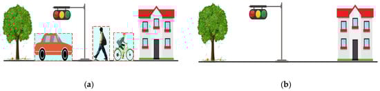
Figure 6.
(a) Dynamic objects are accurately identified for their respective categories, such as vehicles, pedestrians, or cyclists, and the detection bounding box is formed around them to segment the dynamic point cloud; (b) the point clouds inside the bounding box are removed to obtain a static scene model.
Early works on the segmentation-based approach did not incorporate machine learning techniques. Petrovskaya et al. modeled vehicles using a 2D bounding box and processed it in 2D representation for application it to 3D data [70]. However, early studies relied on manual model crafting rather than the learning-based approach, and they were insufficient in ensuring the efficiency and accuracy of removing dynamic objects, especially in complex, cluttered scenes with a richness of diverse dynamic objects.
There is also a part of early research using static 3D laser sensors for dynamic object point cloud segmentation. Kaestner et al. proposed a generative object detection algorithm that could extract objects of different sizes and shapes from observation data in an unsupervised manner [71]. In [72], Shackleton et al. used 3D grids for the spatial segmentation of point clouds, followed by point cloud surface matching using “spin images,” Kalman filtering-based tracking-assisted classification, and background subtraction-based background segmentation for object segmentation. Additionally, Anderson-Sprecher proposed using the accessibility analysis-evidence-grid background subtraction method [73], which uses accessibility analysis to remove the internal regions of objects and then performs background subtraction to detect foreground objects. However, these methods are not suitable for mobile 3D laser sensors and only focus on dynamic object segmentation and tracking from laser data, ignoring map updates.
Subsequent point cloud segmentation methods have gradually shifted towards the clustering-based approach. Litomisky first used the RANSAC (Random Sample Consensus) algorithm to eliminate large planes [74], then used VFH (Viewpoint Feature Histogram) to differentiate between static and dynamic clusters, and ultimately identified dynamic points by calculating the Euclidean distance between clusters. Yin leveraged feature matching to identify pixel correspondence between two images [75], detected prospective dynamic objects by performing pixel image subtraction, and then applied the Euclidean clustering method to extract clusters from dynamic objects as seeds. Yoon et al. proposed a region growth-based strategy to obtain dynamic clustering from confirmed dynamic points [35]. Despite the usefulness of clustering methods, they are still prone to omitting outlier dynamic points.
As relevant technologies continue to evolve, more and more studies are utilizing 3D point cloud data obtained from LiDAR scans as input for neural networks that output specific detection results to identify dynamic objects. Chen et al. proposed a method for dynamic object detection based on a multi-view 3D network that employs two sub-networks: one for 3D candidate box generation and the other for multi-view feature fusion, thus achieving the goal of 3D object reconstruction [76]. Zhou proposed a voxel encoding method for extracting features from point cloud data [77]. By encoding the point cloud into a voxel array and using 3D CNN(Convolutional Neural Network) for feature extraction, the study achieved an end-to-end learning process for 3D object detection based on point clouds. Similarly, Shi segmented point clouds using the PointNet++ network to generate a small number of high-quality 3D object candidates [78]. The RPN(Region Proposal Network) is utilized to generate reliable 3D object proposals for multiple classes. Using these proposals, the second stage detection network performs accurate orientation regression to predict the range, orientation, and class of objects in 3D space. Ruchti proposed using a neural network to predict the probability of a 3D laser point reflecting a dynamic object [79], determine whether each point belongs to a dynamic object by the prediction result, remove the points classified as dynamic objects, and then give only the remaining static points to SLAM for mapping and localization work. However, the disadvantage of neural network-based dynamic object removal methods is that they cannot detect untrained objects, and they occasionally fail to detect objects.
While many previous approaches were based on detecting actual motion, recent advancements in deep learning have enabled a shift toward appearance-based methods for dynamic object detection. In urban environments, it is often assumed that pedestrians, cyclists, and cars are the most common types of dynamic objects, and these classes can be detected in point clouds using a deep learning-based semantic segmentation approach. As reported in [80], a new SURF(Speeded Up Robust Features) algorithm was proposed that combines convolutional neural networks to extract semantic information from LiDAR 3D measurement point clouds to build maps with labeled surface elements that contain semantics. The algorithm employs a filtering algorithm for dynamic object removal, retaining static environmental information in the built semantic maps. Zhao et al. developed a semantic segmentation network using a dense matrix coding method to convert sparse [81], irregularly scanned LiDAR point clouds into a dense matrix. In [65], a rotating LiDAR sensor model was used to map single-frame point cloud data to the sensor coordinate system, resulting in a continuous range image. A CNN was then used to combine the range images for semantic segmentation to achieve recognition and segmentation in the point cloud. Wu et al. proposed an end-to-end pipeline, named SqueezeSeg [82,83], which transforms LiDAR point clouds into an image format and feeds them into a CNN. The CNN outputs a pixel-labeled map, which is then refined by a CRF(Conditional Random Field) recursive layer. Finally, a conventional clustering algorithm is utilized to obtain instance-level labels. Similarly, Biasutti proposed an end-to-end network for the semantic segmentation of 3D LiDAR point clouds based on U-Net [84]. This network extracts higher-order features of 3D neighbor points for each point and the learned features are then used to perform semantic segmentation using a U-Net segmentation neural network. Additionally, Cortinhal proposed the SalsaNext method [66], which uses a new context module and a residual dilated convolution structure to enhance segmentation accuracy by adding perceptual field and pixel rearrangement layers. However, these supervised learning approaches require manual labeling of training data, which can be costly and challenging to obtain. Moreover, they are limited to the subset of object types that exist in available datasets [10,85,86,87], thus hindering the ability to detect new dynamic objects.
The semantic segmentation of point cloud data based on appearance can identify potentially dynamic objects. However, this method does not necessarily indicate whether the objects are moving or stationary. For instance, an identified vehicle could be parked or in motion. Depending on the different needs for 3D point cloud models, it may be necessary to either remove parked vehicles or retain them. However, pure point cloud semantic segmentation methods tend to prioritize dynamic point cloud removal without distinction in the present moment, so they are combined with some traditional methods at times. Yu et al. combine semantic segmentation network and movement consistency checking to select moving and immobile points [46]. This method calculates the movement consistency of feature points and uses the proportion of moving points in the same object to determine whether the object is moving or stationary. Finally, dense semantic octo-tree maps are constructed using methods such as crawling algorithms. Sun et al. express the map in the form of an OctoMap and model each cell as an RNN(Recurrent Neural Network) to implement a Recurrent-OctoMap [88]. To extend the observation period of the Recurrent-OctoMap, the approach also develops a robust 3D localization and mapping system for continuously mapping dynamic environments. Meanwhile, Chen et al. combined the visibility-based approach with point cloud segmentation, the range images and residual images are used to train a CNN [64], producing a binarized label for each measurement indicating whether it belongs to a moving or static object. The specific content of their method is introduced in Section 2.2.
In recent work, Mersch et al. introduced an innovative concept involving the application of sparse 4D CNN to extract spatio-temporal features and to segment points into moving and non-moving [89]. To enhance the precision and recall of moving object segmentation, they employed a voxelized binary Bayesian filter, which provides a probabilistic representation of dynamic environments. He et al. introduced an end-to-end sparse tensor-based CNN [90]. Their method leverages the AR-SI theory [91] to create an autoregressive system-identification filter that discerns moving objects in a 3D point cloud, providing temporal features for CNN inputs. Subsequently, the temporal features are combined with special features extracted from the original point cloud. By mapping the labels to segmentation training, the method produces accurate IoU results. Toyungyernsub et al. proposed an integrated framework for static-dynamic object segmentation and local environment prediction [92]. This framework utilizes an occupancy-based environmental representation and incorporates modules for static-dynamic object segmentation and environment prediction. The static-dynamic object segmentation module employs the SalsaNext [66] neural network architecture to detect static and moving objects within the environment. The environment prediction module utilizes the predicted static-dynamic segmentation output as input to forecast the future occupancy state of the environment. It is worth noting that, despite the promising results yielded by [46,64,88], these methods still require manually labeled, high-quality datasets.
In Section 2.3, this paper delves into the implementation of various algorithms based on the segmentation-based approach and explores their strengths and limitations, which are summarized in Table 4. In general, deep learning-based semantic segmentation methods can effectively and efficiently detect dynamic targets in point clouds and filter them out. However, one major limitation is that they can only recognize pre-trained dynamic object types, and other types of dynamic objects cannot be detected. Additionally, the requirement of GPU resources for deep learning-based methods results in a higher cost.
Table 4.
Segmentation-based approach.
2.4. Other Approaches
There exist several other methods for filtering out dynamic point clouds in a 3D point cloud, which are based on specific assumptions and have achieved good results in certain scenarios. In this section, these methods will be introduced. However, it is important to note that these methods are not systematic and rely on certain conditions and constraints.
In [93], an approach for joint self-localization and generic object tracking is proposed, which integrates object detection and tracking with sensor trajectory estimation. The method involves pre-processing the collected 3D point cloud, computing features, and generating object hypotheses, followed by generating a trajectory for each hypothesis and tracking them over time. Trajectories that exhibit consistency are labeled as dynamic by the learned classifier. However, a limitation of this method is that it assumes that objects can be tracked continuously in subsequent scans, which may not hold for some dynamic objects in real scenes, such as pedestrians.
An alternative approach was proposed by Dewan’s team [94,95], who used rigid scene flow, i.e., point-wise velocity estimation, to detect dynamic objects. They compared subsequent point clouds and identified motion sequentially using a voting scheme. The first detected motion will always be the relative motion of the stationary environment, followed by the largest dynamic objects. Motion cues were used for the segmentation and tracking of moving objects, and point-level matching was performed between successive scans. Their work was compared with that of [93] and was shown to have superior performance. However, the method requires prior rejection of ground points in the pre-processing step, and relies on the minimum velocity assumption, making it difficult to distinguish the scene stream from the noise for slow-moving dynamic objects. Therefore, it is also unsuitable for filtering out pedestrians.
In [96], a scan-to-model-based matching framework is proposed that uses the localized LiDAR scan of the previous region as a model with an IMLS(Implicit Moving Least Squares) surface representation, which is known for its good approximation and smoothness, and for its superior noise and outlier reduction. The method has demonstrated good performance in KITTI benchmark tests with excellent low-drift characteristics. However, the method assumes that all objects smaller than a certain size are potentially dynamic objects, which may result in the loss of valuable features for matching or 3D reconstruction.
Ushani et al. proposed a learning-based method to compute scene streams that use 3D LiDAR sensor data to construct the occupancy grid [97], extract foregrounds through a learned background filter, and use the filtered occupancy grid to compute the original scene stream between successive scans to roughly identify dynamic point cloud, which is then refined by a learned classifier. However, as the method assumes that the motion of dynamic objects is restricted to a horizontal plane and only constructs the occupancy grid of 50 m × 50 m, it is clearly not suitable for dynamic detection over large areas.
Lim et al. proposed an innovative method for detecting and filtering a dynamic point cloud in a 3D point cloud based on the prior assumption that the majority of dynamic objects might be in contact with the ground [31]. Similar to the visibility-based approach, this work identifies dynamic objects by comparing the difference between query scan and submap. However, this method divides the scanned spatial region into bins and compares the height difference of the point cloud in the z-direction within each bin. If the ratio of the extreme height difference within a bin is below a certain threshold, it is inferred that dynamic objects are present, and all points above the ground points in this bin are removed. This method has overcome many limitations of the ray-tracing-based approach [33] and the visibility-based approach [34], as discussed in detail in Section 3. However, it assumes that dynamic objects are in contact with the ground, and it may encounter a higher risk of failure in more complex dynamic environments.
Wang et al. also proposed an approach to distinguish between dynamic and static points using the vertical voxel height descriptor [98], but the key distinction is that their method does not rely on a complete global map and enables online real-time processing of dynamic point cloud. In their system, akin to RF-LIO [63], the IMU data is pre-integrated to obtain initial attitude outputs, then the pre-processing module involves feature extraction and segmentation of scans, and local map construction. The dynamics removal module employs the vertical voxel occupancy descriptor to filter out dynamic objects and performs matching between scans and the submap to achieve accurate attitude estimates. However, this kind of method that relies on vertical descriptors to identify dynamic objects inevitably has inherent limitations, leading to compromised localization accuracy and robustness when dealing with sloping pavements.
In Section 2.4, this study highlights the implementation ideas and problems of certain methods for filtering out a dynamic point cloud. These methods are summarized in Table 5. While these methods can provide better results than traditional approaches in certain scenarios, they are often based on subjective assumptions and lack sufficient robustness in complex and chaotic dynamic environments.
Table 5.
Other approaches.
3. Processing Strategies of Dynamic Objects in the SLAM Framework
Section 2 introduces different methods for filtering dynamic targets in a 3D point cloud in the solution-oriented dimension. In this section, this paper explores the problem-oriented dimension and investigates different processing strategies that correspond to different categories of dynamic objects in the SLAM framework. Initially, an overview of the SLAM system framework had been provided before objects have been classified into four categories based on their dynamic characteristics: high dynamic objects, low dynamic objects, semi-dynamic objects, and static objects. For different categories of dynamic objects, three distinct processing strategies have been summarized: Online real-time filtering, Post-processing after the mapping, and Long-term SLAM. The paper also performs a detailed analysis of different methods within the same processing strategy.
3.1. The Overall Framework of the SLAM System
SLAM technology has made significant strides over the past few decades. As far back as 1992, the feature-based fusion SLAM framework [99] was established. The SLAM framework based on 3D LiDAR primarily organizes the SLAM according to its functionality, namely, localization and mapping, as shown in Figure 7. As SLAM technology has developed, localization and mapping have evolved from two distinct modules into a comprehensive system. The two modules promote each other. The high-precision odometer composed of multiple sensors provides real-time pose estimation for the robot and the basis for the reconstruction and stitching of the 3D scene. Similarly, high-precision 3D reconstruction provides important data for pose estimation for feature-based odometry. Even a separate odometer system is also inseparable from the establishment or storage of temporary local maps to assist pose estimation [100].
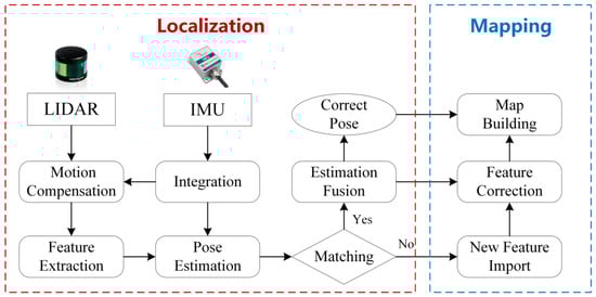
Figure 7.
The basic framework of SLAM based on 3D LiDAR.
In terms of components, the modern SLAM system based on 3D LiDAR can generally be divided into two stages: the front-end and the back-end, as illustrated in Figure 8. The front-end is responsible for the real-time collection of raw data from the environment, feature extraction and matching, pose estimation for the current scan, and storage of corresponding local map information. Meanwhile, the back-end is primarily responsible for loop closure detection, triggering global drift correction, and optimizing pose estimation for large-scale 3D scene reconstruction. Precisely because the front-end and back-end belong to different stages with different roles and receive and process different data and information, different processing strategies exist in the SLAM framework based on 3D LiDAR for different classes of dynamic objects.
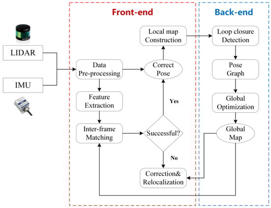
Figure 8.
The main components of the SLAM system based on 3D LiDAR.
3.2. Classification of Objects Based on the Dynamic Degree
In the SLAM framework, the LiDAR scans point clouds of various objects, most of which are permanent static objects that need to be retained for subsequent feature matching, pose estimation, and mapping, but there are also many dynamic objects that, due to their different degrees of dynamics, have different processing strategies. For instance, while vehicles are dynamic objects, vehicles driving on the road, waiting for traffic lights, and parked in parking lots are clearly separate categories of dynamic objects requiring different processing strategies in the SLAM framework. In certain studies, dynamic objects are often categorized into two broad groups: high dynamic (HD) and low dynamic (LD) [101]. However, this classification may lack precision, resulting in a potential compromise on accuracy and efficiency during the subsequent filtering process. This paper proposes a more refined classification of objects based on the degree of their dynamics, dividing them into the following four categories:
- High dynamic objects: objects that move continuously in the LiDAR scan, such as people walking on the street, moving vehicles, and running pets.
- Low dynamic objects: objects that are in a transient state, such as people standing on the street talking, and vehicles stopped waiting for a traffic light.
- Semi-dynamic objects: objects that remain stationary during a SLAM cycle, but not forever, such as vehicles in the parking lot, stacked materials, temporary sheds, temporary fences, temporary stages, and mobile catering vehicles on the roadside.
- Static objects: objects that are permanently immobile, such as walls, buildings, and structures, roads, traffic signals, and the vast majority of fixed facilities.
The first three types of objects can be collectively referred to as dynamic objects, and for different categories, different stages of processing strategies can be used in the SLAM framework. For example, high dynamic objects can be filtered out online in real-time, while low dynamic objects may be rejected using post-processing after the mapping. Meanwhile, semi-dynamic objects necessitate the use of Long-term SLAM to detect changes between different sessions of SLAM. It is worth noting that these four types of strategies are upwardly compatible. For instance, Long-term SLAM can also filter out high and low dynamic objects with greater accuracy, but the real-time performance decreases due to the increased information required for reference and comparison.
3.3. Online Real-Time Filtering out of Dynamic Objects
This strategy focuses on the online filtering of dynamic objects during SLAM based on 3D LiDAR, ensuring real-time availability of a static model of the entire scene while the SLAM is being completed. It offers the advantage of excellent synchronization and real-time performance. However, due to the limited amount of data that can be referenced and compared, which are typically only adjacent scans from a short period of time before and after the current scan or local submaps comprising these recent scans, the effectiveness of the strategy in rejecting dynamic objects is limited. Consequently, this strategy is primarily suitable for filtering high dynamic objects in the scene.
As mentioned in Section 3.1, during the LiDAR-based SLAM framework, the front-end is responsible for aligning point clouds between different scans, while one of the functions of the back-end is to perform the construction of the overall 3D model of the scene. The strategy of online real-time filtering out of dynamic objects can be implemented either in the front-end during the registration or in the back-end during the mapping.
Currently, mainstream point cloud alignment methods are based on the assumption of a static background. Ideally, it is best to filter out dynamic objects before or during the front-end alignment to ensure that the final result is based on static point clouds. In SLAM based on 3D LiDAR, research on rejecting dynamic objects during front-end alignment is relatively limited. The approaches are generally divided into two types: traditional methods and deep learning. Traditional methods often rely on inter-scan comparison to separate dynamic points, such as eliminating points that are too far away or comparing differences between the current scan and submap. In contrast, deep learning-based methods can directly detect dynamic objects based on their categories from the point cloud and remove them before alignment, which is faster and more accurate.
Qian et al. proposed a method based on the visibility-based approach, RF-LIO [63], which filters out dynamic points prior to scan matching. Their method builds upon the LIO-SAM [23] framework, with the addition of range image construction and dynamic point rejection. Upon a new scan arrival, an initial position estimate is obtained using IMU odometry, and an initial resolution is determined. This resolution is then used to construct the current scan and the corresponding submap as range images, which are compared based on visibility to detect the dynamic points in the submap for removal. RF-LIO is a traditional method for rejecting dynamic points at the front-end of SLAM, but due to the limited number of scans available for comparison, it can only be used to filter out high dynamic objects, and its application scenario is limited by the shortcomings of the visibility-based approach.
Pfreundschuh et al. present a deep learning-based approach to reject dynamic point clouds in the front-end [102], which is gaining popularity compared to conventional methods. The method combines traditional dynamic point cloud filtering methods with deep learning point cloud segmentation. It starts by constructing an automatic tagging pipeline based on the concept of ray-tracing-based dynamic point cloud detection, which is used to generate a dataset for training and testing. Then, 3D-MiniNet is trained with this dataset to obtain an end-to-end network, which directly segments the dynamic objects in the original point cloud. Finally, the clean point cloud after filtering is provided to LOAM [20] for subsequent SLAM works. This approach presents an unsupervised generic dynamic object-aware LiDAR SLAM method, which significantly reduces the cost of manual tagging in the dataset and human interference and improves the accuracy of dynamic object rejection. However, a common issue with learning-based methods is that dynamic objects that belong to untrained classes cannot be recognized.
In most real-life scenes, dynamic objects usually do not cause significant interference during point cloud alignment, but their presence can lead to the ghost-trail effect that can greatly impact the mapping stage. So it is more common to perform online real-time filtering out of dynamic objects during the mapping in the back-end. Various methods are used to handle dynamic points in key frames inserted into the map in real-time, resulting in a clean 3D scene map that can be obtained while the mapping is completed. Several works have utilized the real-time filtering of dynamic objects during the mapping of SLAM, including [51,53,54,55,94,95], among others. Two studies employing this strategy are presented below.
In [35], a concise idea was proposed where one scan is taken as a reference frame before and after the query scan. The front reference scan is used to compare the point-to-point distance, and the points with too large a distance are identified as potential dynamic points, which are then put into the back reference scan for verification, and if they are crossed by the laser beam of the back reference scan, they are confirmed as dynamic points. The confirmed dynamic points are used as seeds to grow clusters and obtain dynamic clusters. The whole process of dynamic point cloud filtering does not require constructing local maps or submaps, only two reference scans.
Fan et al. present a recent study that uses the real-time filtering out of dynamic objects strategy [103]. The method starts with an initial screening of dynamic targets using the visibility-based approach to enhance the efficiency of subsequent computations. The static submap MS obtained after initial screening is then optimized online during back-end mapping to obtain accurate dynamic point cloud filtering results. The core idea of the back-end algorithm is based on the ray-tracing-based approach. The voxels are marked as free when light passes through them, and a visibility check is introduced to approximate the denominator nfree of the occupancy probability, which is the number of light rays passing through each voxel. This process speeds up the ray-tracing process and greatly reduces computational resource consumption.
In Section 3.3, the paper presents the first strategy for processing dynamic objects in SLAM based on 3D LiDAR: Online real-time filtering out of dynamic objects. The relevant methods are summarized in Table 6. This strategy has the advantage of being synchronized with SLAM, which has excellent real-time performance without requiring additional time. However, the downside is that in order to achieve real-time filtering, only a limited number of reference scans are used, which may result in significant differences between subsequent point cloud comparisons due to occlusion or sparse data. As a result, this strategy is only suitable if filtering accuracy is not highly demanding, and it is only applicable to high dynamic objects.
Table 6.
Different methods using the online real-time filtering out of dynamic objects strategy.
3.4. Post-Processing of Dynamic Objects after the Mapping
This strategy involves post-processing to filter out dynamic objects after the completion of the SLAM mapping, in conjunction with the overall map of the 3D scene. It can refer to all the scanned point clouds in the entire SLAM cycle, making it more conducive to the detection of temporarily immobile objects (i.e., low dynamic objects) and of course, the identification of high dynamic objects is even easier. The post-processing strategy can achieve more accurate and thorough filtering of dynamic objects, but the drawback is that the dynamic objects filtering lags after the SLAM mapping, resulting in a further time delay after SLAM before the final static map is available.
Numerous studies have adopted the strategy of post-processing after mapping because it considers the information of all global scans and enables accurate and thorough dynamic filtering. Early works include [38,40,52,104,105], while recent works include [31,32,33,34,106,107], and others. Despite using the same post-processing strategy, these studies have employed different methods for filtering dynamic point clouds. The paper has selected three different methods that were applying this strategy, providing detailed analyses of their algorithmic principles, implementation process and optimization ideas.
The peopleremover method [33] is a post-processing filtering of dynamic point cloud method using the ray-tracing-based approach, whose main contribution is to provide effective optimization for the false positives (i.e., static points are incorrectly identified as dynamic points for removal) and false negatives (dynamic points in the static grids are incorrectly retained). The concept of the proposed algorithm lies in the storage of information in each voxel, which is the ID of all scans that have hit that voxel rather than the number or probability. This optimization significantly reduces the amount of data to be stored. The ray-tracing-based approach is prone to producing false positives in certain local special cases, such as ground points or corner points. This is due to challenges such as excessively large angles of incidence or occlusion. To overcome these, this work proposes a “maximum safe distance” approach. For a given laser point, traversal of all grids on its optical path is halted prematurely once it reaches a specified distance from the point, ensuring that the static grids near the point are not mistakenly marked as dynamic. For false negatives as shown in Figure 9, the left image displays point cloud-obtained scans of a person standing on the ground, consisting of person points and ground points. Filtering of the dynamic points produces a point cloud as depicted in the middle image, where the three red points situated above the ground are evidently dynamic (i.e., person points) but are erroneously retained. To address this issue, this work proposes an approach. During the process of marking the dynamic grid, the IDs of scans that hit it are examined in the adjacent voxels, and if present, the point clouds of the scans corresponding to these IDs in the adjacent voxels are removed. In the right image, the ID of the scan that generates red points is stored in the B2 and C2 grids, so that the red points in the adjacent B1 and C1 grids are also filtered out.
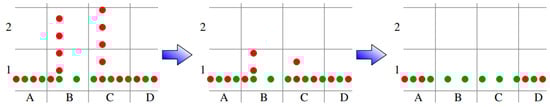
Figure 9.
Optimization of false negatives in the peopleremover method.
The Remove, then Revert approach [34] proposes the post-processing strategy based on visibility to filter out dynamic point clouds. This method adopts the multi-resolution range image to address the false-positive problem that is commonly encountered in the visibility-based approach. The optimization ideas presented in this study have been referenced in subsequent studies. A set of original neighboring scans and their corresponding transformed poses to the global map (SE(3)) are given. A scan from this set is designated as the query scan, denoted as PQ, while all other scans are consolidated into a submap, denoted as PM. PQ and PM are converted to the same coordinate system and then projected as range images. If a point in PM is shallower in depth than its corresponding point in PQ, it is identified as a dynamic point and eliminated. The points in PM can be divided into two categories: the dynamic point set D1 and the static point set S1, and D1 contains both true and false positives. The study found that using range images of lower angular resolution resulted in a significant reduction in false positives, and it takes advantage of this property to propose a two-step method. First, the most rigorous dynamic point deletion is performed using the highest resolution range images, and this yields a preliminary dynamic point set and a static point set. Then, the image resolution is reduced and re-matched to revert the points that were previously considered dynamic but are now considered static points to the static point set. This process is repeated for all scans and resolutions until the final static map is obtained. The pipeline of this algorithm is depicted in Figure 10:
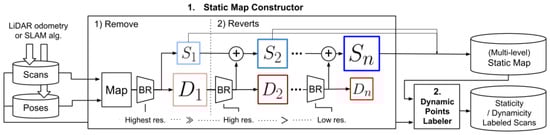
Figure 10.
The pipeline of the Remove, then Revert method.
ERASOR [31] is a method of post-processing for filtering out dynamic point clouds based on dynamic objects in contact with the ground, effectively overcoming the limitations of the ray-tracing-based and visibility-based approaches. This work considers that most dynamic objects make contact with the ground, so if the points are present above ground points in PM but not in PQ at the same location then they can be classified as dynamic objects. The specific method involves the creation of a spatial region in both the PQ and PM, referred to as the Volume of Interest (VOI). This region is then divided into bins based on specific angles and radii, and the differences between the point clouds above the ground points in the PQ and PM are then compared within each bin. This method introduces a descriptor called the Region-wise Pseudo Occupancy Descriptor (R-POD), which is utilized to represent the height difference in the z-direction of the point cloud in each bin. Moreover, the work proposes an operation known as the Scan Ratio Test (SRT), which identifies possible dynamic regions by comparing the difference in descriptors calculated for bins at the same location in the PQ and PM. The operation calculates the ratio of the two descriptors, and the bin with a ratio less than the threshold value is identified as a potential dynamic region while other regions are preserved. The final step is to fit ground points within all the bins marked as dynamic regions, and then remove all points lying above the ground points as dynamic points. The ground extraction method used was R-GPF(Region-wise Ground Plane Fitting). The eigenvalues and eigenvectors of the ground points were calculated using PCA(Principal Component Analysis), then the plane equation of the ground was calculated and the points above the ground were removed as dynamic points. Finally, dynamic bins that had been processed were combined with the static bins that were preserved previously, resulting in a global static map. An overview of this work is illustrated in Figure 11:
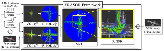
Figure 11.
Overview of the ERASOR method.
In Section 3.4, the paper presents the main ideas of the post-processing strategy and of several different methods that employ it. The advantages and disadvantages of each method are also summarized in Table 7. Overall, the post-processing strategy is the most widely used tactic because it does not require real-time considerations and can use all scans in the entire SLAM cycle as reference information to identify dynamic objects, which is more accurate for dynamic point cloud filtering. The post-processing strategy can filter out both high and low dynamic objects, making it ideal if high dynamic object rejection accuracy is required. However, the proposed strategy may not be applicable to scenes with a very high percentage of dynamic objects, as it becomes challenging to obtain accurate poses between each scan and the global map in such scenarios. In addition, the specific method used to filter out dynamic objects in this strategy needs to be carefully selected based on the scene characteristics.
Table 7.
Different dynamic point cloud filtering methods using post-processing strategy.
3.5. Long-Term SLAM
The two strategies presented above occur at different stages within a SLAM cycle, but semi-dynamic objects are typically stationary and undetectable throughout a single SLAM cycle. However, in many application scenarios, it is necessary to maintain a long-term model of the environment, which requires filtering out these semi-dynamic objects. Long-term SLAM is a strategy that detects and removes changed objects between different SLAM cycles while updating and maintaining the environment map. As an emerging field of SLAM research, the measures used to detect and filter out dynamic objects in Long-term SLAM remain similar to those described in Section 2. The uniqueness of this strategy is in the temporal and spatial alignment and fusion of trajectories and maps from different SLAM cycles, as well as the updating and maintenance of the long-term 3D scene map.
Pomerleau et al. presented seminal research in the field of Long-term SLAM [40]. The authors argue that the core of map fusion in Long-term SLAM lies in how to handle the parts of the map that change between different sessions, i.e., high and low dynamic objects and semi-dynamic objects. Their dynamic object detection and filtering method is based on visibility, but instead of using range images, they transform the point cloud in the map directly into the query scan coordinate system. Dynamic points are initially filtered based on whether the points in the map are crossed by the light paths of the points in the query scan, and information from multiple sources is fused to further identify dynamic objects in the map that need updating. This work is significant as it unifies dynamic object filtering and map updating in LiDAR-based SLAM, serving as an important guideline for future Long-term SLAM research. However, the authors’ assumption of precise poses between each query scan and map may not hold in real outdoor environments.
In previous years, several Long-term SLAM studies have proposed using different map representations such as NDT(Normal Distribution Transformation) maps [108], occupancy grid maps [14,88,109], or frequency domain representation [110]. Einhorn presents a generic SLAM method that can be used for both 2D and 3D scenes [108]. It combines the occupancy grid map with the NDT map and modifies the NDT mapping method to better handle free-space measurements and dynamic object detection. This method is both a SLAM mapping algorithm and supports localization and map updates. Another study proposes an online update method for 2D grid maps that uses a graph-based SLAM system to anchor local maps [109], then combines occupancy estimates from multiple local maps to produce a global occupancy map. To handle too many local maps to maintain the quality of the global rendered map, the employed method prunes redundant local maps using algorithms that determine their cost and contributions. However, for change detection in 3D environments, dealing directly with a raw 3D point cloud may be preferred over dealing with other forms of maps.
One of the most recent studies using Long-term SLAM is presented in [4,101]. The former introduces the concept of sessions, where the first map build belongs to session zero, and an a priori map of the current environment is constructed and stored in the database. When the robot performs a task, it enters localization mode, where each localization reads the map data from the database and creates a new session. The old submap is continuously pruned to limit its number, and the new submap is added to the global map of the current session. When the old submap is deleted, sparsification of the pose optimization is triggered. Finally, at the end of the localization task, the updated map is saved and passed into the database, thus completing a map update. As can be seen, the focus of this study is not on detecting dynamic objects during Long-term SLAM, but rather on updating the map in real-time to guide the current motion of the robot, which has good applications in highly dynamic places such as supermarkets and shopping malls.
In [101], the focus lies on map building and management in the context of Long-term SLAM, which involves detecting differences in SLAM between different sessions at different times and updating these changes to the central map. The authors propose a Long-term SLAM system, called “LT-mapper”, which comprises three sub-modules: LT-SLAM, LT-removert, and LT-map. The LT-SLAM module tackles the problem of trajectory alignment between multi-temporal SLAM by using the anchor node-based loop back factor, and ICP iterative computation is used to obtain the relative constraints between the corresponding keyframes of two different sessions to achieve the alignment between trajectories. The LT-removert module, based on the “Remove, then Revert” method, initially filters the dynamic objects HD (i.e., high and low dynamic objects) in a single session. For the dynamic objects LD (i.e., semi-dynamic objects) between different SLAM sessions, the kd-tree is constructed in the central map, and the neighborhood search is performed in the target point cloud in the query map. The “Remove, then Revert” method is again used for false positives in LD to further revert them to static points. Finally, the LT-map module’s task is to extract the HD and LD (i.e., all dynamic objects) from the change detection to form delta maps and to update the central map by uploading delta maps. By solving the problem of temporal and spatial alignment and integration of the trajectories and maps of different sessions of SLAM, LT-mapper effectively maintains a long-term 3D scene map.
In Section 3.5, the paper presents Long-term SLAM as the ultimate strategy for dynamic object filtering in SLAM based on 3D LiDAR, and the related works are summarized in Table 8. While Long-term SLAM is a more comprehensive and systematic approach than the other two strategies, its goals are not limited to detecting dynamic objects but rather encompass a range of core tasks such as long-term map updating and maintenance, as well as real-time robot localization, motion guidance, and map correction.
Table 8.
Related works for long-term strategy.
In Section 3, the paper categorizes objects based on their dynamic degree and summarizes three corresponding strategies for different classes of dynamic objects at different stages of SLAM based on 3D LiDAR. Table 9 summarizes the applicability and compares the pros and cons of the three strategies. It should be noted that the division of the different categories of strategy is problem-oriented, and the specific measures used in each are those dynamic point cloud filtering methods mentioned in Section 2: ray-tracing-based filtering, visibility-based filtering, segmentation-based filtering, and other approaches. Moreover, the algorithm principles of the corresponding methods selected for different strategies may be the same.
Table 9.
Different strategies for dynamic object filtering.
4. Conclusions and Future Outlook
Over the years, SLAM based on 3D LiDAR has made significant progress. However, most of the mainstream algorithms assume a static background, which is not the case in real-world scenes that are filled with various dynamic objects. These dynamic objects can cause interference and impact the front-end and back-end operations of SLAM, resulting in serious damage to its accuracy and robustness. Therefore, it is necessary to filter out the dynamic point cloud in SLAM based on 3D LiDAR and to obtain a clean 3D scene model.
This paper aims to classify and summarize various universal methods for filtering out dynamic point clouds in the 3D point cloud and different strategies for handling dynamic objects in SLAM based on 3D LiDAR. The dynamic point cloud filtering methods are solution-oriented, while the three processing strategies are problem-oriented, serving the practical applications of dynamic point cloud-removal technology within the realm of SLAM based on 3D LiDAR. From a broader perspective, all of these strategies, methods, and algorithms can be summarized under one keyword: change detection. Detecting changes between a scan and several scans, or between scans and the map is the key to filtering out high and low dynamic objects, whereas semi-dynamic object updating is the change detection between scans and maps of different SLAM cycles. This paper discusses how change detection is performed during SLAM based on 3D LiDAR and analyses the advantages and disadvantages of each study. However, this work is not exhaustive, and only a few representative studies are included to provide readers with a general understanding and a starting point for tackling similar problems.
In future research, dynamic point cloud filtering methods based on deep learning are poised to be a significant development direction. One proposal by [102] is the use of deep learning methods to train and generate datasets, and as related technologies advance, future object training will cover various categories in realistic scenes to achieve accurate identification of dynamic objects in the original point cloud at the front-end. This will provide SLAM with clean point clouds for alignment and subsequent works, thus improving and extending the performance and functionality of SLAM. Long-term SLAM is also a promising area for future research. The ultimate goal of SLAM is to enable autonomous robot operation or autonomous vehicle driving. Achieving accurate localization and operation in a dynamic environment that changes constantly, while judging the differences between the current environment and the priori map and correcting the map in real-time, will require Long-term SLAM. Further research and development of Long-term SLAM technology will be necessary to achieve this goal.
Author Contributions
Conceptualization, Z.Z.; methodology, H.P.; formal analysis, H.P. and Z.Z.; investigation, H.P.; resources, Z.Z.; writing—original draft preparation, H.P.; writing—review and editing, H.P., Z.Z. and L.W.; supervision, L.W.; project administration, L.W.; funding acquisition. All authors have read and agreed to the published version of the manuscript.
Funding
This study was funded by the National Key R&D Program of China, 2022YFC2904105 and 2023YFC2907305.
Institutional Review Board Statement
Not applicable.
Informed Consent Statement
Not applicable.
Data Availability Statement
Data are contained within the article.
Acknowledgments
The authors gratefully acknowledge the funders and all advisors and colleagues who supported our work.
Conflicts of Interest
Author L.W. was employed by the company Changsha Digital Mine Co., Ltd., China. The remaining authors declare that the research was conducted in the absence of any commercial or financial relationships that could be construed as a potential conflict of interest.
References
- Cadena, C.; Carlone, L.; Carrillo, H.; Latif, Y.; Scaramuzza, D.; Neira, J.; Reid, I.; Leonard, J.J. Past, present, and future of simultaneous localization and mapping: Toward the robust-perception age. IEEE Trans. Robot. 2016, 32, 1309–1332. [Google Scholar] [CrossRef]
- Shan, T.; Englot, B. Lego-loam: Lightweight and ground-optimized lidar odometry and mapping on variable terrain. In Proceedings of the 2018 IEEE/RSJ International Conference on Intelligent Robots and Systems (IROS), Madrid, Spain, 1–5 October 2018; pp. 4758–4765. [Google Scholar]
- Mur-Artal, R.; Tardós, J.D. Orb-slam2: An open-source slam system for monocular, stereo, and rgb-d cameras. IEEE Trans. Robot. 2017, 33, 1255–1262. [Google Scholar] [CrossRef]
- Zhao, M.; Guo, X.; Song, L.; Qin, B.; Shi, X.; Lee, G.H.; Sun, G. A general framework for lifelong localization and mapping in changing environment. In Proceedings of the 2021 IEEE/RSJ International Conference on Intelligent Robots and Systems (IROS), Prague, Czech Republic, 27 September–1 October 2021; pp. 3305–3312. [Google Scholar]
- Dey, E.K.; Awrangjeb, M.; Tarsha Kurdi, F.; Stantic, B. Machine learning-based segmentation of aerial LiDAR point cloud data on building roof. Eur. J. Remote Sens. 2023, 56, 2210745. [Google Scholar] [CrossRef]
- Wang, Y.; Lin, Y.; Cai, H.; Li, S. Hierarchical Fine Extraction Method of Street Tree Information from Mobile LiDAR Point Cloud Data. Appl. Sci. 2022, 13, 276. [Google Scholar] [CrossRef]
- Lim, H.; Hwang, S.; Shin, S.; Myung, H. Normal distributions transform is enough: Real-time 3D scan matching for pose correction of mobile robot under large odometry uncertainties. In Proceedings of the 2020 20th International Conference on Control, Automation and Systems (ICCAS), Busan, Republic of Korea, 13–16 October 2020; pp. 1155–1161. [Google Scholar]
- Kim, H.; Song, S.; Myung, H. GP-ICP: Ground plane ICP for mobile robots. IEEE Access 2019, 7, 76599–76610. [Google Scholar] [CrossRef]
- Behley, J.; Stachniss, C. Efficient Surfel-Based SLAM using 3D Laser Range Data in Urban Environments. In Proceedings of the Robotics: Science and Systems, Pittsburgh, PA, USA, 26–30 June 2018; p. 59. [Google Scholar]
- Behley, J.; Garbade, M.; Milioto, A.; Quenzel, J.; Behnke, S.; Stachniss, C.; Gall, J. Semantickitti: A dataset for semantic scene understanding of lidar sequences. In Proceedings of the IEEE/CVF International Conference on Computer Vision, Seoul, Republic of Korea, 27–28 October 2019; pp. 9297–9307. [Google Scholar]
- Kim, G.; Kim, A. Scan context: Egocentric spatial descriptor for place recognition within 3D point cloud map. In Proceedings of the 2018 IEEE/RSJ International Conference on Intelligent Robots and Systems (IROS), Madrid, Spain, 1–5 October 2018; pp. 4802–4809. [Google Scholar]
- Kim, H.; Liu, B.; Goh, C.Y.; Lee, S.; Myung, H. Robust vehicle localization using entropy-weighted particle filter-based data fusion of vertical and road intensity information for a large scale urban area. IEEE Robot. Autom. Lett. 2017, 2, 1518–1524. [Google Scholar] [CrossRef]
- Hawes, N.; Burbridge, C.; Jovan, F.; Kunze, L.; Lacerda, B.; Mudrova, L.; Young, J.; Wyatt, J.; Hebesberger, D.; Kortner, T. The strands project: Long-term autonomy in everyday environments. IEEE Robot. Autom. Mag. 2017, 24, 146–156. [Google Scholar] [CrossRef]
- Banerjee, N.; Lisin, D.; Briggs, J.; Llofriu, M.; Munich, M.E. Lifelong mapping using adaptive local maps. In Proceedings of the 2019 European Conference on Mobile Robots (ECMR), Prague, Czech Republic, 4–6 September 2019; pp. 1–8. [Google Scholar]
- Ye, H.; Chen, Y.; Liu, M. Tightly coupled 3D lidar inertial odometry and mapping. In Proceedings of the 2019 International Conference on Robotics and Automation (ICRA), Montreal, QC, Canada, 20–24 May 2019; pp. 3144–3150. [Google Scholar]
- Dube, R.; Cramariuc, A.; Dugas, D.; Sommer, H.; Dymczyk, M.; Nieto, J.; Siegwart, R.; Cadena, C. SegMap: Segment-based mapping and localization using data-driven descriptors. Int. J. Robot. Res. 2020, 39, 339–355. [Google Scholar] [CrossRef]
- Wang, J.; Wang, L.; Peng, P.; Jiang, Y.; Wu, J.; Liu, Y. Efficient and accurate mapping method of underground metal mines using mobile mining equipment and solid-state lidar. Measurement 2023, 221, 113581. [Google Scholar] [CrossRef]
- Zhang, J.; Singh, S. Low-drift and real-time lidar odometry and mapping. Auton. Robot. 2017, 41, 401–416. [Google Scholar] [CrossRef]
- Dubé, R.; Gawel, A.; Sommer, H.; Nieto, J.; Siegwart, R.; Cadena, C. An online multi-robot SLAM system for 3D LiDARs. In Proceedings of the 2017 IEEE/RSJ International Conference on Intelligent Robots and Systems (IROS), Vancouver, BC, Canada, 24–28 September 2017; pp. 1004–1011. [Google Scholar]
- Zhang, J.; Singh, S. LOAM: Lidar odometry and mapping in real-time. In Proceedings of the Robotics: Science and Systems, Berkeley, CA, USA, 12–16 July 2014; pp. 1–9. [Google Scholar]
- Lin, J.; Zhang, F. Loam livox: A fast, robust, high-precision LiDAR odometry and mapping package for LiDARs of small FoV. In Proceedings of the 2020 IEEE International Conference on Robotics and Automation (ICRA), Paris, France, 31 May–31 August 2020; pp. 3126–3131. [Google Scholar]
- Wang, H.; Wang, C.; Chen, C.-L.; Xie, L. F-loam: Fast lidar odometry and mapping. In Proceedings of the 2021 IEEE/RSJ International Conference on Intelligent Robots and Systems (IROS), Prague, Czech Republic, 27 September–1 October 2021; pp. 4390–4396. [Google Scholar]
- Shan, T.; Englot, B.; Meyers, D.; Wang, W.; Ratti, C.; Rus, D. Lio-sam: Tightly-coupled lidar inertial odometry via smoothing and mapping. In Proceedings of the 2020 IEEE/RSJ International Conference on Intelligent Robots and Systems (IROS), Las Vegas, NV, USA, 25–29 October 2020; pp. 5135–5142. [Google Scholar]
- Xu, W.; Zhang, F. Fast-lio: A fast, robust lidar-inertial odometry package by tightly-coupled iterated kalman filter. IEEE Robot. Autom. Lett. 2021, 6, 3317–3324. [Google Scholar] [CrossRef]
- Lin, J.; Zhang, F. R 3 LIVE: A Robust, Real-time, RGB-colored, LiDAR-Inertial-Visual tightly-coupled state Estimation and mapping package. In Proceedings of the 2022 International Conference on Robotics and Automation (ICRA), Philadelphia, PA, USA, 23–27 May 2022; pp. 10672–10678. [Google Scholar]
- Lin, J.; Zhang, F. R3LIVE++: A Robust, Real-time, Radiance reconstruction package with a tightly-coupled LiDAR-Inertial-Visual state Estimator. arXiv 2022, arXiv:2209.03666. [Google Scholar]
- Xu, W.; Cai, Y.; He, D.; Lin, J.; Zhang, F. Fast-lio2: Fast direct lidar-inertial odometry. IEEE Trans. Robot. 2022, 38, 2053–2073. [Google Scholar] [CrossRef]
- Bai, C.; Xiao, T.; Chen, Y.; Wang, H.; Zhang, F.; Gao, X. Faster-LIO: Lightweight tightly coupled LiDAR-inertial odometry using parallel sparse incremental voxels. IEEE Robot. Autom. Lett. 2022, 7, 4861–4868. [Google Scholar] [CrossRef]
- Segal, A.; Haehnel, D.; Thrun, S. Generalized-icp. In Proceedings of the Robotics: Science and Systems, Seattle, DC, USA, 28 June–1 July 2009; p. 435. [Google Scholar]
- Biber, P.; Straßer, W. The normal distributions transform: A new approach to laser scan matching. In Proceedings of the 2003 IEEE/RSJ International Conference on Intelligent Robots and Systems (IROS 2003) (Cat. No. 03CH37453), Las Vegas, NV, USA, 27 October–1 November 2003; pp. 2743–2748. [Google Scholar]
- Lim, H.; Hwang, S.; Myung, H. ERASOR: Egocentric ratio of pseudo occupancy-based dynamic object removal for static 3D point cloud map building. IEEE Robot. Autom. Lett. 2021, 6, 2272–2279. [Google Scholar] [CrossRef]
- Pagad, S.; Agarwal, D.; Narayanan, S.; Rangan, K.; Kim, H.; Yalla, G. Robust method for removing dynamic objects from point clouds. In Proceedings of the 2020 IEEE International Conference on Robotics and Automation (ICRA), Paris, France, 31 May–31 August 2020; pp. 10765–10771. [Google Scholar]
- Schauer, J.; Nüchter, A. The peopleremover—Removing dynamic objects from 3-d point cloud data by traversing a voxel occupancy grid. IEEE Robot. Autom. Lett. 2018, 3, 1679–1686. [Google Scholar] [CrossRef]
- Kim, G.; Kim, A. Remove, then revert: Static point cloud map construction using multiresolution range images. In Proceedings of the 2020 IEEE/RSJ International Conference on Intelligent Robots and Systems (IROS), Las Vegas, NV, USA, 25–29 October 2020; pp. 10758–10765. [Google Scholar]
- Yoon, D.; Tang, T.; Barfoot, T. Mapless online detection of dynamic objects in 3D lidar. In Proceedings of the 2019 16th Conference on Computer and Robot Vision (CRV), Kingston, QC, Canada, 29–31 May 2019; pp. 113–120. [Google Scholar]
- Triebel, R.; Pfaff, P.; Burgard, W. Multi-level surface maps for outdoor terrain mapping and loop closing. In Proceedings of the 2006 IEEE/RSJ International Conference on Intelligent Robots and Systems, Beijing, China, 9–13 October 2006; pp. 2276–2282. [Google Scholar]
- Kweon, I.-S.; Hebert, M.; Krotkov, E.; Kanade, T. Terrain mapping for a roving planetary explorer. In Proceedings of the IEEE International Conference on Robotics and Automation, Scottsdale, AZ, USA, 14–19 May 1989; pp. 997–1002. [Google Scholar]
- Hornung, A.; Wurm, K.M.; Bennewitz, M.; Stachniss, C.; Burgard, W. OctoMap: An efficient probabilistic 3D mapping framework based on octrees. Auton. Robot. 2013, 34, 189–206. [Google Scholar] [CrossRef]
- Roth-Tabak, Y.; Jain, R. Building an environment model using depth information. Computer 1989, 22, 85–90. [Google Scholar] [CrossRef]
- Pomerleau, F.; Krüsi, P.; Colas, F.; Furgale, P.; Siegwart, R. Long-term 3D map maintenance in dynamic environments. In Proceedings of the 2014 IEEE International Conference on Robotics and Automation (ICRA), Hong Kong, China, 31 May–5 June 2014; pp. 3712–3719. [Google Scholar]
- Kim, Y.; Jeong, J.; Kim, A. Stereo camera localization in 3D lidar maps. In Proceedings of the 2018 IEEE/RSJ International Conference on Intelligent Robots and Systems (IROS), Madrid, Spain, 1–5 October 2018; pp. 1–9. [Google Scholar]
- Kim, G.; Park, B.; Kim, A. 1-day learning, 1-year localization: Long-term lidar localization using scan context image. IEEE Robot. Autom. Lett. 2019, 4, 1948–1955. [Google Scholar] [CrossRef]
- Wei, C.; Wang, R.; Wu, T.; Chen, T.; Fang, Y.; Fu, H. Plane-based scan registration with moving vehicles exclusion. Robot. Auton. Syst. 2016, 83, 261–274. [Google Scholar] [CrossRef]
- Kümmerle, R.; Ruhnke, M.; Steder, B.; Stachniss, C.; Burgard, W. A navigation system for robots operating in crowded urban environments. In Proceedings of the 2013 IEEE International Conference on Robotics and Automation, Karlsruhe, Germany, 6–10 May 2013; pp. 3225–3232. [Google Scholar]
- Furgale, P.; Schwesinger, U.; Rufli, M.; Derendarz, W.; Grimmett, H.; Mühlfellner, P.; Wonneberger, S.; Timpner, J.; Rottmann, S.; Li, B. Toward automated driving in cities using close-to-market sensors: An overview of the v-charge project. In Proceedings of the 2013 IEEE Intelligent Vehicles Symposium (IV), Gold Coast City, Australia, 23–26 June 2013; pp. 809–816. [Google Scholar]
- Yu, C.; Liu, Z.; Liu, X.-J.; Xie, F.; Yang, Y.; Wei, Q.; Fei, Q. DS-SLAM: A semantic visual SLAM towards dynamic environments. In Proceedings of the 2018 IEEE/RSJ International Conference on Intelligent Robots and Systems (IROS), Madrid, Spain, 1–5 October 2018; pp. 1168–1174. [Google Scholar]
- Qin, R.; Tian, J.; Reinartz, P. 3D change detection–approaches and applications. ISPRS J. Photogramm. Remote Sens. 2016, 122, 41–56. [Google Scholar] [CrossRef]
- Amanatides, J.; Woo, A. A fast voxel traversal algorithm for ray tracing. In Proceedings of the Eurographics, Amsterdam, The Netherlands, 24–28 August 1987; pp. 3–10. [Google Scholar]
- Elfes, A. Using occupancy grids for mobile robot perception and navigation. Computer 1989, 22, 46–57. [Google Scholar] [CrossRef]
- Meagher, D. Geometric modeling using octree encoding. Comput. Graph. Image Process. 1982, 19, 129–147. [Google Scholar] [CrossRef]
- Azim, A.; Aycard, O. Detection, classification and tracking of moving objects in a 3D environment. In Proceedings of the 2012 IEEE Intelligent Vehicles Symposium, Madrid, Spain, 3–7 June 2012; pp. 802–807. [Google Scholar]
- Underwood, J.P.; Gillsjö, D.; Bailey, T.; Vlaskine, V. Explicit 3D change detection using ray-tracing in spherical coordinates. In Proceedings of the 2013 IEEE International Conference on Robotics and Automation, Karlsruhe, Germany, 6–10 May 2013; pp. 4735–4741. [Google Scholar]
- Xiao, W.; Vallet, B.; Paparoditis, N. Change detection in 3D point clouds acquired by a mobile mapping system. ISPRS Ann. Photogramm. Remote Sens. Spat. Inf. Sci. 2013, 1, 331–336. [Google Scholar] [CrossRef]
- Xiao, W.; Vallet, B.; Brédif, M.; Paparoditis, N. Street environment change detection from mobile laser scanning point clouds. ISPRS J. Photogramm. Remote Sens. 2015, 107, 38–49. [Google Scholar] [CrossRef]
- Postica, G.; Romanoni, A.; Matteucci, M. Robust moving objects detection in lidar data exploiting visual cues. In Proceedings of the 2016 IEEE/RSJ International Conference on Intelligent Robots and Systems (IROS), Daejeon, Republic of Korea, 9–14 October 2016; pp. 1093–1098. [Google Scholar]
- Geiger, A.; Lenz, P.; Stiller, C.; Urtasun, R. Vision meets robotics: The kitti dataset. Int. J. Robot. Res. 2013, 32, 1231–1237. [Google Scholar] [CrossRef]
- Asvadi, A.; Peixoto, P.; Nunes, U. Two-stage static/dynamic environment modeling using voxel representation. In Proceedings of the Robot 2015: Second Iberian Robotics Conference: Advances in Robotics, Lisbon, Portugal, 19–21 November 2015; Volume 1, pp. 465–476. [Google Scholar]
- Asvadi, A.; Premebida, C.; Peixoto, P.; Nunes, U. 3D Lidar-based static and moving obstacle detection in driving environments: An approach based on voxels and multi-region ground planes. Robot. Auton. Syst. 2016, 83, 299–311. [Google Scholar] [CrossRef]
- Chen, C.; Yang, B. Dynamic occlusion detection and inpainting of in situ captured terrestrial laser scanning point clouds sequence. ISPRS J. Photogramm. Remote Sens. 2016, 119, 90–107. [Google Scholar] [CrossRef]
- Gehrung, J.; Hebel, M.; Arens, M.; Stilla, U. An approach to extract moving objects from mls data using a volumetric background representation. ISPRS Ann. Photogramm. Remote Sens. Spat. Inf. Sci. 2017, 4, 107–114. [Google Scholar] [CrossRef]
- Zhang, Q.; Duberg, D.; Geng, R.; Jia, M.; Wang, L.; Jensfelt, P. A Dynamic Points Removal Benchmark in Point Cloud Maps. arXiv 2023, arXiv:2307.07260. [Google Scholar]
- Ambruş, R.; Bore, N.; Folkesson, J.; Jensfelt, P. Meta-rooms: Building and maintaining long term spatial models in a dynamic world. In Proceedings of the 2014 IEEE/RSJ International Conference on Intelligent Robots and Systems, Chicago, IL, USA, 14–18 September 2014; pp. 1854–1861. [Google Scholar]
- Qian, C.; Xiang, Z.; Wu, Z.; Sun, H. RF-LIO: Removal-First Tightly-coupled Lidar Inertial Odometry in High Dynamic Environments. arXiv 2022, arXiv:2206.09463. [Google Scholar]
- Chen, X.; Li, S.; Mersch, B.; Wiesmann, L.; Gall, J.; Behley, J.; Stachniss, C. Moving object segmentation in 3D LiDAR data: A learning-based approach exploiting sequential data. IEEE Robot. Autom. Lett. 2021, 6, 6529–6536. [Google Scholar] [CrossRef]
- Milioto, A.; Vizzo, I.; Behley, J.; Stachniss, C. Rangenet++: Fast and accurate lidar semantic segmentation. In Proceedings of the 2019 IEEE/RSJ International Conference on Intelligent Robots and Systems (IROS), Venetian Macao, Macau, 3–8 November 2019; pp. 4213–4220. [Google Scholar]
- Cortinhal, T.; Tzelepis, G.; Aksoy, E.E. Salsanext: Fast, uncertainty-aware semantic segmentation of lidar point clouds for autonomous driving. arXiv 2020, arXiv:2003.03653. [Google Scholar]
- Gharineiat, Z.; Tarsha Kurdi, F.; Campbell, G. Review of automatic processing of topography and surface feature identification LiDAR data using machine learning techniques. Remote Sens. 2022, 14, 4685. [Google Scholar] [CrossRef]
- Mirzaei, K.; Arashpour, M.; Asadi, E.; Masoumi, H.; Bai, Y.; Behnood, A. 3D point cloud data processing with machine learning for construction and infrastructure applications: A comprehensive review. Adv. Eng. Inform. 2022, 51, 101501. [Google Scholar] [CrossRef]
- Wong, K.; Wang, S.; Ren, M.; Liang, M.; Urtasun, R. Identifying unknown instances for autonomous driving. In Proceedings of the Conference on Robot Learning, Virtual, 12–16 July 2020; pp. 384–393. [Google Scholar]
- Petrovskaya, A.; Thrun, S. Model based vehicle detection and tracking for autonomous urban driving. Auton. Robot. 2009, 26, 123–139. [Google Scholar] [CrossRef]
- Kaestner, R.; Maye, J.; Pilat, Y.; Siegwart, R. Generative object detection and tracking in 3D range data. In Proceedings of the 2012 IEEE International Conference on Robotics and Automation, St. Paul, MN, USA, 14–18 May 2012; pp. 3075–3081. [Google Scholar]
- Shackleton, J.; VanVoorst, B.; Hesch, J. Tracking people with a 360-degree lidar. In Proceedings of the 2010 7th IEEE International Conference on Advanced Video and Signal Based Surveillance, Boston, MA, USA, 29 August–1 September 2010; pp. 420–426. [Google Scholar]
- Anderson-Sprecher, P.; Simmons, R.; Huber, D. Background subtraction and accessibility analysis in evidence grids. In Proceedings of the 2011 IEEE International Conference on Robotics and Automation, Shanghai, China, 9–13 May 2011; pp. 3104–3110. [Google Scholar]
- Litomisky, K.; Bhanu, B. Removing moving objects from point cloud scenes. In Proceedings of the Advances in Depth Image Analysis and Applications: International Workshop, WDIA 2012, Tsukuba, Japan, 11 November 2012; Revised Selected and Invited Papers. 2013; pp. 50–58. [Google Scholar]
- Yin, C.; Yang, S.; Yi, X.; Wang, Z.; Wang, Y.; Zhang, B.; Tang, Y. Removing dynamic 3D objects from point clouds of a moving RGB-D camera. In Proceedings of the 2015 IEEE International Conference on Information and Automation, Lijiang, China, 8–10 August 2015; pp. 1600–1606. [Google Scholar]
- Chen, X.; Ma, H.; Wan, J.; Li, B.; Xia, T. Multi-view 3D object detection network for autonomous driving. In Proceedings of the IEEE Conference on Computer Vision and Pattern Recognition, Honolulu, HI, USA, 21–26 July 2017; pp. 1907–1915. [Google Scholar]
- Zhou, Y.; Tuzel, O. Voxelnet: End-to-end learning for point cloud based 3D object detection. In Proceedings of the IEEE Conference on Computer Vision and Pattern Recognition, Salt Lake City, UT, USA, 18–22 June 2018; pp. 4490–4499. [Google Scholar]
- Shi, S.; Wang, X.; Li, H. Pointrcnn: 3D object proposal generation and detection from point cloud. In Proceedings of the IEEE/CVF Conference on Computer Vision and Pattern Recognition, Long Beach, CA, USA, 15–20 June 2019; pp. 770–779. [Google Scholar]
- Ruchti, P.; Burgard, W. Mapping with dynamic-object probabilities calculated from single 3D range scans. In Proceedings of the 2018 IEEE International Conference on Robotics and Automation (ICRA), Brisbane, Australia, 21–25 May 2018; pp. 6331–6336. [Google Scholar]
- Chen, X.; Milioto, A.; Palazzolo, E.; Giguere, P.; Behley, J.; Stachniss, C. Suma++: Efficient lidar-based semantic slam. In Proceedings of the 2019 IEEE/RSJ International Conference on Intelligent Robots and Systems (IROS), Venetian Macao, Macau, 3–8 November 2019; pp. 4530–4537. [Google Scholar]
- Zhao, Z.; Zhang, W.; Gu, J.; Yang, J.; Huang, K. Lidar mapping optimization based on lightweight semantic segmentation. IEEE Trans. Intell. Veh. 2019, 4, 353–362. [Google Scholar] [CrossRef]
- Wu, B.; Wan, A.; Yue, X.; Keutzer, K. Squeezeseg: Convolutional neural nets with recurrent crf for real-time road-object segmentation from 3D lidar point cloud. In Proceedings of the 2018 IEEE International Conference on Robotics and Automation (ICRA), Brisbane, Australia, 21–25 May 2018; pp. 1887–1893. [Google Scholar]
- Wu, B.; Zhou, X.; Zhao, S.; Yue, X.; Keutzer, K. Squeezesegv2: Improved model structure and unsupervised domain adaptation for road-object segmentation from a lidar point cloud. In Proceedings of the 2019 International Conference on Robotics and Automation (ICRA), Montreal, QC, Canada, 20–24 May 2019; pp. 4376–4382. [Google Scholar]
- Biasutti, P.; Lepetit, V.; Aujol, J.-F.; Brédif, M.; Bugeau, A. Lu-net: An efficient network for 3D lidar point cloud semantic segmentation based on end-to-end-learned 3D features and u-net. In Proceedings of the IEEE/CVF International Conference on Computer Vision Workshops, Seoul, Republic of Korea, 27–28 October 2019. [Google Scholar]
- Sun, P.; Kretzschmar, H.; Dotiwalla, X.; Chouard, A.; Patnaik, V.; Tsui, P.; Guo, J.; Zhou, Y.; Chai, Y.; Caine, B. Scalability in perception for autonomous driving: Waymo open dataset. In Proceedings of the IEEE/CVF Conference on Computer Vision and Pattern Recognition, Seattle, WA, USA, 14–19 June 2020; pp. 2446–2454. [Google Scholar]
- Caesar, H.; Bankiti, V.; Lang, A.H.; Vora, S.; Liong, V.E.; Xu, Q.; Krishnan, A.; Pan, Y.; Baldan, G.; Beijbom, O. nuscenes: A multimodal dataset for autonomous driving. In Proceedings of the IEEE/CVF Conference on Computer Vision and Pattern Recognition, Seattle, WA, USA, 14–19 June 2020; pp. 11621–11631. [Google Scholar]
- Geiger, A.; Lenz, P.; Urtasun, R. Are we ready for autonomous driving? the kitti vision benchmark suite. In Proceedings of the 2012 IEEE Conference on Computer Vision and Pattern Recognition, Providence, RI, USA, 16–21 June 2012; pp. 3354–3361. [Google Scholar]
- Sun, L.; Yan, Z.; Zaganidis, A.; Zhao, C.; Duckett, T. Recurrent-octomap: Learning state-based map refinement for long-term semantic mapping with 3-d-lidar data. IEEE Robot. Autom. Lett. 2018, 3, 3749–3756. [Google Scholar] [CrossRef]
- Mersch, B.; Guadagnino, T.; Chen, X.; Vizzo, I.; Behley, J.; Stachniss, C. Building Volumetric Beliefs for Dynamic Environments Exploiting Map-Based Moving Object Segmentation. IEEE Robot. Autom. Lett. 2023, 8, 5180–5187. [Google Scholar] [CrossRef]
- He, Z.; Fan, X.; Peng, Y.; Shen, Z.; Jiao, J.; Liu, M. EmPointMovSeg: Sparse Tensor-Based Moving-Object Segmentation in 3-D LiDAR Point Clouds for Autonomous Driving-Embedded System. IEEE Trans. Comput.-Aided Des. Integr. Circuits Syst. 2022, 42, 41–53. [Google Scholar] [CrossRef]
- He, Z.; Chen, Y.; Huang, E.; Wang, Q.; Pei, Y.; Yuan, H. A system identification based oracle for control-cps software fault localization. In Proceedings of the 2019 IEEE/ACM 41st International Conference on Software Engineering (ICSE), Montreal, QC, Canada, 25–31 May 2019; pp. 116–127. [Google Scholar]
- Toyungyernsub, M.; Yel, E.; Li, J.; Kochenderfer, M.J. Dynamics-aware spatiotemporal occupancy prediction in urban environments. In Proceedings of the 2022 IEEE/RSJ International Conference on Intelligent Robots and Systems (IROS), Kyoto, Japan, 23–27 October 2022; pp. 10836–10841. [Google Scholar]
- Moosmann, F.; Stiller, C. Joint self-localization and tracking of generic objects in 3D range data. In Proceedings of the 2013 IEEE International Conference on Robotics and Automation, Karlsruhe, Germany, 6–10 May 2013; pp. 1146–1152. [Google Scholar]
- Dewan, A.; Caselitz, T.; Tipaldi, G.D.; Burgard, W. Rigid scene flow for 3D lidar scans. In Proceedings of the 2016 IEEE/RSJ International Conference on Intelligent Robots and Systems (IROS), Daejeon, Republic of Korea, 9–14 October 2016; pp. 1765–1770. [Google Scholar]
- Dewan, A.; Caselitz, T.; Tipaldi, G.D.; Burgard, W. Motion-based detection and tracking in 3D lidar scans. In Proceedings of the 2016 IEEE International Conference on Robotics and Automation (ICRA), Stockholm, Sweden, 16–21 May 2016; pp. 4508–4513. [Google Scholar]
- Deschaud, J.-E. IMLS-SLAM: Scan-to-model matching based on 3D data. In Proceedings of the 2018 IEEE International Conference on Robotics and Automation (ICRA), Brisbane, Australia, 21–25 May 2018; pp. 2480–2485. [Google Scholar]
- Ushani, A.K.; Wolcott, R.W.; Walls, J.M.; Eustice, R.M. A learning approach for real-time temporal scene flow estimation from lidar data. In Proceedings of the 2017 IEEE International Conference on Robotics and Automation (ICRA), Singapore, 29 May–3 June 2017; pp. 5666–5673. [Google Scholar]
- Wang, Y.; Yao, W.; Zhang, B.; Fu, J.; Yang, J.; Sun, G. DRR-LIO: A Dynamic-Region-Removal-Based LiDAR Inertial Odometry in Dynamic Environments. IEEE Sens. J. 2023, 23, 13175–13185. [Google Scholar] [CrossRef]
- Leonard, J.; Durrant-Whyte, H. Directed Sonar Sensing for Mobile Robot Navigation; Springer Science and Business Media LLC: Dordrecht, The Netherlands, 1992. [Google Scholar]
- Xu, X.; Zhang, L.; Yang, J.; Cao, C.; Wang, W.; Ran, Y.; Tan, Z.; Luo, M. A review of multi-sensor fusion slam systems based on 3D LIDAR. Remote Sens. 2022, 14, 2835. [Google Scholar] [CrossRef]
- Kim, G.; Kim, A. LT-mapper: A modular framework for lidar-based lifelong mapping. In Proceedings of the 2022 International Conference on Robotics and Automation (ICRA), Philadelphia, PA, USA, 23–27 May 2022; pp. 7995–8002. [Google Scholar]
- Pfreundschuh, P.; Hendrikx, H.F.; Reijgwart, V.; Dubé, R.; Siegwart, R.; Cramariuc, A. Dynamic object aware lidar slam based on automatic generation of training data. In Proceedings of the 2021 IEEE International Conference on Robotics and Automation (ICRA), Xi’an, China, 30 May–5 June 2021; pp. 11641–11647. [Google Scholar]
- Fan, T.; Shen, B.; Chen, H.; Zhang, W.; Pan, J. DynamicFilter: An Online Dynamic Objects Removal Framework for Highly Dynamic Environments. In Proceedings of the 2022 International Conference on Robotics and Automation (ICRA), Philadelphia, PA, USA, 23–27 May 2022; pp. 7988–7994. [Google Scholar]
- Drews, P.; da Silva Filho, S.; Marcolino, L.; Núnez, P. Fast and adaptive 3D change detection algorithm for autonomous robots based on gaussian mixture models. In Proceedings of the 2013 IEEE International Conference on Robotics and Automation, Karlsruhe, Germany, 6–10 May 2013; pp. 4685–4690. [Google Scholar]
- Hebel, M.; Arens, M.; Stilla, U. Change detection in urban areas by direct comparison of multi-view and multi-temporal ALS data. In Proceedings of the Photogrammetric Image Analysis: ISPRS Conference, PIA 2011, Munich, Germany, 5–7 October 2011; Proceedings 2011. pp. 185–196. [Google Scholar]
- Jinno, I.; Sasaki, Y.; Mizoguchi, H. 3D map update in human environment using change detection from lidar equipped mobile robot. In Proceedings of the 2019 IEEE/SICE International Symposium on System Integration (SII), Paris, France, 14–16 January 2019; pp. 330–335. [Google Scholar]
- Ding, X.; Wang, Y.; Yin, H.; Tang, L.; Xiong, R. Multi-session map construction in outdoor dynamic environment. In Proceedings of the 2018 IEEE International Conference on Real-Time Computing and Robotics (RCAR), Kandima, Maldives, 1–5 August 2018; pp. 384–389. [Google Scholar]
- Einhorn, E.; Gross, H.-M. Generic NDT mapping in dynamic environments and its application for lifelong SLAM. Robot. Auton. Syst. 2015, 69, 28–39. [Google Scholar] [CrossRef]
- Tipaldi, G.D.; Meyer-Delius, D.; Burgard, W. Lifelong localization in changing environments. Int. J. Robot. Res. 2013, 32, 1662–1678. [Google Scholar] [CrossRef]
- Krajník, T.; Fentanes, J.P.; Santos, J.M.; Duckett, T. Fremen: Frequency map enhancement for long-term mobile robot autonomy in changing environments. IEEE Trans. Robot. 2017, 33, 964–977. [Google Scholar] [CrossRef]
Disclaimer/Publisher’s Note: The statements, opinions and data contained in all publications are solely those of the individual author(s) and contributor(s) and not of MDPI and/or the editor(s). MDPI and/or the editor(s) disclaim responsibility for any injury to people or property resulting from any ideas, methods, instructions or products referred to in the content. |
© 2024 by the authors. Licensee MDPI, Basel, Switzerland. This article is an open access article distributed under the terms and conditions of the Creative Commons Attribution (CC BY) license (https://creativecommons.org/licenses/by/4.0/).