Abstract
Fishing nets are dangerous obstacles for an underwater robot whose aim is to reach a goal in unknown underwater environments. This paper proposes how to make the robot reach its goal, while avoiding fishing nets that are detected using the robot’s camera sensors. For the detection of underwater nets based on camera measurements of the robot, we can use deep neural networks. Passive camera sensors do not provide the distance information between the robot and a net. Camera sensors only provide the bearing angle of a net, with respect to the robot’s camera pose. There may be trailing wires that extend from a net, and the wires can entangle the robot before the robot detects the net. Moreover, light, viewpoint, and sea floor condition can decrease the net detection probability in practice. Therefore, whenever a net is detected by the robot’s camera, we make the robot avoid the detected net by moving away from the net abruptly. For moving away from the net, the robot uses the bounding box for the detected net in the camera image. After the robot moves backward for a certain distance, the robot makes a large circular turn to approach the goal, while avoiding the net. A large circular turn is used, since moving close to a net is too dangerous for the robot. As far as we know, our paper is unique in addressing reactive control laws for approaching the goal, while avoiding fishing nets detected using camera sensors. The effectiveness of the proposed net avoidance controls is verified using simulations.
1. Introduction
Nowadays, underwater robots are applied in various scenarios, such as underwater exploration with or without human intervention [1,2,3,4,5,6,7,8]. The efficiency of underwater robots can improve significantly, and we can reduce the human intervention needed on robot controls.
This paper considers the case where an underwater robot needs to reach its goal without human intervention. In this case, the robot may become tangled by underwater nets and be disabled. Thus, avoiding underwater nets is critical for the reliable maneuvers of an underwater robot. This paper proposes how to make the robot reach its goal, while avoiding fishing nets that are detected using the robot’s camera sensors.
This article considers the case where an underwater robot uses passive cameras for sensing its surrounding environments [9,10,11,12,13]. We argue that passive sensing is more desirable than active scanning methods (e.g., active sonar sensors [14]), since passive sensing consumes much less energy compared to emitting sonar pings. Moreover, if we consider a military underwater robot whose mission is to explore an enemy territory, then it is desirable to operate the robot in a stealthy manner. Therefore, passive camera sensing is more desirable than emitting signal pings continuously. Thus, in our paper, the robot uses passive cameras for the detection of underwater nets.
We can use deep neural networks for the detection of underwater nets based on camera sensor measurements. As deep neural networks, one can use the R-CNN family, which includes Fast R-CNN [15], Faster R-CNN [16], and Mask R-CNN [17], which have both object detection and instance segmentation capabilities. As state-of-the-art deep neural networks, one can use You Only Look Once (YOLO) algorithms [18,19,20], which have been widely used for object detection and bounding box generation.
There are many papers on underwater object detection and inspection using camera sensors [10,11,12,13]. Underwater object detection is not trivial, since light propagation in underwater environments suffers from phenomena such as turbidity, absorption and scattering, which strongly affect visual perception [21]. The reference [11] used color, intensity, and light transmission information for underwater object segmentation. The reference [12] reviewed many papers on underwater object detection methods that have been developed thus far. The reference [13] presented an algorithmic pipeline for underwater object detection and, in particular, a multi-feature object detection algorithm to find human-made underwater objects. In practice, an underwater camera can detect various objects, since there are many living creatures in underwater environments. Instead of detecting and classifying all underwater objects, our approach is to detect underwater nets based on camera sensors. This is due to the fact that avoiding underwater nets is critical for safe maneuvers of an underwater robot.
As far as we know, our paper is unique in proposing how to make the robot reach its goal while avoiding fishing nets detected using camera sensors. Using the camera measurements, we can apply deep neural networks, such as YOLOv5 [19], which compute an image bounding box containing the net. Based on the net’s bounding box, we develop novel reactive control laws for avoiding collision with the detected net.
For example, Figure 1 shows the detection results of YOLOv5, in order to detect an underwater net in a camera image. In order to generate datasets of underwater nets, we perform experiments in the stream. The center of a bounding box indicates the bearing angle of a net, with respect to the robot’s camera. Camera images cannot generate the relative distance information between the robot and a net. Camera sensors only yield the bearing angle of a net, with respect to the robot’s camera.
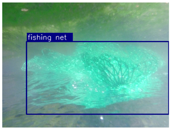
Figure 1.
For example, this plot shows the net detection results of YOLOv5. See that a bounding box is generated on the image of an underwater net. The center of a bounding box indicates the bearing angle of a net, with respect to the robot’s camera.
There are many papers on developing collision evasion controls [22,23,24,25]. In [26], an obstacle avoidance study of a wave glider in a 2D marine environment was conducted. Considering 2D environments, Artificial Potential Field (APF) has been widely used for avoid collision between a robot and obstacles [26,27]. APF is generated by the addition of the attraction potential field (generated by the goal) and the repulsive potential field (generated by obstacles). Velocity Obstacle (VO) methods can be utilized for collision evasion with moving obstacles [22,24,28,29,30,31]. References [31,32,33] considered collision avoidance in three-dimensional environments.
The collision avoidance methods in the previous paragraph provide the safe motion of a robot, in the case where an obstacle is detected by the robot’s sensor. Moreover, these collision avoidance methods assume that the distance between the robot and an obstacle can be accurately measured. To the best of our knowledge, collision avoidance methods in the literature assumed that the distance between the robot and an obstacle can be accurately measured. This implies that the collision avoidance controls in the literature require that the robot has range sensors.
Our paper considers passive camera sensors that do not provide the distance information between the robot and a detected net. Camera sensors only measure the bearing angle of a net, with respect to the robot’s camera pose. As far as we know, our paper is novel in developing reactive control laws for avoiding collisions based on the net’s bearing angle, which is computed based on the net’s bounding box.
In practice, the detection of underwater nets using camera images is not trivial. For instance, there may be trailing wires that extend from a net, and the wires can entangle the robot before the robot detects the net. Moreover, light, viewpoint and sea floor condition can decrease the net detection probability in practice. Light propagation in underwater environments suffers from turbidity, absorption and scattering, which strongly affect visual perception [21]. Thus, whenever a fishing net is detected using camera image, it is desirable to move away from the detected net abruptly.
In the proposed net avoidance controls, the robot moves away from a detected net whenever it detects a net. Here, the image bounding box position of the net is used to derive the bearing angle of the net with respect to the robot’s camera. Then, the bearing angle is used to make the robot move away from the detected net.
See Figure 2 for an example of the bearing angle of the net with respect to the robot’s camera. In this figure, b denotes the bearing angle of the net with respect to the robot’s camera. The bold plaid indicates the net in the camera image. A bounding box containing the detected net is plotted with a dotted rectangle. In order to move away from the detected net, the spherical robot at moves in the dashed arrow direction.
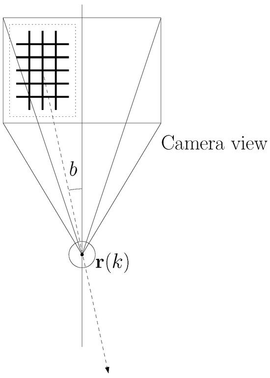
Figure 2.
An example of the bearing angle of the net with respect to the robot’s camera. Here, b denotes the bearing angle of the net with respect to the robot’s camera. The bold plaid indicates the net in the camera image. A bounding box containing the detected net is plotted with a dotted rectangle. In order to move away from the detected net, the spherical robot at moves in the dashed arrow direction.
After the robot moves backward for a certain distance, the robot makes a large circular turn to approach the goal, while avoiding the net. A large circular turn is used, since moving close to a net is dangerous for the robot. The proposed net avoidance controls are simple, and are suitable for real-time embedded system applications.
To the best of our knowledge, our article is novel in addressing reactive control laws for approaching the goal, while avoiding nets detected using passive cameras. The effectiveness of our net avoidance controls is verified using computer simulations.
2. Net Avoidance Controls
Before presenting our net avoidance controls, we address the motion model of the robot. This paper considers a spherical underwater robot as our platform [34,35,36,37]. A spherical robot may move slower than a torpedo-shaped underwater vehicle. However, due to the high water pressure resistance of spherical objects, a spherical robot can perform rotational motions with a 0 degree turn radius.
Let T denote a sampling interval in discrete time systems. Let r denote the robot moving in 2D environments. We assume that the robot can localize itself and can access the goal’s location. For instance, Visual-Inertial Simultaneous Localization And Mapping (VI-SLAM) [38,39] or monocular SLAM [40,41,42] can be applied for robot localization in real-time.
Let denote the 2D position of the goal in the inertial reference frame. Let denote the 2D position of the robot at time step k in the inertial reference frame. Let denote the velocity vector of the robot at time step k. The motion dynamics of the robot r are given as
By changing the robot’s thruster’s rotation direction, the robot can change its velocity vector at time step k. The motion model in (1) has been widely applied in the literature on robot controls [43,44,45,46,47,48,49,50].
The references [34,35,36] showed that by adopting vectored water-jets, a spherical underwater robot can maneuver freely in any direction. Since a spherical robot is highly maneuverable, the simple process model in (1) is feasible.
In order to move towards the goal, the robot sets its velocity vector as
where S denotes the speed of the robot.
While the robot moves towards its goal, it may detect a net using its camera. We can apply deep neural networks, such as YOLOv5 [19], for underwater net detection. Note that underwater net detection under camera measurements is not our novel contribution.
For enhancing the underwater net detection ability, we can apply various image enhancement operations [51], as well as image data augmentation techniques [52]. However, underwater net detection using camera sensors is not trivial in practice. Thus, whenever a net is detected using the robot’s camera, the robot moves away from the detected net abruptly. For moving away from the detected net, the robot uses the bearing angle of the net with respect to the robot’s camera.
Recall that Figure 2 depicts the bearing angle of the net with respect to the robot’s camera. In this figure, b denotes the bearing angle of the net with respect to the robot’s camera. A bold plaid indicates the net in the camera image. A bounding box containing the detected net is plotted with a dotted rectangle. In order to move away from the detected net, the spherical robot at moves in the dashed arrow direction.
After the robot moves backward for a certain distance, the robot makes a large circular turn to approach the goal, while avoiding the net. A large circular turn is desirable, since moving close to a net is dangerous for the robot.
Algorithm 1 presents the proposed net avoidance controls. In this algorithm, indicates the rotation direction of the robot, while circling around a detected net. Both directions of movement can avoid obstacles. However, considering a net which is partially observable by the robot, the robot cannot access which maneuver leads to net avoidance. In Algorithm 1, we set initially.
In Algorithm 1, the robot stores the recent trajectory of the robot. Let denote a tuning parameter determining the storage window size. At each time step k, the stored trajectory list is given as
Here, is called the reset point.
We say that the robot is stuck, in the case where every robot position in
is inside a circle with radius . Here, is a tuning parameter determining the stuck situation. As decreases, the robot is stuck in a smaller space.
Once the robot is stuck, it moves towards the reset point until reaching the reset point. As the robot reaches the reset point, it moves towards the goal. Suppose that the robot has been using as its maneuver strategy before it enters the stuck situation. In order to find a way to get out of the stuck situation, the robot changes its maneuver strategy using (). In this way, as the robot detects a net during its maneuver, it circles around the detected net in the reverse direction. The effect of this reverse maneuver strategy is presented in Section 3.2.3.
In Algorithm 1, the robot moves towards the goal by setting its velocity vector as (2). In Algorithms 1 and 2, is performed whenever the robot detects a net during its maneuver.
| Algorithm 1 Net avoidance controls |
|
| Algorithm 2 |
|
In Algorithm 2, the robot moves away from a detected net for D distance units. Here, D is a tuning constant, presenting the maximum sensing range of the robot. In simulations, we check the effect of changing D.
Let denote the 2D position of the net detected by the robot. Note that the robot cannot access using its camera measurements. The robot can only access the unit vector using the net’s bounding box in the camera image. In Figure 2, a dashed arrow indicates the direction associated to . Note that the relative distance cannot be provided using passive camera sensors.
By reversing the robot’s thruster’s rotation direction, the robot can move backwards. In order to move away from , the robot sets its velocity vector as
The robot moves away from a detected net for D distance units, by setting its velocity vector as (5) for s.
In Algorithm 2, the robot moves along a half circle with radius D. Before addressing the robot’s velocity vector for this circling maneuver, we define the rotation matrix as
Here, indicates the rotation matrix of in radians. Let denote the robot’s 2D location at the moment when the robot begins moving away from a detected net for D distance units. The robot can access , since the robot can localize itself using various localization methods, such as VI-SLAM [38,39] or monocular SLAM [40,41,42]. By setting the robot’s velocity vector as
the robot moves along a circle with radius D. The robot moves along a half circle with radius D, by setting its velocity vector as (7) for s.
In (7), indicates the rotation direction of the robot, while moving along a half circle with radius D. Here, implies that the robot moves along a half circle with radius D in the counter-clockwise direction. In addition, implies that the robot moves along a half circle with radius D in the clockwise direction. In Algorithm 2, is reversed only in the case where the robot is stuck. Here, is reversed to make the robot remove itself from the stuck situation.
Figure 3 shows an example of net avoidance controls. A red dashed line segment indicates a net. The goal is marked with a cross. The top subplot shows the case where the robot detects the net, while moving towards the goal. The below subplot shows the case where the robot moves away from the detected net for D distance units, followed by moving along a half circle with radius D. Then, the robot can move towards the goal without being entangled by nets.
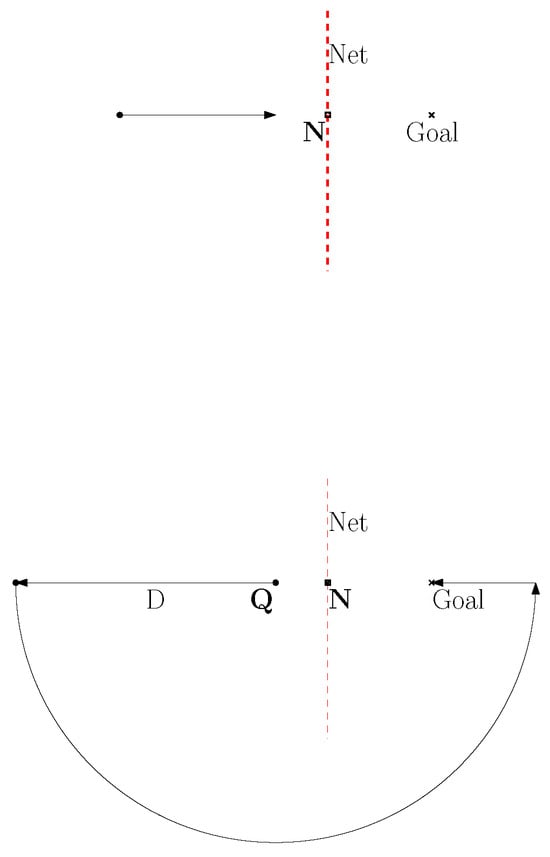
Figure 3.
Example of net avoidance controls. A red dashed line segment indicates a net. The goal is marked with a cross. The top subplot shows the case where the robot detects the net, while moving towards the goal. The below subplot shows the case where the robot moves away from the detected net for D distance units, followed by moving along a half circle with radius D. Then, the robot can move towards the goal without being entangled by nets.
Discussion
We acknowledge that the proposed net avoidance controls are not optimal, since the robot does not move along a shortest path to the goal. However, we argue that finding an optimal path is not possible, since the robot moves in unknown underwater environments. An optimal path can be generated only when we have a priori knowledge on obstacle environments.
Moreover, the robot cannot detect the accurate position of underwater nets using camera sensors with limited field of view. The robot can only measure the bearing angle of the detected net, with respect to its camera. Note that our collision avoidance control laws are based on the net’s bearing direction, which is computed based on the net’s bounding box. As far as we know, our paper is unique in addressing how to reach the goal, while avoiding collision with nets detected using passive cameras.
3. MATLAB Simulations
3.1. Net Detection Experiments
We show that deep neural networks can be trained to detect a fishing net. We applied YOLOv5 [19] for underwater net detection. Note that underwater net detection under camera measurements is not our novel contribution. For net detection, we can apply other types of neural networks, such as Fast R-CNN [15], Faster R-CNN [16], or Mask R-CNN [17].
In order to generate datasets related to underwater nets, we do experiments in the stream. In YOLOv5 [19], the neural network model is trained using 700 fishing net images with a validation set of 1000 images. The models are evaluated on a testing set of size 1000 images. Each image size is . The neural network is optimized using stochastic gradient descent, which has a learning rate of . Another parameter is weight decay, which is set to with momentum. The batch size and epochs are 256 and 600, respectively. We used GPU (Nvidia Tesla V100 32GB) for our experiments.
Using YOLOv5 [19], we reached 0.95 mean Average Precision (mAP), when the threshold of IOU is set to 0.5. This implies that the proposed net detection can be applied in practice. We achieved 33 frames per second (FPS); thus, real-time net detection is feasible. Figure 1 shows the detection results of YOLOv5, which is applied to experiments in the stream.
3.2. Net Avoidance Simulations
Using MATLAB simulations, we verify the effectiveness of the proposed net avoidance controls (Algorithm 1). To the best of our knowledge, collision avoidance methods in the literature assumed that the distance between the robot and an obstacle can be accurately measured. This implies that the collision avoidance controls in the literature require that the robot has range sensors. However, in our paper, the robot only detects the bearing angle of a net, with respect to the robot’s passive camera.
The goal is located at the origin. The motion dynamics of the robot are given in (1), and the robot’s speed is m/s. Recall we consider a spherical underwater robot as our platform [34,35,36,37]. Thanks to the high water pressure resistance of spherical objects, a spherical robot can perform rotational motions with a 0 degree turn radius. By adopting vectored water-jets, a spherical underwater robot can maneuver freely in any direction [34,35,36].
We assume that the robot is entangled by a net, in the case where the distance from the net and the robot is less than 0.1 m. In (3) and (4), we use time steps and (m). These parameters ( and ) are used in all simulations.
In practice, the robot may not detect a net, even in the case where the net is within the camera sensing range. Light, viewpoint, and sea floor condition can decrease the net detection probability in practice. We assume that the robot detects a net with probability , as long as the relative distance between the robot and a point in the net is less than D. This implies that a net is found with probability , as long as the net is within D distance from the robot. We use (m) and .
We ran 30 Monte-Carlo (MC) simulations to verify the outperformance of Algorithm 1 rigorously. In every MC simulation, we randomly set the initial location of the robot in the box with size in meters. Per each MC simulation, the robot approached the goal, while avoiding collision with detected nets. We randomly changed the initial location, since this random initialization provides robust performance analysis of the proposed algorithm. If we fix the initial robot location in all MC simulations, then the trajectory of the robot does not change at every MC simulation.
As specific quantitative metrics to evaluate the effectiveness of the net avoidance control strategy, we use the average travel distance in every MC simulation and the computation time for all MC simulations. For convenience, denotes the average travel distance of a robot in every MC simulation. Let denote the computation time of all MC simulations. It is desirable that both and are as short as possible.
Considering the case where (m) and , Figure 4 shows the trajectory of the robot for 30 MC simulations. Whenever the robot is entangled by a net, the associated MC simulation ends. In Figure 4, the initial position of the robot is marked with a red circle. In each MC simulation, the trajectory of the robot at every 10 s is marked with asterisks of distinct colors. Blue line segments indicate underwater nets. Figure 4 shows that the robot reaches the goal in all MC simulations, while avoiding collision with nets.
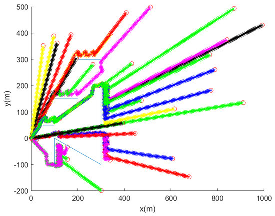
Figure 4.
We set (m) and . This plot shows the trajectory of the robot for 30 MC simulations. Per each MC simulation, the initial position of the robot is marked with a red circle. In each MC simulation, the trajectory of the robot at every 10 s is marked with asterisks of distinct colors. Blue line segments indicate underwater nets. See that the robot reaches the goal, while avoiding collision with underwater nets.
From Figure 4 where (m) and , we obtain as 699 m. is 16 s. The proposed net avoidance controls are simple, and are suitable for real-time embedded system applications.
3.2.1. The Effect of Changing the Maximum Sensing Range D
In clear water, the maximum sensing range D can be large. But, in dark and dirty water, D can be small. We further present the effect of changing D. We set (m) and .
Considering the case where (m) and , Figure 5 shows the trajectory of the robot for 30 MC simulations. The initial position of the robot is marked with a red circle. In each MC simulation, the trajectory of the robot at every 10 s is marked with asterisks of distinct colors. Blue line segments indicate underwater nets. Figure 5 shows that the robot reaches the goal, while avoiding collision with nets.
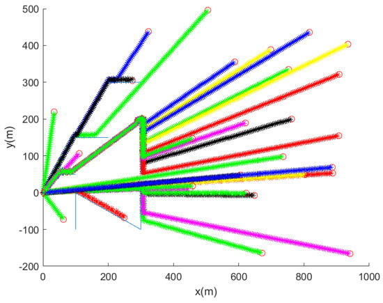
Figure 5.
We set (m) and . This plot shows the trajectory of the robot for 30 MC simulations. Per each MC simulation, the initial position of the robot is marked with a red circle. In each MC simulation, the trajectory of the robot at every 10 s is marked with asterisks of distinct colors. Blue line segments indicate underwater nets. See that the robot reaches the goal, while avoiding collision with underwater nets.
From Figure 5 where (m) and , we obtain as 746 m, and is 23 s. Recall that as we use (m) and , we obtain as 699 m (Figure 4), and is 16 s. See that as D decreases to 5 (m), both and increase. This implies that the robot can reach its goal fast, as the robot is in clear water, compared to the case where the robot is in dark and dirty water.
3.2.2. The Effect of Changing the Detection Probability
We next check the effect of changing the detection probability . In dark, dirty, and cluttered underwater environments, can be small. We set , while setting m.
As we set (m) and , Figure 6 shows the trajectory of the robot for 30 MC simulations. The initial location of the robot is marked with a red circle. In each MC simulation, the trajectory of the robot at every 10 s is marked with asterisks of distinct colors. Blue line segments indicate underwater nets. Despite the setting of low , the robot reaches the goal in all MC simulations, while avoiding collision with nets.
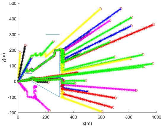
Figure 6.
We set , while setting m. This plot shows the trajectory of the robot for 30 MC simulations. Per each MC simulation, the initial position of the robot is marked with a red circle. In each MC simulation, the trajectory of the robot at every 10 s is marked with asterisks of distinct colors. Blue line segments indicate underwater nets. See that the robot reaches the goal, while avoiding collision with underwater nets.
3.2.3. The Effect of Using the Strategy for Getting Out of the Stuck Situation
Once the robot is stuck, it moves towards the reset point until reaching the reset point. Then, the robot changes its maneuver strategy () for getting out of the stuck situation. We next verify the effect of using this strategy for getting out of the stuck situation.
Suppose that one does not apply the strategy for getting out of the stuck situation. We do not apply this strategy by setting . Recall that the robot is stuck, in the case where every robot position in (4) is inside a circle with radius .
Figure 7 shows the trajectory of the robot, as we do not apply the strategy for getting out of the stuck situation. See that the robot cannot get out of the stuck situation. In Figure 7, we set , while setting m.
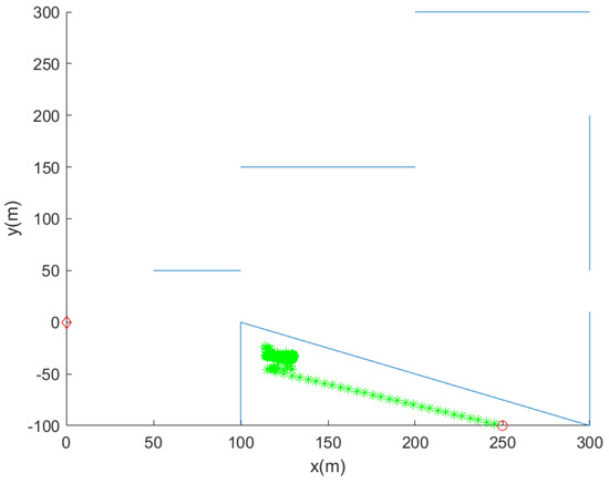
Figure 7.
One does not apply the strategy for getting out of the stuck situation. We do not apply this strategy by setting . We further set , while setting m. The initial position of the robot is marked with a red circle. The trajectory of the robot at every 10 s is marked with asterisks of distinct colors. Blue line segments indicate underwater nets. See that the robot cannot get out of the stuck situation.
Considering the scenario in Figure 7 ( (m) and ), Figure 8 shows the trajectory of the robot, as we apply the strategy for getting out of the stuck situation. We apply this strategy by setting (m). See that the robot reaches the goal after getting out of the stuck situation.
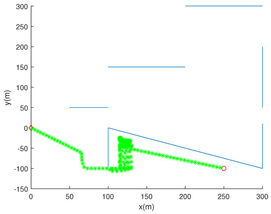
Figure 8.
One applies the strategy for getting out of the stuck situation. We apply this strategy by setting (m). We also set , while setting m. The initial position of the robot is marked with a red circle. The trajectory of the robot at every 10 s is marked with asterisks of distinct colors. Blue line segments indicate underwater nets. See that the robot reaches the goal after getting out of the stuck situation.
4. Conclusions
This paper proposes camera-based fishing net avoidance controls. Passive camera sensors do not provide the distance information between the robot and a net. Camera sensors generate the bearing angle of a net, with respect to the robot’s camera pose. Whenever a net is detected by the robot’s camera, the robot avoids the detected net by moving away from the net. Here, the bounding box of the net image is used to make the robot move away from the net.
After the robot moves backwards for a while, it makes a large circular turn followed by heading towards its goal. A large circular turn is applied, since moving close to a net is dangerous for the robot. To the best of our knowledge, our article is novel in addressing reactive control laws for approaching the goal, while avoiding nets detected using cameras.
In practice, we may have a partial information on the underwater workspace. For instance, we may have a priori information on underwater terrain environments. Based on partially known underwater environments, we can generate a shortest path from the start to the goal using various path planners, such as A-star or Dijkstra algorithms [53]. We then set waypoints along the shortest path. In order to make the robot move from one waypoint to the next one, we can use the proposed control laws. In other words, our control laws can be used to move from one waypoint to the next one, while avoiding collision with underwater nets.
The effectiveness of the proposed net avoidance controls is verified using experiments and simulations. The proposed net avoidance controls are simple, and are suitable for real-time embedded system applications. In the future, we will verify the proposed net avoidance controls by doing experiments with real underwater robots. Also, in the future, we will extend the proposed controls to multi-robot systems [54,55,56], so that a group of multiple underwater robots can move towards a goal while avoiding underwater nets.
Funding
This work was supported by the National Research Foundation of Korea (NRF) grant funded by the Korea government (MSIT) (Grant Number: 2022R1A2C1091682). This research was supported by the faculty research fund of Sejong university in 2023.
Institutional Review Board Statement
Not applicable.
Informed Consent Statement
Not applicable.
Data Availability Statement
Data are contained within the article.
Conflicts of Interest
The authors declare no conflicts of interest.
References
- Sahoo, A.; Dwivedy, S.K.; Robi, P. Advancements in the field of autonomous underwater vehicle. Ocean. Eng. 2019, 181, 145–160. [Google Scholar] [CrossRef]
- Zhang, X.; Fan, Y.; Liu, H.; Zhang, Y.; Sha, Q. Design and Implementation of Autonomous Underwater Vehicle Simulation System Based on MOOS and Unreal Engine. Electronics 2023, 12, 3107. [Google Scholar] [CrossRef]
- Ribas, D.; Ridao, P.; Domingo Tardos, J.; Neira, J. Underwater SLAM in a marina environment. In Proceedings of the 2007 IEEE/RSJ International Conference on Intelligent Robots and Systems, San Diego, CA, USA, 29 October–2 November 2007; pp. 1455–1460. [Google Scholar]
- Allotta, B.; Costanzi, R.; Fanelli, F.; Monni, N.; Paolucci, L.; Ridolfi, A. Sea currents estimation during AUV navigation using Unscented Kalman Filter. IFAC PapersOnLine 2017, 50, 13668–13673. [Google Scholar] [CrossRef]
- Kim, J. Underwater surface scan utilizing an unmanned underwater vehicle with sampled range information. Ocean. Eng. 2020, 207, 107345. [Google Scholar] [CrossRef]
- Machado Jorge, V.A.; de Cerqueira Gava, P.D.; Belchior de França Silva, J.R.; Mancilha, T.M.; Vieira, W.; Adabo, G.J.; Nascimento, C.L. Analytical Approach to Sampling Estimation of Underwater Tunnels Using Mechanical Profiling Sonars. Sensors 2021, 21, 1900. [Google Scholar] [CrossRef] [PubMed]
- Kim, J. Underwater guidance of distributed autonomous underwater vehicles using one leader. Asian J. Control 2023, 25, 2641–2654. [Google Scholar] [CrossRef]
- Goheen, K.; Jefferys, E. The application of alternative modelling techniques to ROV dynamics. In Proceedings of the IEEE International Conference on Robotics and Automation, Cincinnati, OH, USA, 13–18 May 1990; Volume 2, pp. 1302–1309. [Google Scholar]
- Mai, C.; Liniger, J.; Jensen, A.L.; Sørensen, H.; Pedersen, S. Experimental Investigation of Non-contact 3D Sensors for Marine-growth Cleaning Operations. In Proceedings of the 2022 IEEE 5th International Conference on Image Processing Applications and Systems (IPAS), Genova, Italy, 5–7 December 2022; Volume 5, pp. 1–6. [Google Scholar]
- O’Byrne, M.; Schoefs, F.; Pakrashi, V.; Ghosh, B. An underwater lighting and turbidity image repository for analysing the performance of image-based non-destructive techniques. Struct. Infrastruct. Eng. 2018, 14, 104–123. [Google Scholar] [CrossRef]
- Chen, Z.; Zhang, Z.; Dai, F.; Bu, Y.; Wang, H. Monocular vision-based underwater object detection. Sensors 2017, 17, 1784. [Google Scholar] [CrossRef]
- Foresti, G.L.; Gentili, S. A vision based system for object detection in underwater images. Int. J. Pattern Recognit. Artif. Intell. 2000, 14, 167–188. [Google Scholar] [CrossRef]
- Rizzini, D.L.; Kallasi, F.; Oleari, F.; Caselli, S. Investigation of vision-based underwater object detection with multiple datasets. Int. J. Adv. Robot. Syst. 2015, 12, 77. [Google Scholar] [CrossRef]
- Hovem, J. Underwater acoustics: Propagation, devices and systems. J. Electroceram. 2007, 19, 339–347. [Google Scholar] [CrossRef]
- Girshick, R. Fast r-cnn. In Proceedings of the IEEE International Conference on Computer Vision, Santiago, Chile, 7–13 December 2015; pp. 1440–1448. [Google Scholar]
- Ren, S.; He, K.; Girshick, R.; Sun, J. Faster r-cnn: Towards real-time object detection with region proposal networks. In Advances in Neural Information Processing Systems; Springer: Berlin/Heidelberg, Germany, 2015; Volume 28. [Google Scholar]
- He, K.; Gkioxari, G.; Dollár, P.; Girshick, R. Mask r-cnn. In Proceedings of the IEEE International Conference on Computer Vision, Venice, Italy, 22–29 October 2017; pp. 2961–2969. [Google Scholar]
- Redmon, J.; Farhadi, A. Yolov3: An incremental improvement. arXiv 2018, arXiv:1804.02767. [Google Scholar]
- Karthi, M.; Muthulakshmi, V.; Priscilla, R.; Praveen, P.; Vanisri, K. Evolution of YOLO-V5 Algorithm for Object Detection: Automated Detection of Library Books and Performace validation of Dataset. In Proceedings of the 2021 International Conference on Innovative Computing, Intelligent Communication and Smart Electrical Systems (ICSES), Chennai, India, 24–25 September 2021; pp. 1–6. [Google Scholar]
- Wang, C.Y.; Bochkovskiy, A.; Liao, H.Y.M. YOLOv7: Trainable bag-of-freebies sets new state-of-the-art for real-time object detectors. arXiv 2022, arXiv:2207.02696. [Google Scholar]
- Sørensen, F.F.; Mai, C.; Olsen, O.M.; Liniger, J.; Pedersen, S. Commercial Optical and Acoustic Sensor Performances under Varying Turbidity, Illumination, and Target Distances. Sensors 2023, 23, 6575. [Google Scholar] [CrossRef] [PubMed]
- van den Berg, J.; Guy, S.J.; Ming Lin and, D.M. Reciprocal n-Body Collision Avoidance. Robot. Res. Springer Tracts Adv. Robot. 2011, 70, 3–19. [Google Scholar]
- Kosecka, J.; Tomlin, C.; Pappas, G.; Sastry, S. Generation of conflict resolution maneuvers for air traffic management. In Proceedings of the International Conference of Intelligent Robotic Systems, Grenoble, France, 7–11 September 1997; pp. 1598–1603. [Google Scholar]
- Chakravarthy, A.; Ghose, D. Obstacle avoidance in a dynamic environment: A collision cone approach. IEEE Trans. Syst. Man Cybern. 1998, 28, 562–574. [Google Scholar] [CrossRef]
- Lalish, E.; Morgansen, K. Distributed reactive collision avoidance. Auton. Robot. 2012, 32, 207–226. [Google Scholar] [CrossRef]
- Wang, D.; Wang, P.; Zhang, X.; Guo, X.; Shu, Y.; Tian, X. An obstacle avoidance strategy for the wave glider based on the improved artificial potential field and collision prediction model. Ocean. Eng. 2020, 206, 107356. [Google Scholar] [CrossRef]
- Mohammad, S.; Rostami, H.; Sangaiah, A.K.; Wang, J.; Liu, X. Obstacle avoidance of mobile robots using modified artificial potential field algorithm. EURASIP J. Wirel. Commun. Netw. 2019, 70, 1–19. [Google Scholar]
- Lalish, E. Distributed Reactive Collision Avoidance; University of Washington: Washington, DC, USA, 2009. [Google Scholar]
- Sunkara, V.; Chakravarthy, A. Collision avoidance laws for objects with arbitrary shapes. In Proceedings of the 2016 IEEE 55th Conference on Decision and Control (CDC), Las Vegas, NV, USA, 12–14 December 2016; pp. 5158–5164. [Google Scholar]
- Leonard, J.; Savvaris, A.; Tsourdos, A. Distributed reactive collision avoidance for a swarm of quadrotors. Proc. Inst. Mech. Eng. Part J. Aerosp. Eng. 2017, 231, 1035–1055. [Google Scholar] [CrossRef]
- Kim, J. Reactive Control for Collision Evasion with Extended Obstacles. Sensors 2022, 22, 5478. [Google Scholar] [CrossRef] [PubMed]
- Zheng, Z.; Bewley, T.R.; Kuester, F. Point Cloud-Based Target-Oriented 3D Path Planning for UAVs. In Proceedings of the 2020 International Conference on Unmanned Aircraft Systems (ICUAS), Athens, Greece, 1–4 September 2020; pp. 790–798. [Google Scholar]
- Roelofsen, S.; Martinoli, A.; Gillet, D. 3D collision avoidance algorithm for Unmanned Aerial Vehicles with limited field of view constraints. In Proceedings of the 2016 IEEE 55th Conference on Decision and Control (CDC), Las Vegas, NV, USA, 12–14 December 2016; pp. 2555–2560. [Google Scholar]
- Gu, S.; Guo, S.; Zheng, L. A highly stable and efficient spherical underwater robot with hybrid propulsion devices. Auton. Robot 2020, 44, 759–771. [Google Scholar] [CrossRef]
- Yue, C.; Guo, S.; Shi, L. Hydrodynamic Analysis of the Spherical Underwater Robot SUR-II. Int. J. Adv. Robot. Syst. 2013, 10, 247. [Google Scholar] [CrossRef]
- Li, C.; Guo, S.; Guo, J. Tracking Control in Presence of Obstacles and Uncertainties for Bioinspired Spherical Underwater Robots. J. Bionic Eng. 2023, 20, 323–337. [Google Scholar] [CrossRef]
- Kim, J. Leader-Based Flocking of Multiple Swarm Robots in Underwater Environments. Sensors 2023, 23, 5305. [Google Scholar] [CrossRef] [PubMed]
- Chen, C.; Zhu, H.; Li, M.; You, S. A Review of Visual-Inertial Simultaneous Localization and Mapping from Filtering-Based and Optimization-Based Perspectives. Robotics 2018, 7, 45. [Google Scholar] [CrossRef]
- Lynen, S.; Zeisl, B.; Aiger, D.; Bosse, M.; Hesch, J.; Pollefeys, M.; Siegwart, R.; Sattler, T. Large-scale, real-time visual–inertial localization revisited. Int. J. Robot. Res. 2020, 39, 1061–1084. [Google Scholar] [CrossRef]
- Strasdat, H.; Montiel, J.M.M.; Davison, A.J. Real-time monocular SLAM: Why filter? In Proceedings of the 2010 IEEE International Conference on Robotics and Automation, Anchorage, AK, USA, 3–7 May 2010; pp. 2657–2664. [Google Scholar]
- Eade, E.; Drummond, T. Scalable Monocular SLAM. In Proceedings of the 2006 IEEE Computer Society Conference on Computer Vision and Pattern Recognition (CVPR’06), New York, NY, USA, 17–22 June 2006; Volume 1, pp. 469–476. [Google Scholar]
- Mur-Artal, R.; Montiel, J.M.M.; Tardós, J.D. ORB-SLAM: A Versatile and Accurate Monocular SLAM System. IEEE Trans. Robot. 2015, 31, 1147–1163. [Google Scholar] [CrossRef]
- Ji, M.; Egerstedt, M. Distributed Coordination Control of Multi-Agent Systems While Preserving Connectedness. IEEE Trans. Robot. 2007, 23, 693–703. [Google Scholar] [CrossRef]
- Garcia de Marina, H.; Cao, M.; Jayawardhana, B. Controlling Rigid Formations of Mobile Agents Under Inconsistent Measurements. IEEE Trans. Robot. 2015, 31, 31–39. [Google Scholar] [CrossRef]
- Krick, L.; Broucke, M.E.; Francis, B.A. Stabilization of infinitesimally rigid formations of multi-robot networks. Int. J. Control 2009, 82, 423–439. [Google Scholar] [CrossRef]
- Kim, J.; Kim, S. Motion control of multiple autonomous ships to approach a target without being detected. Int. J. Adv. Robot. Syst. 2018, 15, 1729881418763184. [Google Scholar] [CrossRef]
- Luo, S.; Kim, J.; Parasuraman, R.; Bae, J.H.; Matson, E.T.; Min, B.C. Multi-robot rendezvous based on bearing-aided hierarchical tracking of network topology. Ad Hoc Netw. 2019, 86, 131–143. [Google Scholar] [CrossRef]
- Wu, W.; Zhang, F. A Speeding-Up and Slowing-Down Strategy for Distributed Source Seeking With Robustness Analysis. IEEE Trans. Control Netw. Syst. 2016, 3, 231–240. [Google Scholar] [CrossRef]
- Al-Abri, S.; Wu, W.; Zhang, F. A Gradient-Free Three-Dimensional Source Seeking Strategy With Robustness Analysis. IEEE Trans. Autom. Control 2019, 64, 3439–3446. [Google Scholar] [CrossRef]
- Kim, J. Three-dimensional multi-robot control to chase a target while not being observed. Int. J. Adv. Robot. Syst. 2019, 16, 1729881419829667. [Google Scholar] [CrossRef]
- Jian, M.; Liu, X.; Luo, H.; Lu, X.; Yu, H.; Dong, J. Underwater image processing and analysis: A review. Signal Process. Image Commun. 2021, 91, 116088. [Google Scholar] [CrossRef]
- Shorten, C.; Khoshgoftaar, T.M. A survey on image data augmentation for deep learning. J. Big Data 2019, 6, 1–48. [Google Scholar] [CrossRef]
- Lavalle, S.M. Planning Algorithms; Cambridge University Press: Cambridge, UK, 2006. [Google Scholar]
- Ikeda, T.; Mita, T.; Yamakita, M. Formation Control of Autonomous Underwater Vehicles. IFAC Proc. Vol. 2005, 38, 666–671. [Google Scholar] [CrossRef]
- Cui, R.; Xu, D.; Yan, W. Formation Control of Autonomous Underwater Vehicles under Fixed Topology. In Proceedings of the 2007 IEEE International Conference on Control and Automation, Guangzhou, China, 30 May–1 June 2007; pp. 2913–2918. [Google Scholar]
- Li, L.; Li, Y.; Zhang, Y.; Xu, G.; Zeng, J.; Feng, X. Formation Control of Multiple Autonomous Underwater Vehicles under Communication Delay, Packet Discreteness and Dropout. J. Mar. Sci. Eng. 2022, 10, 920. [Google Scholar] [CrossRef]
Disclaimer/Publisher’s Note: The statements, opinions and data contained in all publications are solely those of the individual author(s) and contributor(s) and not of MDPI and/or the editor(s). MDPI and/or the editor(s) disclaim responsibility for any injury to people or property resulting from any ideas, methods, instructions or products referred to in the content. |
© 2024 by the author. Licensee MDPI, Basel, Switzerland. This article is an open access article distributed under the terms and conditions of the Creative Commons Attribution (CC BY) license (https://creativecommons.org/licenses/by/4.0/).