
An Intelligent Ball Bearing Fault Diagnosis System Using Enhanced Rotational Characteristics on Spectrogram

Abstract
1. Introduction
- The proposed system extracts the fault features of ball bearings that are related to rotational frequency. This method does not require a high sampling rate for the accelerometer when collecting vibration signals.
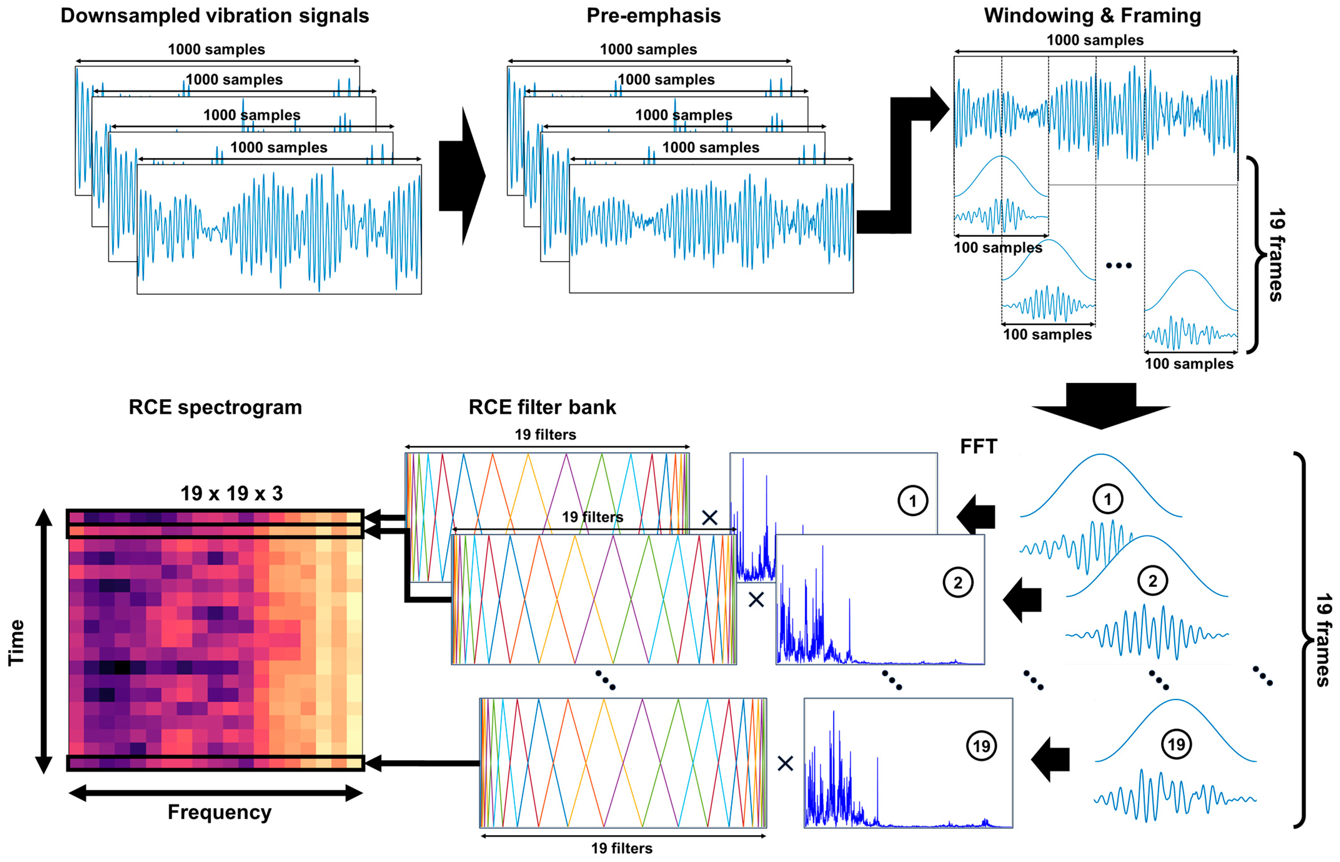
- Compared to existing studies that use MFCCs to extract the features of vibration signals, the RCE spectrogram process analyzes a narrow frequency band. This requires fewer resources than existing feature extraction methods. In addition, the optimized CNN architecture for fault classification has lower complexity than existing CNN architectures.
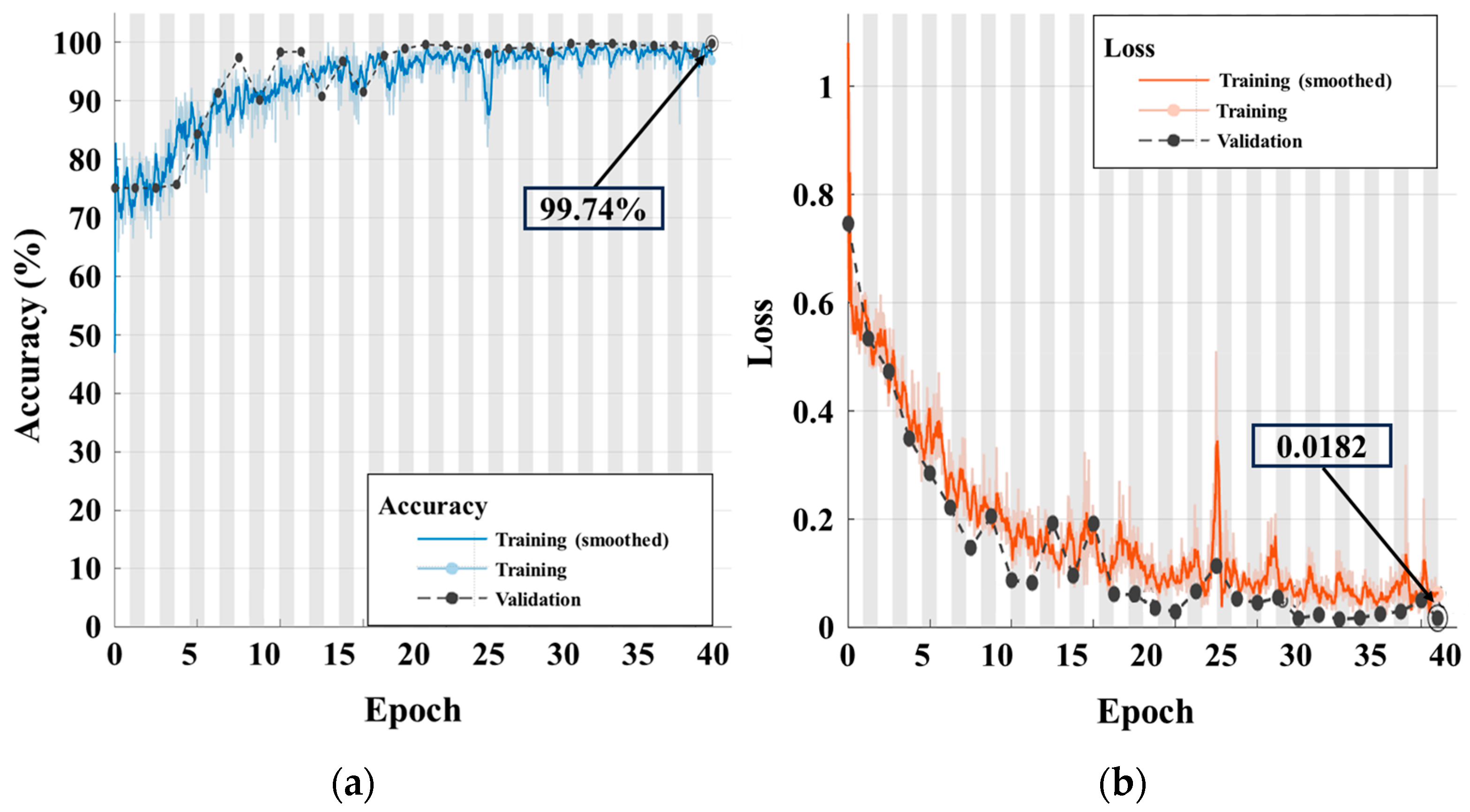
- The Case Western Reserve University (CWRU) dataset was used to evaluate the ball bearing fault diagnosis. The experimental results indicated that the proposed method classified ball bearing faults with an accuracy of 0.9974. This satisfies the conditions for a ball bearing fault diagnosis system.
2. Background Knowledge
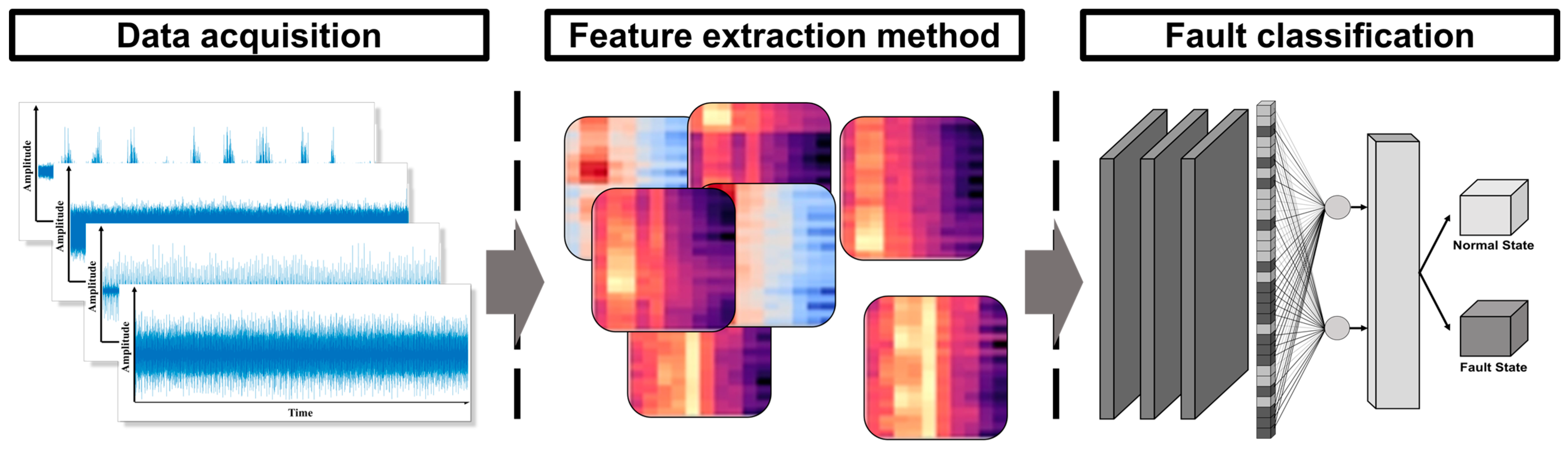
3. Proposed Ball Bearing Fault Diagnosis System
3.1. Feature Extraction Method
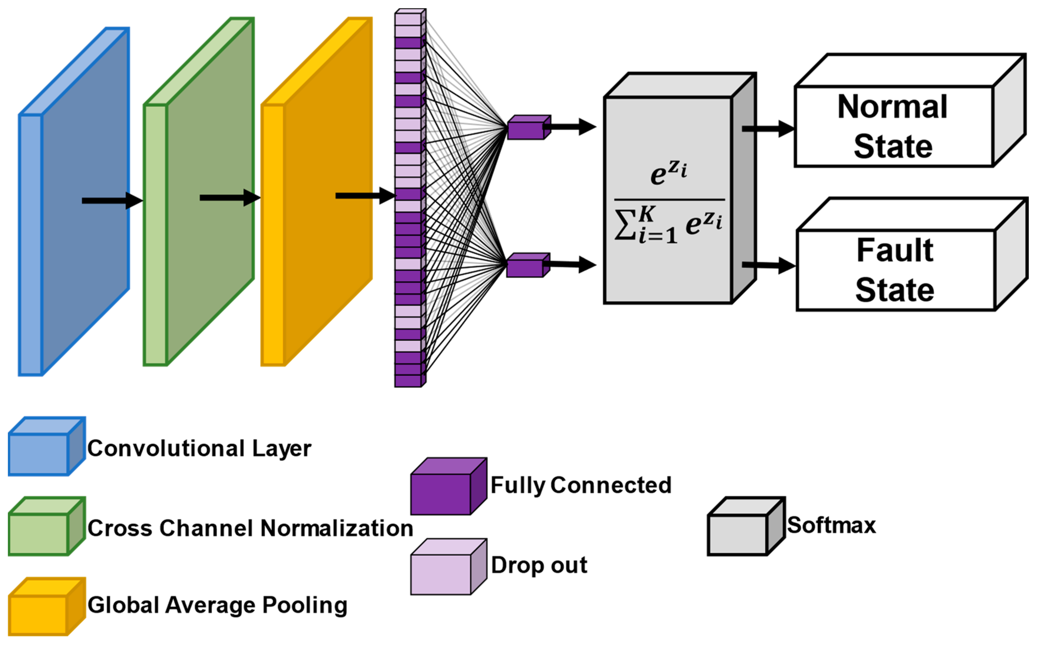
3.2. Fault Classification
4. Experiment
4.1. Experimental Setup and Dataset Description
4.2. Evaluation Details
4.3. Analysis Result
4.4. Comparison of the Results with Other Methods
5. Conclusions
Author Contributions
Funding
Institutional Review Board Statement
Informed Consent Statement
Data Availability Statement
Conflicts of Interest
References
- Grebenik, J.; Zhang, Y.; Bingham, C.; Srivastava, S. Roller Element Bearing Acoustic Fault Detection Using Smartphone and Consumer Microphones Comparing with Vibration Techniques. In Proceedings of the 17th International Conference on Mechatronics—Mechatronika (ME), Prague, Czech Republic, 7–9 December 2016; pp. 1–7. [Google Scholar]
- Cerrada, M.; Sánchez, R.V.; Li, C.; Pacheco, F.; Cabrera, D.; de Oliveira, J.V.; Vásquez, R.E. A review on data-driven fault severity assessment in rolling bearings. Mech. Syst. Signal Process. 2018, 99, 169–196. [Google Scholar] [CrossRef]
- Abdenebi, R.; Fethi, D.; Abdelkrim, N.; Badis, D. Gearbox Fault Diagnosis Using the Short-Time Cepstral Features. In Proceedings of the 2022 2nd International Conference on Advanced Electrical Engineering, ICAEE 2022, Constantine, Algeria, 29–31 October 2022; pp. 1–7. [Google Scholar] [CrossRef]
- Wang, Y.; Markert, R.; Xiang, J.; Zheng, W. Research on variational mode decomposition and its application in detecting rub-impact fault of the rotor system. Mech. Syst. Signal Process. 2015, 60–61, 243–251. [Google Scholar] [CrossRef]
- Saravanan, N.; Cholairajan, S.; Ramachandran, K.I. Vibration-based fault diagnosis of spur bevel gear box using fuzzy technique. Expert Syst. Appl. 2009, 36, 3119–3135. [Google Scholar] [CrossRef]
- Kumar, A.; Vashishtha, G.; Gandhi, C.P.; Zhou, Y.; Glowacz, A.; Xiang, J. Novel Convolutional Neural Network (NCNN) for the Diagnosis of Bearing Defects in Rotary Machinery. IEEE Trans. Instrum. Meas. 2021, 70, 3510710. [Google Scholar] [CrossRef]
- Choudhary, A.; Mian, T.; Fatima, S. Convolutional neural network based bearing fault diagnosis of rotating machine using thermal images. Measurement 2021, 176, 109196. [Google Scholar] [CrossRef]
- Younus, A.M.D.; Yang, B. Intelligent fault diagnosis of rotating machinery using infrared thermal image. Expert Syst. Appl. 2012, 39, 2082–2091. [Google Scholar] [CrossRef]
- Janssens, O.; Schulz, R.; Slavkovikj, V.; Stockman, K.; Loccufier, M.; Van de Walle, R.; Van Hoecke, S. Thermal image based fault diagnosis for rotating machinery. Infrared Phys. Technol. 2015, 73, 78–87. [Google Scholar] [CrossRef]
- Liu, Q.; Lu, X.; He, Z.; Zhang, C.; Chen, W.S. Deep convolutional neural networks for thermal infrared object tracking. Knowl. Based Syst. 2017, 134, 189–198. [Google Scholar] [CrossRef]
- Glowacz, A. Fault diagnosis of single-phase induction motor based on acoustic signals. Mech. Syst. Signal Process. 2019, 117, 65–80. [Google Scholar] [CrossRef]
- Marin, F.B.; Solomon, C.; Marin, M. Bearing Failure Prediction Using Audio Signal Analysis Based on SVM Algorithms. In Proceedings of the IOP Conference Series: Materials Science and Engineering, Galati, Romania, 11–13 October 2018; IOP Publishing: Bristol, UK, 2019; p. 012012. [Google Scholar] [CrossRef]
- Nirwan, N.W.; Ramani, H.B. Condition monitoring and fault detection in roller bearing used in rolling mill by acoustic emission and vibration analysis. Mater. Today Proc. 2022, 51, 344–354. [Google Scholar] [CrossRef]
- Wang, J.; He, Q.; Kong, F. Adaptive Multiscale Noise Tuning Stochastic Resonance for Health Diagnosis of Rolling Element Bearings. IEEE Trans. Instrum. Meas. 2015, 64, 564–577. [Google Scholar] [CrossRef]
- Wu, S.; Gebraeel, N.; Lawley, M.A.; Yih, Y. A Neural Network Integrated Decision Support System for Condition-Based Optimal Predictive Maintenance Policy. IEEE Trans. Syst. Man Cybern. Part A Syst. Hum. 2007, 37, 226–236. [Google Scholar] [CrossRef]
- Zhou, Y.; Wang, H.; Wang, G.; Kumar, A.; Sun, W.; Xiang, J. Semi-Supervised Multiscale Permutation Entropy-Enhanced Contrastive Learning for Fault Diagnosis of Rotating Machinery. IEEE Trans. Instrum. Meas. 2023, 72, 3525610. [Google Scholar] [CrossRef]
- Chen, Z.; Cen, J.; Xiong, J. Rolling Bearing Fault Diagnosis Using Time-Frequency Analysis and Deep Transfer Convolutional Neural Network. IEEE Access 2020, 8, 150248–150261. [Google Scholar] [CrossRef]
- Chen, J.; Jiang, J.; Guo, X.; Tan, L. An Efficient CNN with Tunable Input-Size for Bearing Fault Diagnosis. Int. J. Comput. Intell. Syst. 2021, 14, 625–634. [Google Scholar] [CrossRef]
- Shan, S.; Liu, J.; Wu, S.; Shao, Y.; Li, H. A motor bearing fault voiceprint recognition method based on Mel-CNN model. Measurement 2023, 207, 112408. [Google Scholar] [CrossRef]
- Xia, M.; Li, T.; Xu, L.; Liu, L.; de Silva, C.W. Fault Diagnosis for Rotating Machinery Using Multiple Sensors and Convolutional Neural Networks. IEEE/ASME Trans. Mechatron. 2018, 23, 101–110. [Google Scholar] [CrossRef]
- Zhao, Y.; Zhang, N.; Zhang, Z.; Xu, X. Bearing Fault Diagnosis Based on Mel Frequency Cepstrum Coefficient and Deformable Space-Frequency Attention Network. IEEE Access 2023, 11, 34407–34420. [Google Scholar] [CrossRef]
- Choudakkanavar, G.; Mangai, J.A.; Bansal, M. MFCC based ensemble learning method for multiple fault diagnosis of roller bearing. Int. J. Inf. Technol. 2022, 14, 2741–2751. [Google Scholar] [CrossRef]
- Randall, R.B.; Antoni, J. Rolling element bearing diagnostics—A tutorial. Mech. Syst. Signal Process. 2011, 25, 485–520. [Google Scholar] [CrossRef]
- Akpudo, U.E.; Hur, J.W. A Cost-Efficient MFCC-Based Fault Detection and Isolation Technology for Electromagnetic Pumps. Electronics 2021, 10, 439. [Google Scholar] [CrossRef]
- Pham, M.T.; Kim, J.M.; Kim, C.H. Accurate bearing fault diagnosis under variable shaft speed using convolutional neural networks and vibration spectrogram. Appl. Sci. 2020, 10, 6385. [Google Scholar] [CrossRef]
- Zilong, Z.; Wei, Q. Intelligent Fault Diagnosis of Rolling Bearing Using One-Dimensional Multi-Scale Deep Convolutional Neural Network Based Health State Classification. In Proceedings of the 2018 IEEE 15th International Conference on Networking, Sensing and Control (ICNSC), Zhuhai, China, 27–29 March 2018; pp. 1–6. [Google Scholar] [CrossRef]
- Liu, R.; Meng, G.; Yang, B.; Sun, C.; Chen, X. Dislocated time series convolutional neural architecture: An intelligent fault diagnosis approach for electric machine. IEEE Trans. Ind. Inform. 2017, 13, 1310–1320. [Google Scholar] [CrossRef]
- Zhen, D.; Li, D.; Feng, G.; Zhang, H.; Gu, F. Rolling bearing fault diagnosis based on VMD reconstruction and DCS demodulation. Int. J. Hydromechatron. 2022, 5, 205–225. [Google Scholar] [CrossRef]
- Case Western Reserve University Bearing Dataset. Available online: https://engineering.case.edu/bearingdatacenter (accessed on 18 January 2023).
- Tandon, N.; Choudhury, A. A review of vibration and acoustic measurement methods for the detection of defects in rolling element bearings. Tribol. Int. 1999, 32, 469–480. [Google Scholar] [CrossRef]
- Tandon, N.; Nakra, B.C. Technical Article. Practical articles in shock and vibration technology: Vibration and Acoustic Monitoring Techniques for the Detection of Defects in Rolling Element Bearings—A Review. Shock Vib. Dig. 1992, 24, 3–11. [Google Scholar] [CrossRef]
- Jiang, Q.; Chang, F.; Sheng, B. Bearing fault classification based on convolutional neural network in noise environment. IEEE Access 2019, 7, 69795–69807. [Google Scholar] [CrossRef]
- Lu, S.; Lu, Z.; Zhang, Y.D. Pathological brain detection based on AlexNet and transfer learning. J. Comput. Sci. 2019, 30, 41–47. [Google Scholar] [CrossRef]
- Lin, M.; Chen, Q.; Yan, S. Network in Network. arXiv 2013, arXiv:1312.4400. [Google Scholar]
- Wang, S.H.; Muhammad, K.; Hong, J.; Sangaiah, A.K.; Zhang, Y.D. Alcoholism identification via convolutional neural network based on parametric ReLU, dropout, and batch normalization. Neural Comput. Appl. 2018, 32, 665–680. [Google Scholar] [CrossRef]
- Shreve, D.H. Introduction to Vibration Technology. In Proceedings of the Predictive Maintenance Technology Conference, Annual Meeting, Columbus, OH, USA, 16 November 1994. [Google Scholar]
- Rohani, R.; Jafari, S.M.; Roozban, M. Study of ball bearings failure modes in an eddy current dynamometer. J. Engine Res. 2016, 41, 3–11. [Google Scholar]
- Šimundić, A.M. Measures of Diagnostic Accuracy: Basic Definitions. EJIFCC 2009, 19, 203–211. [Google Scholar] [PubMed]
- Ma, S.; Liu, W.; Cai, W.; Shang, Z.; Liu, G. Lightweight deep residual CNN for fault diagnosis of rotating machinery based on depthwise separable convolutions. IEEE Access 2019, 7, 57023–57036. [Google Scholar] [CrossRef]
- Hakim, M.; Omran, A.A.B.; Inayat-Hussain, J.I.; Ahmed, A.N.; Abdellatef, H.; Abdellatif, A.; Gheni, H.M. Bearing Fault Diagnosis Using Lightweight and Robust One-Dimensional Convolution Neural Network in the Frequency Domain. Sensors 2022, 22, 5793. [Google Scholar] [CrossRef] [PubMed]

| Method | Sensor | Limitation |
|---|---|---|
| Temperature measurement [7,8,9,10] | Infrared thermal imaging camera | Distortion in readings from dust and air particles |
| Sound monitoring [11,12,13] | Microphones | External noise and signal attenuation |
| Specification | 6205-2RS JEM SKF (Drive-End Bearing) | 6203-2RS JEM SKF (Fan-End Bearing) |
|---|---|---|
| Inside diameter [mm] | 25.0 | 17.0 |
| Outside diameter [mm] | 52.0 | 40.0 |
| Pitch diameter [mm] | 39.0 | 28.5 |
| Ball diameter [mm] | 7.94 | 6.75 |
| Thickness [mm] | 15.0 | 12.0 |
| Number of balls | 9 | 8 |
| Contact angle [ | 3.134 | 3.126 |
| Types of Ball Bearing Fault | 6205-2RS JEM SKF (Drive-End Bearing) | 6203-2RS JEM SKF (Fan-End Bearing) |
|---|---|---|
| Multiple of Rotational Frequency (in Hz) | ||
| Inner ring | 5.4152 | 4.9469 |
| Outer ring | 3.5848 | 3.0530 |
| Rolling element (ball) | 4.7135 | 3.9874 |
| Layer | Data Size | Kernel Size | Activation Function |
|---|---|---|---|
| Input data | Not needed | Not needed | |
| Convolutional | Clipped rectified linear unit | ||
| Cross-channel normalization | Window channel size = 5 | Not needed | |
| Global average pooling | Not needed | ||
| Fully connected | 32 | Clipped rectified linear unit | |
| Dropout | 0.5 | Not needed | |
| Fully connected | 2 | Not needed | |
| Output data | 2 | Not needed | Softmax |
| Fault Diameter (mm) | Motor Load (HP) | Motor Speed (Hz) | Sampling Frequency (kHz) | Class |
|---|---|---|---|---|
| 0.1778 | 0 | 29.95 | 48 | Fault |
| 1 | 29.53 | |||
| 2 | 29.17 | |||
| 3 | 28.83 | |||
| 0.3556 | 0 | 29.95 | 48 | Fault |
| 1 | 29.53 | |||
| 2 | 29.17 | |||
| 3 | 28.83 | |||
| 0.5334 | 0 | 29.95 | 48 | Fault |
| 1 | 29.53 | |||
| 2 | 29.17 | |||
| 3 | 28.83 | |||
| 0.000 | 0 | 29.95 | 48 | Normal |
| 1 | 29.53 | |||
| 2 | 29.17 | |||
| 3 | 28.83 |
| Class | Value |
|---|---|
| Learning rate | 0.01 |
| Batch size | 50 |
| Max epoch | 40 |
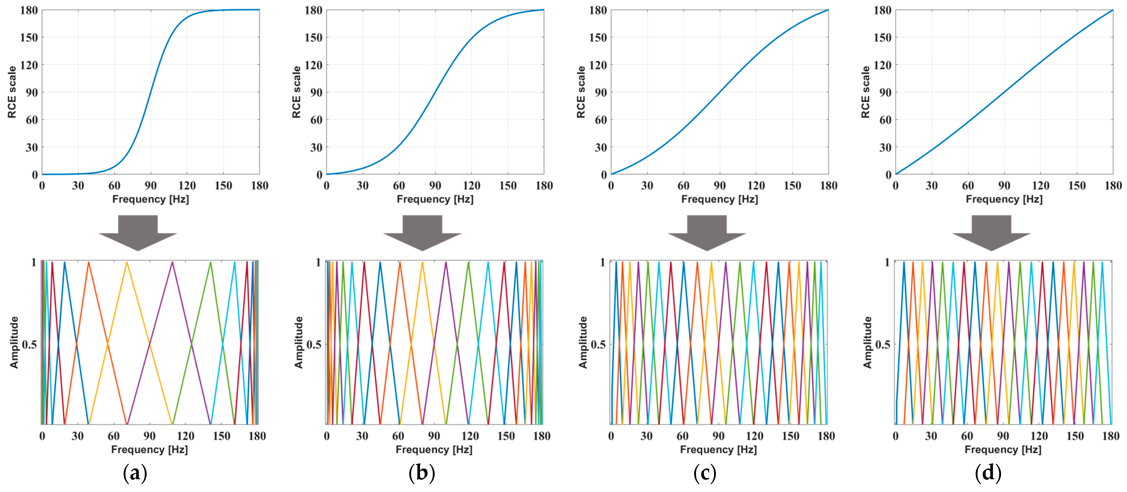
| Slope Factor | 0.1 | 0.2 | 0.3 | 0.4 | 0.5 | 0.6 | 0.7 | 0.8 | 0.9 | 1.0 | Mean | Std. | |
|---|---|---|---|---|---|---|---|---|---|---|---|---|---|
| Training | Accuracy | 84.38% | 82.81% | 84.38% | 93.75% | 99.38% | 95.31% | 90.63% | 82.81% | 71.11% | 67.36% | 85.19% | 9.671 |
| Loss | 0.3774 | 0.4123 | 0.4022 | 0.1233 | 0.0455 | 0.1207 | 0.2237 | 0.4744 | 0.7582 | 0.7939 | 0.3731 | 0.244 | |
| Test | Accuracy | 75.06% | 68.31% | 83.19% | 91.13% | 99.01% | 90.03% | 85.17% | 81.21% | 68.54% | 64.75% | 80.64% | 10.70 |
| Loss | 0.4995 | 0.5736 | 0.3980 | 0.1865 | 0.0691 | 0.2132 | 0.2626 | 0.5081 | 0.7547 | 0.9112 | 0.0691 | 0.252 |
| Image Size | 3 | 3 | 3 | 3 | 3 | 3 | 3 | 3 | Mean | Std. | |
|---|---|---|---|---|---|---|---|---|---|---|---|
| Training | Accuracy | 81.81% | 90.63% | 92.19% | 99.38% | 99.22% | 95.70% | 98.44% | 77.34% | 91.96% | 7.606 |
| Loss | 0.3995 | 0.2237 | 0.1980 | 0.0455 | 0.0465 | 0.1202 | 0.0995 | 0.5364 | 0.2087 | 0.165 | |
| Test | Accuracy | 75.06% | 83.58% | 93.64% | 99.01% | 99.14% | 95.31% | 97.59% | 75.06% | 89.80% | 9.688 |
| Loss | 0.5601 | 0.2626 | 0.1946 | 0.0691 | 0.0709 | 0.1350 | 0.0833 | 0.5616 | 0.2422 | 0.194 |
| Count | 1 | 2 | 3 | 4 | 5 | 6 | 7 | 8 | 9 | 10 | Mean | Std. | |
|---|---|---|---|---|---|---|---|---|---|---|---|---|---|
| Training | Accuracy | 100% | 98.44% | 99.22% | 100% | 99.22% | 99.22% | 100% | 99.22% | 99.22% | 99.22% | 99.38% | 0.469 |
| Loss | 0.0102 | 0.2268 | 0.0321 | 0.0124 | 0.0491 | 0.0318 | 0.0161 | 0.0161 | 0.0258 | 0.0349 | 0.0455 | 0.061 | |
| Test | Accuracy | 99.74% | 95.96% | 99.40% | 99.91% | 98.19% | 98.62% | 99.74% | 99.94% | 99.40% | 99.05% | 99.01% | 1.158 |
| Loss | 0.0182 | 0.1250 | 0.0579 | 0.0545 | 0.0577 | 0.0465 | 0.0863 | 0.0863 | 0.0684 | 0.0906 | 0.0691 | 0.028 |
| Actual | |||
|---|---|---|---|
| Fault | Normal | ||
| Predicted | Fault | 873 | 0 |
| Normal | 3 | 287 | |
| Actual | |||
|---|---|---|---|
| Fault | Normal | ||
| Predicted | Fault | 660 | 286 |
| Normal | 44 | 264 | |
| Actual | |||
|---|---|---|---|
| Fault | Normal | ||
| Predicted | Fault | 946 | 0 |
| Normal | 308 | 0 | |
| Actual | |||
|---|---|---|---|
| Fault | Normal | ||
| Predicted | Fault | 946 | 0 |
| Normal | 308 | 0 | |
| Image | RCE Spectrogram (Proposed) | Spectrogram | Mel Spectrogram | MFCC | |
|---|---|---|---|---|---|
| Metric | |||||
| Accuracy | 0.9974 | 0.7368 | 0.7544 | 0.7544 | |
| Recall | 0.9966 | 0.9375 | 0.7544 | 0.7544 | |
| Precision | 1.0000 | 0.6977 | 1.0000 | 1.0000 | |
| F1 score | 0.9983 | 0.8000 | 0.8600 | 0.8600 | |
Disclaimer/Publisher’s Note: The statements, opinions and data contained in all publications are solely those of the individual author(s) and contributor(s) and not of MDPI and/or the editor(s). MDPI and/or the editor(s) disclaim responsibility for any injury to people or property resulting from any ideas, methods, instructions or products referred to in the content. |
© 2024 by the authors. Licensee MDPI, Basel, Switzerland. This article is an open access article distributed under the terms and conditions of the Creative Commons Attribution (CC BY) license (https://creativecommons.org/licenses/by/4.0/).
Share and Cite
Seong, G.; Kim, D. An Intelligent Ball Bearing Fault Diagnosis System Using Enhanced Rotational Characteristics on Spectrogram. Sensors 2024, 24, 776. https://doi.org/10.3390/s24030776
Seong G, Kim D. An Intelligent Ball Bearing Fault Diagnosis System Using Enhanced Rotational Characteristics on Spectrogram. Sensors. 2024; 24(3):776. https://doi.org/10.3390/s24030776
Chicago/Turabian StyleSeong, Gyujin, and Dongwan Kim. 2024. "An Intelligent Ball Bearing Fault Diagnosis System Using Enhanced Rotational Characteristics on Spectrogram" Sensors 24, no. 3: 776. https://doi.org/10.3390/s24030776
APA StyleSeong, G., & Kim, D. (2024). An Intelligent Ball Bearing Fault Diagnosis System Using Enhanced Rotational Characteristics on Spectrogram. Sensors, 24(3), 776. https://doi.org/10.3390/s24030776