
Method of 3D Coating Accumulation Modeling Based on Inclined Spraying


Abstract
:1. Introduction
- The data are obtained by fixed-distance spraying. This method requires a large number of experiments, low data-acquisition efficiency, and insufficient data information.
- The β distribution model is relatively simple, and the ability to capture data features is weak. The coating thickness distribution model established by this method has low accuracy and weak adaptability.

| Reference | Modeling Method | Modeling Efficiency | Model Information Quantity | Model Accuracy | |
|---|---|---|---|---|---|
| Maximum Error | Average Relative Error | ||||
| Xue-mei, L. et al. [7] | β distribution model | The data density is insufficient, and the process of obtaining experimental data by fixed-distance spraying is complex. | The model is not intuitive enough to express the data, and the representation ability is weak. | 43.7 μm | -- |
| Guolei, W. et al. [8] | β distribution model | The spatial relationship of the model is considered, but the β distribution model is simple and the ability to capture data features is weak. | -- | 4.3% | |
| Yi, W. et al. [11] | Elliptical double β distribution model | The data density is limited, and the collection efficiency is low for the data collection of flat plate fixed-distance spraying. | Compared with the β model, the elliptical double β model increases the complexity and expression ability of modeling, but the model established by fixed-distance spraying lacks the ability to adapt to any surface spraying. | 2.8 μm | -- |
| Shulin, Q. et al. [12] | Elliptical double β distribution model | 3.7 μm | -- | ||
| Yong, Z. et al. [13] | Parabolic distribution model | The fixed-distance experiment obtains data, and the modeling efficiency is low. | Considering the posture of the spray gun, and taking the spraying distance and spraying angle into account in the algorithm, it has a certain adaptability. | 3.6 μm | -- |
| Chen, C. et al. [14] | Gaussian distribution model | The data acquisition method of fixed-distance spraying is complex, and the data coverage is insufficient. | The model lacks spatial information expression. | -- | 25.2% |
| Wu, H. et al. [15] | Gaussian distribution model of 3D | Compared with the 2D Gaussian model, the 3D model can describe the coating accumulation more accurately and improve the accuracy of the model. | -- | 7.6% | |
| Hua, R.-X. et al. [16] | Rectangular distribution model of 3D | The process of data acquisition is complex, and the amount of information is insufficient. | The 3D rectangular coating thickness distribution model is adopted, and the accuracy is high. | 10.0 μm | -- |
2. Establishing Model
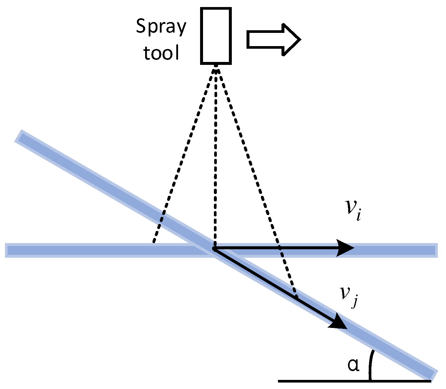
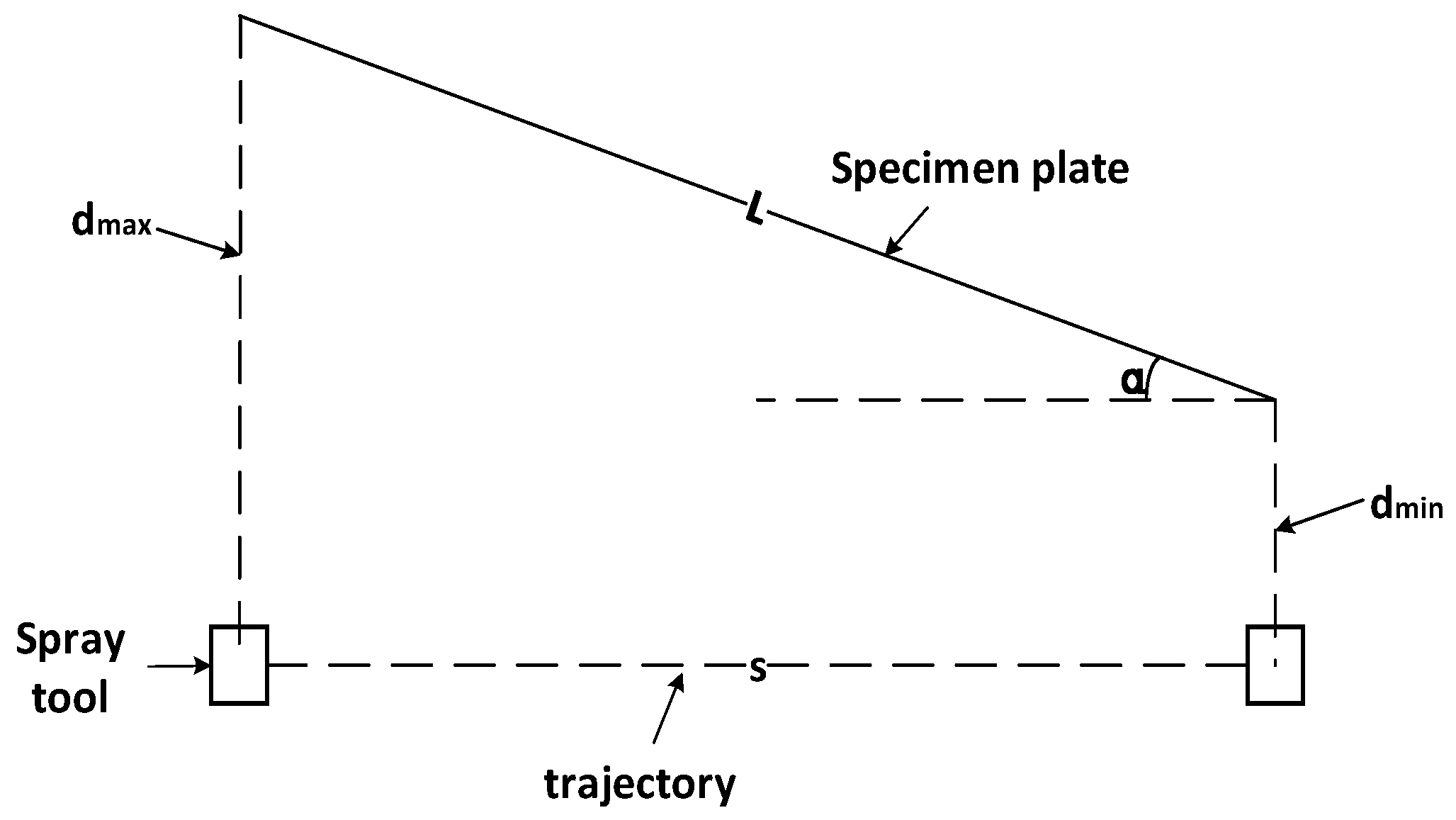
2.1. Accumulation Model of Oblique Spray Coating
2.2. Generation of Model Training Data
2.3. 3D Coating Accumulation Model
3. Verification Method
3.1. Verify the Oblique Spraying Coating Accumulation Model
3.2. 3D Coating Accumulation Model Training and Verification
4. Results
4.1. Verification Results of Oblique Spray Coating Accumulation Model
4.2. Validation Results of 3D Coating Accumulation Model
5. Discussion
- (1)
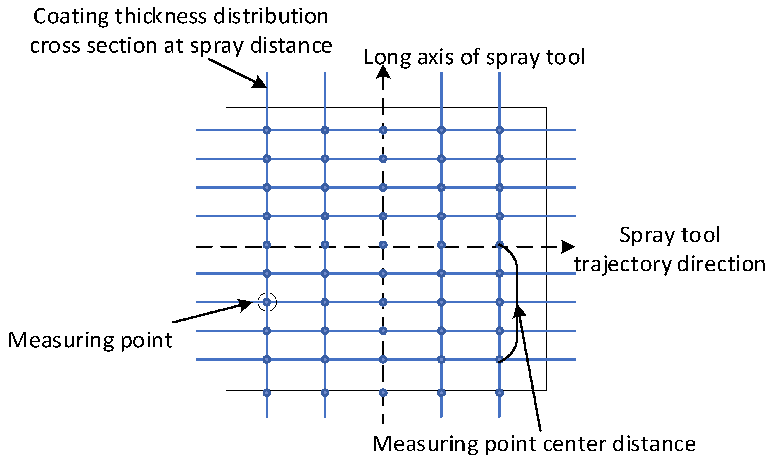
- For the performance of the oblique spraying layer accumulation model, it can be seen from the coating surface quality of the oblique spraying experimental template in Figure 9 and the fixed-distance spraying experimental template in Figure 10, there is no sagging phenomenon on the surface of the sample with the minimum spraying distance of 170 mm, and the coating coverage is completed on the surface of the sample with the maximum spraying distance of 290 mm, which conforms to the distribution law of the middle thick edge thin. It can be seen from Figure 12 that the calculated value of the model is consistent with the thickness change trend of the actual value. It can be seen from Table A1, Table A2 and Table A3 in Appendix A that the absolute errors of the three spray distances are −1.3~2 μm, −1.9~2.2 μm, and −1.6~1.4 μm, respectively, when the center distance of the measuring point is in the range of −80~80 mm. The absolute errors and the relative errors of the three spray distances are large when the center distance of the measuring point is in the range of −150~−90 mm and 90~150 mm. This is because the coating in the edge area of the spray is thin, and a small thickness difference will also produce a large relative error. From Table 5, the relative error is small when the center distance of the measurement point is in the range of 80~80 mm, and the average relative error of the same spray distance is relatively close on the three oblique spray test samples. The range of average relative error is (4.22 ± 0.21)% when the spray distance is 170 mm, the range of average relative error is (3.78 ± 0.08)% when the spray distance is 250 mm, and the range of average relative error is (4.29 ± 0.07)% when the spray distance is 290 mm.
- (2)
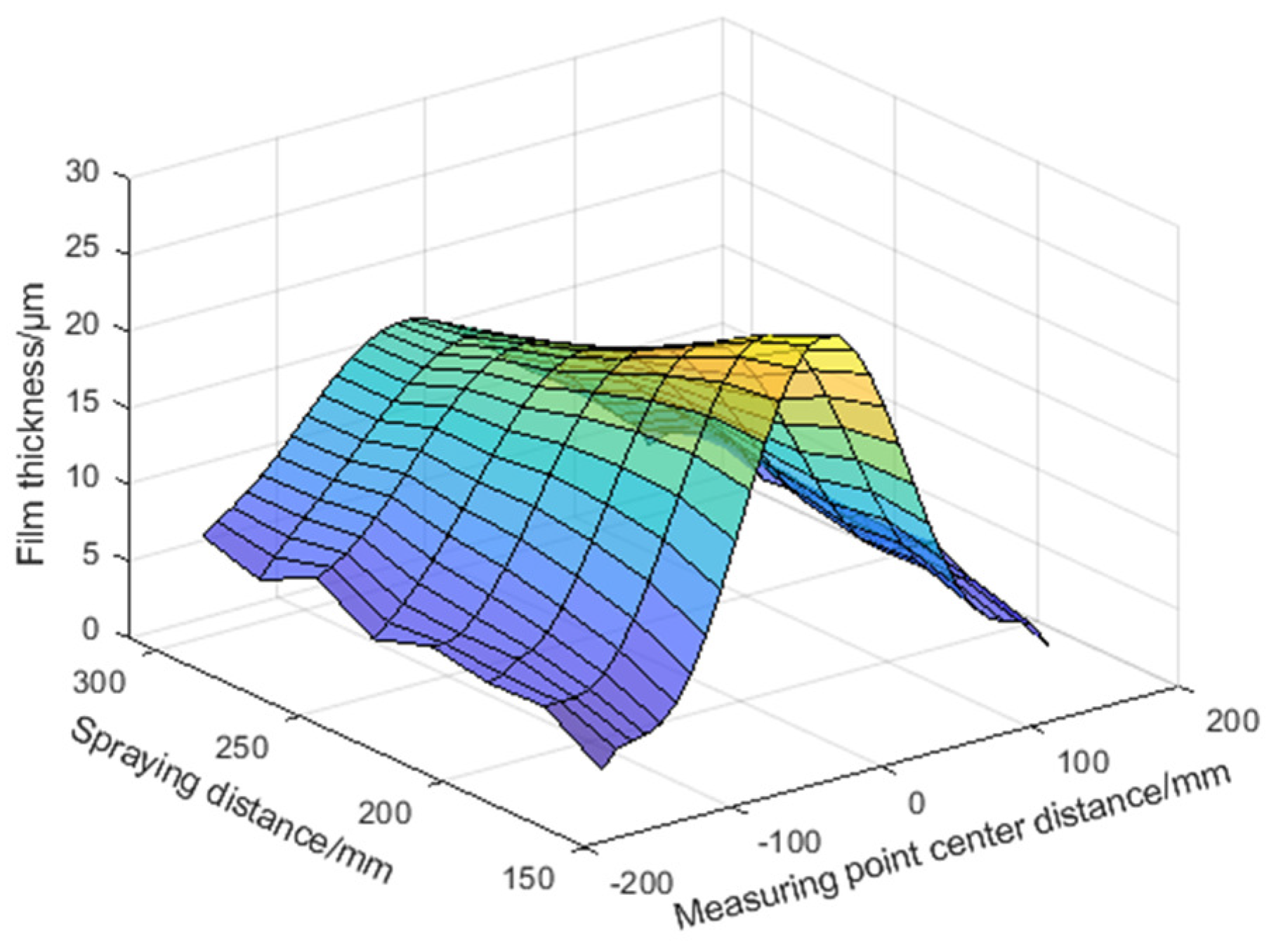
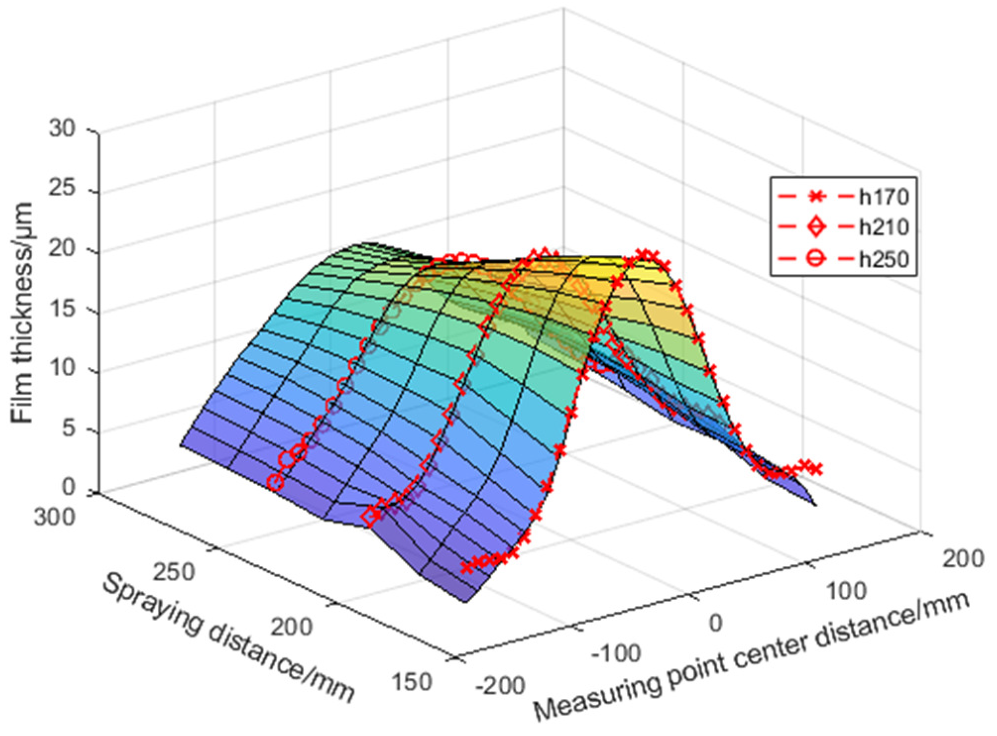
- The performance of the 3D coating accumulation model can be seen in Table A4, Table A5 and Table A6 in Appendix A. Within the center distance of the measurement point of −150~150 mm, the absolute errors of the coating thickness predicted by the model for the spraying distance of 170 mm, 210 mm, and 250 mm are −0.9~2.4 μm, −0.5~1.8 μm, and 0~1.2 μm, respectively, and the average relative errors are 9.7%, 3.7%, and 4.5%, respectively. The center distance of the measuring point is close to the edge of the spray, such as the center distance of the measuring point is −150 mm and 150 mm, the error and relative error become larger, because in the edge part, the coating quality decreases and the thickness is not uniform, which affects the prediction accuracy of the model. According to Figure 13, the expression of the thickness change trend of the output value of the model is consistent with the actual value in space.
6. Conclusions
- (1)
- A method for establishing the accumulation model of oblique spraying coating was proposed. This method can realize the rapid acquisition of coating thickness data at any spray distance within the range of spray distance set by the experimental sample and has efficient data acquisition ability and the ability to extract high-density valuable information.
- (2)
- In the range of spraying distance 170~290 mm, the average relative error of the model is less than 4.1%, which can realize the efficient generation of training data of the 3D coating cumulative model. The model has good applicability and accuracy in the range of 80~80 mm from the center distance of the measurement point.
- (3)
- In this paper, a 3D coating accumulation model with coating as a function is established with spraying distance and spraying position as variables. The accuracy of the model is 1.2% and 21.5% higher than that of the two similar models. Using this model, the coating thickness can be accurately calculated according to the spraying distance and spraying position, so as to improve the coating simulation accuracy in the spraying simulation software.
Author Contributions
Funding
Institutional Review Board Statement
Informed Consent Statement
Data Availability Statement
Conflicts of Interest
Appendix A
| Measuring Point Center Distance/mm | /μm | /μm | /μm | /μm | Absolute Error/μm | Relative Error/% | ||||
|---|---|---|---|---|---|---|---|---|---|---|
| −150 | 4.3 | 2.6 | 2.5 | 3.1 | −1.7 | −1.8 | −1.2 | 38.89 | 41.66 | 27.77 |
| −140 | 4.6 | 2.2 | 3.2 | 3.0 | −2.4 | −1.4 | −1.6 | 52.47 | 30.00 | 35.19 |
| −130 | 4.4 | 3.1 | 4.3 | 3.7 | −1.4 | −0.1 | −0.7 | 30.70 | 2.80 | 16.30 |
| −120 | 4.3 | 4.2 | 8.3 | 3.0 | −0.1 | 4.0 | −1.3 | 1.51 | 93.29 | 30.97 |
| −110 | 4.6 | 3.8 | 3.9 | 4.6 | −0.8 | −0.7 | 0.0 | 17.31 | 15.60 | 0.25 |
| −100 | 5.6 | 4.8 | 7.3 | 6.3 | −0.8 | 1.6 | 0.7 | 13.82 | 29.27 | 12.32 |
| −90 | 7.2 | 8.4 | 6.9 | 7.7 | 1.2 | −0.3 | 0.5 | 16.24 | 4.60 | 6.92 |
| −80 | 9.4 | 8.6 | 9.6 | 9.6 | −0.8 | 0.2 | 0.2 | 8.42 | 2.08 | 2.08 |
| −70 | 12.1 | 11.6 | 12.2 | 11.5 | −0.5 | 0.2 | −0.6 | 3.91 | 1.33 | 4.57 |
| −60 | 15.0 | 14.2 | 14.6 | 14.2 | −0.8 | −0.4 | −0.8 | 5.61 | 2.44 | 5.61 |
| −50 | 17.9 | 17.6 | 17.6 | 16.8 | −0.3 | −0.3 | −1.2 | 1.88 | 1.88 | 6.52 |
| −40 | 20.7 | 19.6 | 18.8 | 19.7 | −1.1 | −1.9 | −1.0 | 5.43 | 9.26 | 4.66 |
| −30 | 23.1 | 22.1 | 21.5 | 22.5 | −1.0 | −1.6 | −0.6 | 4.23 | 6.81 | 2.69 |
| −20 | 24.9 | 24.5 | 25.7 | 23.4 | −0.5 | 0.7 | −1.5 | 1.93 | 3.00 | 6.06 |
| −10 | 26.1 | 26.5 | 27.2 | 24.5 | 0.4 | 1.1 | −1.6 | 1.44 | 4.33 | 6.15 |
| 0 | 26.5 | 28.5 | 27.5 | 27.9 | 2.0 | 1.0 | 1.4 | 7.51 | 3.62 | 5.41 |
| 10 | 26.1 | 28.1 | 28.3 | 25.6 | 1.9 | 2.2 | −0.6 | 7.39 | 8.30 | 2.17 |
| 20 | 25.0 | 25.0 | 24.7 | 23.4 | 0.0 | −0.3 | −1.6 | 0.13 | 1.08 | 6.31 |
| 30 | 23.2 | 22.4 | 21.8 | 23.1 | −0.8 | −1.4 | −0.1 | 3.32 | 6.22 | 0.58 |
| 40 | 20.9 | 19.7 | 19.6 | 20.3 | −1.2 | −1.2 | −0.5 | 5.60 | 5.97 | 2.56 |
| 50 | 18.2 | 16.9 | 17.5 | 19.3 | −1.3 | −0.7 | 1.1 | 7.04 | 3.77 | 6.05 |
| 60 | 15.3 | 14.2 | 14.7 | 15.5 | −1.1 | −0.6 | 0.2 | 7.24 | 3.61 | 1.06 |
| 70 | 12.5 | 12.9 | 12.1 | 13.0 | 0.4 | −0.4 | 0.5 | 3.54 | 2.81 | 3.86 |
| 80 | 9.9 | 10.0 | 10.5 | 10.1 | 0.1 | 0.5 | 0.2 | 0.66 | 5.45 | 1.86 |
| 90 | 7.8 | 8.2 | 9.9 | 9.2 | 0.4 | 2.1 | 1.3 | 4.52 | 26.34 | 17.20 |
| 100 | 6.3 | 6.9 | 5.0 | 8.3 | 0.6 | −1.3 | 2.0 | 9.81 | 20.48 | 32.54 |
| 110 | 5.4 | 4.9 | 7.0 | 4.3 | −0.5 | 1.6 | −1.1 | 8.71 | 30.31 | 20.49 |
| 120 | 5.1 | 3.9 | 5.9 | 3.0 | −1.1 | 0.9 | −2.1 | 22.58 | 17.31 | 41.35 |
| 130 | 5.1 | 4.7 | 3.3 | 1.7 | −0.4 | −1.8 | −3.5 | 8.16 | 35.17 | 67.59 |
| 140 | 5.2 | 3.9 | 3.0 | 5.0 | −1.3 | −2.2 | −0.2 | 25.39 | 42.90 | 4.07 |
| 150 | 4.7 | 2.9 | 2.9 | 1.9 | −1.8 | −1.8 | −2.8 | 38.12 | 38.97 | 59.31 |
| Measuring Point Center Distance/mm | /μm | /μm | /μm | /μm | Absolute Error/μm | Relative Error/% | ||||
|---|---|---|---|---|---|---|---|---|---|---|
| −150 | 4.2 | 4.1 | 5.0 | 2.4 | 0.0 | 0.8 | −1.8 | 0.66 | 20.35 | 42.69 |
| −140 | 5.8 | 4.5 | 4.4 | 5.0 | −1.3 | −1.4 | −0.8 | 22.41 | 24.45 | 14.24 |
| −130 | 6.1 | 4.6 | 5.1 | 3.7 | −1.5 | −1.0 | −2.4 | 24.22 | 16.45 | 39.77 |
| −120 | 6.9 | 5.9 | 6.1 | 5.6 | −1.0 | −0.8 | −1.3 | 14.13 | 11.82 | 18.74 |
| −110 | 8.0 | 9.1 | 10.5 | 6.1 | 1.2 | 2.5 | −1.9 | 14.55 | 31.48 | 23.80 |
| −100 | 9.2 | 8.4 | 9.0 | 8.6 | −0.8 | −0.2 | −0.7 | 9.13 | 2.27 | 7.42 |
| −90 | 10.6 | 11.5 | 10.7 | 10.5 | 0.8 | 0.1 | −0.2 | 7.98 | 0.54 | 1.70 |
| −80 | 12.1 | 12.8 | 12.6 | 12.5 | 0.7 | 0.5 | 0.4 | 5.75 | 4.44 | 3.45 |
| −70 | 13.5 | 14.4 | 12.8 | 13.1 | 1.0 | −0.6 | −0.4 | 7.26 | 4.52 | 2.76 |
| −60 | 14.7 | 14.8 | 14.9 | 14.2 | 0.1 | 0.1 | −0.6 | 0.60 | 0.87 | 3.97 |
| −50 | 15.9 | 15.2 | 15.7 | 14.9 | −0.7 | −0.2 | −1.0 | 4.15 | 1.16 | 6.40 |
| −40 | 16.8 | 16.4 | 17.0 | 16.4 | −0.4 | 0.2 | −0.4 | 2.60 | 0.93 | 2.60 |
| −30 | 17.6 | 17.6 | 17.1 | 17.6 | −0.1 | −0.5 | 0.0 | 0.31 | 2.79 | 0.09 |
| −20 | 18.2 | 18.8 | 19.0 | 19.0 | 0.6 | 0.9 | 0.9 | 3.46 | 4.77 | 4.77 |
| −10 | 18.5 | 18.7 | 18.4 | 19.0 | 0.2 | 0.0 | 0.6 | 1.05 | 0.24 | 2.98 |
| 0 | 18.6 | 19.5 | 20.2 | 18.4 | 0.9 | 1.7 | −0.1 | 5.10 | 8.95 | 0.66 |
| 10 | 18.4 | 19.4 | 19.0 | 17.6 | 1.0 | 0.6 | −0.8 | 5.35 | 3.41 | 4.34 |
| 20 | 18.0 | 18.3 | 18.8 | 17.6 | 0.3 | 0.8 | −0.4 | 1.66 | 4.30 | 2.30 |
| 30 | 17.4 | 17.4 | 18.6 | 15.9 | 0.0 | 1.1 | −1.5 | 0.17 | 6.54 | 8.48 |
| 40 | 16.6 | 15.8 | 17.6 | 15.7 | −0.8 | 1.0 | −0.9 | 5.02 | 5.96 | 5.50 |
| 50 | 15.6 | 15.2 | 14.7 | 15.7 | −0.4 | −0.9 | 0.1 | 2.63 | 5.67 | 0.41 |
| 60 | 14.5 | 13.4 | 14.0 | 13.8 | −1.1 | −0.5 | −0.7 | 7.37 | 3.27 | 4.91 |
| 70 | 13.3 | 12.3 | 12.7 | 12.2 | −1.0 | −0.5 | −1.0 | 7.41 | 4.12 | 7.71 |
| 80 | 12.0 | 11.3 | 11.8 | 11.97 | −0.7 | −0.3 | −0.2 | 5.61 | 2.63 | 1.64 |
| 90 | 10.7 | 10.5 | 11.1 | 9.0 | −0.2 | 0.4 | −1.6 | 1.75 | 3.83 | 15.15 |
| 100 | 9.4 | 9.5 | 11.1 | 8.7 | 0.1 | 1.7 | −0.7 | 1.41 | 17.89 | 7.46 |
| 110 | 8.2 | 8.9 | 10.5 | 9.6 | 0.6 | 2.2 | 1.4 | 7.88 | 27.14 | 17.03 |
| 120 | 7.3 | 8.1 | 9.0 | 4.8 | 0.8 | 1.8 | −2.5 | 11.53 | 24.04 | 34.72 |
| 130 | 6.6 | 6.9 | 5.9 | 7.8 | 0.3 | −0.7 | 1.2 | 4.37 | 10.54 | 18.09 |
| 140 | 6.4 | 5.8 | 5.2 | 2.9 | −0.6 | −1.2 | −3.6 | 9.95 | 18.59 | 55.59 |
| 150 | 6.8 | 5.0 | 6.5 | 4.8 | −1.7 | −0.2 | −2.0 | 25.54 | 3.26 | 29.65 |
| Measuring Point Center Distance/mm | /μm | /μm | /μm | /μm | Absolute Error/μm | Relative Error/% | ||||
|---|---|---|---|---|---|---|---|---|---|---|
| −150 | 6.1 | 5.1 | 5.1 | 5.9 | −1.0 | −1.0 | −0.2 | 17.01 | 16.36 | 2.75 |
| −140 | 6.6 | 6.5 | 10.3 | 3.4 | −0.1 | 3.8 | −3.1 | 1.34 | 57.02 | 47.66 |
| −130 | 7.3 | 5.6 | 7.0 | 3.7 | −1.7 | −0.3 | −3.6 | 23.20 | 3.59 | 49.35 |
| −120 | 8.1 | 7.4 | 6.3 | 8.3 | −0.7 | −1.8 | 0.2 | 8.69 | 22.37 | 2.54 |
| −110 | 9.1 | 9.6 | 12.2 | 5.6 | 0.5 | 3.2 | −3.5 | 5.48 | 35.24 | 38.29 |
| −100 | 10.0 | 9.7 | 10.8 | 7.4 | −0.3 | 0.8 | −2.7 | 3.33 | 7.72 | 26.61 |
| −90 | 11.0 | 11.9 | 12.1 | 10.1 | 0.8 | 1.1 | −0.9 | 7.65 | 9.81 | 8.50 |
| −80 | 12.0 | 12.5 | 12.8 | 11.3 | 0.5 | 0.8 | −0.7 | 3.85 | 6.82 | 6.04 |
| −70 | 12.9 | 13.4 | 13.4 | 12.5 | 0.5 | 0.5 | −0.5 | 3.78 | 3.78 | 3.57 |
| −60 | 13.8 | 14.2 | 14.7 | 13.0 | 0.4 | 0.9 | −0.8 | 2.57 | 6.88 | 6.05 |
| −50 | 14.2 | 14.7 | 15.0 | 13.7 | 0.5 | 0.8 | −0.5 | 3.70 | 5.37 | 3.83 |
| −40 | 15.2 | 14.6 | 15.7 | 14.6 | −0.6 | 0.5 | −0.6 | 3.96 | 3.35 | 3.70 |
| −30 | 15.7 | 16.1 | 16.4 | 14.9 | 0.4 | 0.7 | −0.8 | 2.49 | 4.51 | 5.33 |
| −20 | 16.1 | 16.4 | 16.6 | 15.3 | 0.3 | 0.6 | −0.7 | 1.80 | 3.52 | 4.61 |
| −10 | 16.3 | 17.0 | 17.2 | 16.3 | 0.7 | 0.9 | 0.0 | 4.20 | 5.66 | 0.17 |
| 0 | 16.4 | 17.5 | 17.5 | 16.3 | 1.1 | 1.1 | −0.1 | 6.52 | 6.52 | 0.73 |
| 10 | 16.4 | 17.2 | 17.6 | 15.5 | 0.9 | 1.2 | −0.9 | 5.43 | 7.61 | 5.48 |
| 20 | 16.2 | 16.5 | 16.3 | 15.2 | 0.4 | 0.1 | −0.9 | 2.33 | 0.86 | 5.77 |
| 30 | 15.8 | 16.1 | 15.5 | 15.0 | 0.3 | −0.3 | −0.8 | 2.06 | 2.20 | 5.21 |
| 40 | 15.3 | 14.3 | 15.0 | 14.3 | −1.1 | −0.3 | −1.1 | 6.88 | 2.23 | 6.88 |
| 50 | 14.7 | 14.7 | 14.9 | 14.0 | 0.0 | 0.2 | −0.7 | 0.22 | 1.03 | 4.63 |
| 60 | 14.0 | 12.8 | 13.9 | 13.3 | −1.2 | −0.1 | −0.7 | 8.45 | 0.51 | 4.76 |
| 70 | 13.2 | 12.2 | 12.0 | 12.8 | −0.9 | −1.1 | −0.3 | 6.88 | 8.69 | 2.36 |
| 80 | 12.2 | 11.4 | 11.8 | 11.7 | −0.8 | −0.5 | −0.6 | 6.70 | 3.79 | 4.76 |
| 90 | 11.3 | 8.8 | 8.8 | 8.6 | −2.4 | −2.5 | −2.7 | 21.47 | 21.82 | 23.93 |
| 100 | 10.2 | 7.7 | 7.7 | 7.7 | −2.5 | −2.5 | −2.5 | 24.88 | 24.49 | 24.49 |
| 110 | 9.2 | 6.7 | 5.9 | 5.7 | −2.5 | −3.3 | −3.5 | 26.84 | 35.45 | 38.03 |
| 120 | 8.2 | 8.8 | 11.1 | 7.4 | 0.5 | 2.8 | −0.8 | 6.67 | 34.67 | 10.22 |
| 130 | 7.3 | 6.9 | 7.6 | 4.3 | −0.4 | 0.3 | −3.0 | 5.84 | 4.50 | 41.22 |
| 140 | 6.5 | 8.8 | 10.5 | 5.9 | 2.3 | 4.0 | −0.5 | 35.99 | 61.72 | 8.12 |
| 150 | 5.8 | 7.0 | 9.6 | 4.6 | 1.2 | 3.8 | −1.2 | 20.33 | 65.19 | 20.46 |
| Measuring Point Center Distance/mm | Coating Thickness/μm | Absolute Error/μm | Relative Error/% | |
|---|---|---|---|---|
| True Value | Predict Value | |||
| −150 | 4.3 | 2 | 2.3 | 53.3 |
| −140 | 4.6 | 3.1 | 1.5 | 32.4 |
| −130 | 4.4 | 3.4 | 1.0 | 22.8 |
| −120 | 4.3 | 3.6 | 0.7 | 16.4 |
| −110 | 4.6 | 4 | 0.6 | 14.0 |
| −100 | 5.6 | 5.1 | 0.5 | 9.1 |
| −90 | 7.2 | 6.7 | 0.5 | 7.3 |
| −80 | 9.4 | 9 | 0.4 | 4.6 |
| −70 | 12.1 | 11.7 | 0.4 | 3.2 |
| −60 | 15.0 | 14.6 | 0.4 | 2.6 |
| −50 | 17.9 | 17.7 | 0.2 | 1.3 |
| −40 | 20.7 | 20.5 | 0.2 | 1.0 |
| −30 | 23.1 | 23.6 | −0.5 | 2.2 |
| −20 | 24.9 | 25.3 | −0.4 | 1.4 |
| −10 | 26.1 | 25.9 | 0.2 | 0.8 |
| 0 | 26.5 | 26.1 | 0.4 | 1.6 |
| 10 | 26.1 | 25.5 | 0.6 | 2.4 |
| 20 | 25.0 | 25.1 | −0.1 | 0.4 |
| 30 | 23.2 | 23.8 | −0.6 | 2.6 |
| 40 | 20.9 | 21.8 | −0.9 | 4.5 |
| 50 | 18.2 | 18.5 | −0.3 | 1.8 |
| 60 | 15.3 | 15.1 | 0.2 | 1.3 |
| 70 | 12.5 | 12.3 | 0.2 | 1.4 |
| 80 | 9.9 | 9.8 | 0.1 | 1.3 |
| 90 | 7.8 | 7.6 | 0.2 | 2.7 |
| 100 | 6.3 | 6.1 | 0.2 | 2.9 |
| 110 | 5.4 | 5.1 | 0.3 | 5.3 |
| 120 | 5.1 | 4.7 | 0.4 | 7.3 |
| 130 | 5.1 | 4.4 | 0.7 | 14.3 |
| 140 | 5.2 | 3.8 | 1.4 | 27.0 |
| 150 | 4.7 | 2.3 | 2.4 | 50.8 |
| Average | 9.7 | |||
| Measuring Point Center Distance/mm | Coating Thickness/μm | Absolute Error/μm | Relative Error | |
|---|---|---|---|---|
| True Value | Predict Value | |||
| −150 | 4.9 | 4.0 | 0.89 | 18.1 |
| −140 | 5.3 | 5.5 | 0.19 | 3.6 |
| −130 | 5.6 | 5.5 | 0.10 | 1.8 |
| −120 | 5.6 | 5.8 | 0.10 | 1.8 |
| −110 | 6.5 | 6.6 | 0.11 | 1.7 |
| −100 | 7.9 | 8.0 | 0.13 | 1.6 |
| −90 | 9.7 | 9.8 | 0.13 | 1.3 |
| −80 | 11.7 | 11.8 | 0.11 | 1.0 |
| −70 | 13.9 | 14.0 | 0.10 | 0.7 |
| −60 | 16.0 | 16.1 | 0.07 | 0.4 |
| −50 | 18.1 | 18.1 | 0.03 | 0.2 |
| −40 | 19.8 | 19.8 | 0.02 | 0.1 |
| −30 | 21.2 | 21.2 | 0.06 | 0.3 |
| −20 | 22.2 | 22.1 | 0.06 | 0.3 |
| −10 | 22.7 | 22.7 | 0.00 | 0.0 |
| 0 | 22.6 | 22.7 | 0.14 | 0.6 |
| 10 | 22.0 | 22.4 | 0.31 | 1.4 |
| 20 | 21.0 | 21.5 | 0.48 | 2.3 |
| 30 | 19.6 | 20.2 | 0.58 | 3.0 |
| 40 | 17.9 | 18.5 | 0.63 | 3.5 |
| 50 | 15.9 | 16.5 | 0.64 | 4.0 |
| 60 | 13.9 | 14.5 | 0.67 | 4.8 |
| 70 | 12.5 | 12.6 | 0.08 | 0.6 |
| 80 | 11.2 | 10.8 | 0.37 | 3.3 |
| 90 | 10.0 | 9.3 | 0.70 | 7.0 |
| 100 | 8.4 | 8.0 | 0.37 | 4.4 |
| 110 | 7.5 | 7.0 | 0.55 | 7.3 |
| 120 | 6.9 | 6.3 | 0.69 | 9.9 |
| 130 | 6.1 | 5.9 | 0.18 | 3.0 |
| 140 | 5.7 | 5.7 | 0.00 | 0.1 |
| 150 | 4.6 | 3.4 | 1.20 | 26.1 |
| Average | 3.7 | |||
| Measuring Point Center Distance/mm | Coating Thickness/μm | Absolute Error/μm | Relative Error | |
|---|---|---|---|---|
| True Value | Predict Value | |||
| −150 | 4.15 | 3.7 | 0.5 | 10.8 |
| −140 | 5.82 | 4.6 | 1.2 | 21.0 |
| −130 | 6.12 | 5.5 | 0.6 | 10.1 |
| −120 | 6.88 | 6.6 | 0.3 | 4.0 |
| −110 | 7.96 | 7.8 | 0.2 | 2.0 |
| −100 | 9.25 | 9.2 | 0.0 | 0.5 |
| −90 | 10.65 | 10.7 | −0.1 | 0.5 |
| −80 | 12.07 | 12.2 | −0.1 | 1.1 |
| −70 | 13.45 | 13.6 | −0.1 | 1.1 |
| −60 | 14.74 | 15 | −0.3 | 1.8 |
| −50 | 15.88 | 16.3 | −0.4 | 2.6 |
| −40 | 16.85 | 17.3 | −0.5 | 2.7 |
| −30 | 17.62 | 18.1 | −0.5 | 2.8 |
| −20 | 18.16 | 18.7 | −0.5 | 3.0 |
| −10 | 18.48 | 18.9 | −0.4 | 2.3 |
| 0 | 18.56 | 18.9 | −0.3 | 1.9 |
| 10 | 18.40 | 18.5 | −0.1 | 0.5 |
| 20 | 18.01 | 18 | 0.0 | 0.1 |
| 30 | 17.41 | 17.1 | 0.3 | 1.8 |
| 40 | 16.61 | 16.1 | 0.5 | 3.1 |
| 50 | 15.63 | 15 | 0.6 | 4.0 |
| 60 | 14.51 | 13.8 | 0.7 | 4.9 |
| 70 | 13.27 | 12.6 | 0.7 | 5.1 |
| 80 | 11.97 | 11.5 | 0.5 | 3.9 |
| 90 | 10.65 | 10.4 | 0.3 | 2.4 |
| 100 | 9.38 | 9.4 | 0.0 | 0.2 |
| 110 | 8.23 | 8.6 | −0.4 | 4.5 |
| 120 | 7.29 | 7.8 | −0.5 | 7.0 |
| 130 | 6.65 | 7 | −0.4 | 5.3 |
| 140 | 6.43 | 6.2 | 0.2 | 3.5 |
| 150 | 6.76 | 5 | 1.8 | 26.1 |
| Average | 4.5 | |||
References
- Antonio, J.K.; Ramabhadran, R.; Ling, T.L. A framework for optimal trajectory planning for automated spray coating. Int. J. Robot. Autom. 1997, 12, 124–133. [Google Scholar]
- Tokunaga, H.; Okano, T.; Matsuki, N.; Tanaka, F.; Kishinami, T. A Method to Solve Inverse Kinematics Problems Using Lie Algebra and Its Application to Robot Spray Painting Simulation. In Proceedings of the ASME 2004 International Design Engineering Technical Conferences and Computers and Information in Engineering Conference, Salt Lake City, UT, USA, 28 September–2 October 2004. [Google Scholar]
- Zeng, Y.; Zhang, Y.; He, J.; Zhou, H.; Zhang, C.; Zheng, L. Prediction model of coating growth rate for varied dip-angle spraying based on gaussian sum model. Math. Probl. Eng. 2016, 2016, 9369047. [Google Scholar] [CrossRef]
- Zhang, M. Brief Introduction of Film Thickness Control During Paint Spraying by Robot. Xiandai Tuliao Yu Tuzhuang 2006, 6, 31. [Google Scholar]
- Arkan, M.A.S.; Balkan, T. Process modeling, simulation, and paint thickness measurement for robotic spray painting. J. Robot. Syst. 2000, 17, 479–494. [Google Scholar] [CrossRef]
- Yonggui, Z.; Yumei, H.; Feng, G.; Wei, W. New model for air spray gun of robotic spray-painting. J. Mech. Eng. 2006, 42, 226–233. [Google Scholar]
- Suh, S.-H.; Woo, I.-K.; Noh, S.-K. Development of an automatic trajectory planning system (ATPS) for spray painting robots. In Proceedings of the 1991 IEEE International Conference on Robotics and Automation, Sacramento, CA, USA, 9–11 April 1991. [Google Scholar]
- Liu, X.-M.; Liu, T.; Yang, L.-S. Spray painting film thickness distribution on panel and optimization of width of paint film overlay. Surf. Technol. 2018, 47, 116–125. [Google Scholar]
- Wang, G.; Yi, Q.; Miao, D.; Chen, K.; Wang, L. Multivariable coating thickness distribution model for robotic spray painting. J. Tsinghua Univ. (Sci. Technol.) 2017, 57, 324–330. [Google Scholar]
- Zhou, Y.; Ma, S.; Li, A.; Yang, L. Path planning for spray painting robot of horns surfaces in ship manufacturing. IOP Conf. Ser. Mater. Sci. Eng. 2019, 521, 012015. [Google Scholar] [CrossRef]
- Nieto Bastida, S.; Lin, C.-Y. Autonomous Trajectory Planning for Spray Painting on Complex Surfaces Based on a Point Cloud Model. Sensors 2023, 23, 9634. [Google Scholar] [CrossRef] [PubMed]
- Yi, W.; Guolei, W.; Bo, L.; Jiyu, Y.; Dunmin, L. Analysis of Coating Uniformity in Boundary Zone of Surface Spraying with Large-size. Mech. Sci. Technol. Aerosp. Eng. 2022, 41, 1705–1712. [Google Scholar]
- Qi, S.; Zheng, Q.; Zhao, C.; Sun, Y.; Xia, H.; Jiang, D. Research on Trajectory Planning of Spraying Robot Based on Coating Thickness Model. Mach. Tool Hydraul. 2023, 51, 88–94. [Google Scholar]
- Shi, T.; Xu, J.; Cui, J.; Tao, L.; Xu, W.; Wang, Z.; Ji, J. Variable Velocity Coating Thickness Distribution Model for Super-Large Planar Robot Spraying. Coatings 2023, 13, 1434. [Google Scholar] [CrossRef]
- Hua, X.; Zhang, S.; Liu, X.; Chen, Z.; Wang, G.; Chen, K. Optimization of spraying trajectory based on elliptical double β spraying gun model. J. Tsinghua Univ. (Sci. Technol.) 2020, 60, 985–992. [Google Scholar]
- Zeng, Y.; Yu, Y.; Zhao, X.; Liu, Y.; Liu, J.; Liu, D. Trajectory Planning of Spray Gun With Variable Posture for Irregular Plane Based on Boundary Constraint. IEEE Access 2021, 9, 52902–52912. [Google Scholar] [CrossRef]
- Chen, C.; Xie, Y.; Verdy, C.; Liao, H.; Deng, S. Modelling of coating thickness distribution and its application in offline programming software. Surf. Coat. Technol. 2016, 318, 315–325. [Google Scholar] [CrossRef]
- Wu, H.; Xie, X.; Liu, M.; Chen, C.; Liao, H.; Zhang, Y.; Deng, S. A new approach to simulate coating thickness in cold spray. Surf. Coat. Technol. 2019, 382, 125151. [Google Scholar] [CrossRef]
- Hua, R.-X.; Zou, W.; Chen, G.-D.; Ma, H.-X.; Zhang, W. A model of spray tool and a parameter optimization method for spraying path planning. Int. J. Autom. Comput. 2021, 18, 1017–1031. [Google Scholar] [CrossRef]
- Gleeson, D.; Jakobsson, S.; Salman, R.; Sandgren, N.; Edelvik, F.; Carlson, J.S.; Lennartson, B. Robot spray painting trajectory optimization. In Proceedings of the 2020 IEEE 16th International Conference on Automation Science and Engineering (CASE), Hong Kong, China, 20–21 August 2020. [Google Scholar]
- Zhang, P.; Liu, J.; Chen, C.; Li, Y.Q. The algorithm study for using the back propagation neural network in CT image segmentation. In Proceedings of the International Conference on Innovative Optical Health Science, Shianghai, China, 10–12 October 2016. [Google Scholar]
- Yu, D.; Su, C.; Yang, D.; Bao, H. Prediction of spraying process parameters based on BP neural network. In Proceedings of the 2022 12th International Conference on CYBER Technology in Automation, Control, and Intelligent Systems (CYBER), Baishan, China, 27–31 July 2022. [Google Scholar]


| Transfer Function | R | Transfer Function | R | Transfer Function | R |
|---|---|---|---|---|---|
| 1-1-1 | 0.914 | 2-1-1 | 0.97 | 3-1-1 | 0.967 |
| 1-1-2 | 0.073 | 2-1-2 | 0.729 | 3-1-2 | 0.641 |
| 1-1-3 | 0.993 | 2-1-3 | 0.859 | 3-1-3 | 0.891 |
| 1-2-1 | 0.955 | 2-2-1 | 0.912 | 3-2-1 | 0.956 |
| Training Function | R | Training Function | R |
|---|---|---|---|
| Trainlm | 0.993 | Traincgf | 0.86 |
| Trainbr | 0.987 | Traincgp | 0.987 |
| Trainbfg | 0.261 | Trainoss | 0.973 |
| Trainrp | 0.98 | Traingdx | 0.871 |
| Trainscg | 0.986 | Traingdm | 0.982 |
| Traincgb | 0.929 | traingd | 0.983 |
| Measuring Point Center Distance/mm | h190/μm | h230/μm | h270/μm | h310/μm |
|---|---|---|---|---|
| −80 | 10.8 | 12.2 | 12.5 | 11.3 |
| −70 | 13.3 | 14.1 | 13.7 | 12.4 |
| −60 | 15.8 | 15.8 | 14.8 | 13.4 |
| −50 | 18.3 | 17.3 | 15.8 | 14.3 |
| −40 | 20.6 | 18.7 | 16.6 | 15.0 |
| −30 | 22.5 | 19.7 | 17.2 | 15.5 |
| −20 | 23.9 | 20.3 | 17.5 | 15.8 |
| −10 | 24.7 | 20.6 | 17.6 | 15.8 |
| 0 | 24.8 | 20.6 | 17.5 | 15.5 |
| 10 | 24.4 | 20.1 | 17.2 | 15.1 |
| 20 | 23.3 | 19.3 | 16.7 | 14.4 |
| 30 | 21.7 | 18.2 | 16.0 | 13.7 |
| 40 | 19.7 | 16.9 | 15.1 | 12.8 |
| 50 | 17.4 | 15.4 | 14.2 | 11.9 |
| 60 | 15.1 | 13.8 | 13.3 | 11.1 |
| 70 | 12.7 | 12.1 | 12.4 | 10.3 |
| 80 | 10.6 | 10.6 | 11.5 | 9.7 |
| Spraying Distance | Gi−1 | Gi−2 | Gi−3 | Average |
|---|---|---|---|---|
| h170 | 4.43% | 4.23% | 4.01% | 4.22% |
| h250 | 3.85% | 3.80% | 3.70% | 3.78% |
| h290 | 4.22% | 4.31% | 4.35% | 4.29% |
| Average | -- | -- | -- | 4.09% |
| Author and Year of Publication | Average Absolute Error | Average Relative Error |
|---|---|---|
| This work | 0.31 μm | 3.7% |
| Reference [6]: Guo lei, W. 2017 | 0.92 μm | 4.9% |
| Reference [13]: Chen, C. 2016 | -- | 25.2% |
Disclaimer/Publisher’s Note: The statements, opinions and data contained in all publications are solely those of the individual author(s) and contributor(s) and not of MDPI and/or the editor(s). MDPI and/or the editor(s) disclaim responsibility for any injury to people or property resulting from any ideas, methods, instructions or products referred to in the content. |
© 2024 by the authors. Licensee MDPI, Basel, Switzerland. This article is an open access article distributed under the terms and conditions of the Creative Commons Attribution (CC BY) license (https://creativecommons.org/licenses/by/4.0/).
Share and Cite
Yu, D.; Su, C.; Wang, E.; Bao, H.; Qu, F. Method of 3D Coating Accumulation Modeling Based on Inclined Spraying. Sensors 2024, 24, 1212. https://doi.org/10.3390/s24041212
Yu D, Su C, Wang E, Bao H, Qu F. Method of 3D Coating Accumulation Modeling Based on Inclined Spraying. Sensors. 2024; 24(4):1212. https://doi.org/10.3390/s24041212
Chicago/Turabian StyleYu, Danyang, Chengzhi Su, Enguo Wang, Haifeng Bao, and Fuheng Qu. 2024. "Method of 3D Coating Accumulation Modeling Based on Inclined Spraying" Sensors 24, no. 4: 1212. https://doi.org/10.3390/s24041212