
Feature Extraction of Lubricating Oil Debris Signal Based on Segmentation Entropy with an Adaptive Threshold


Abstract
1. Introduction
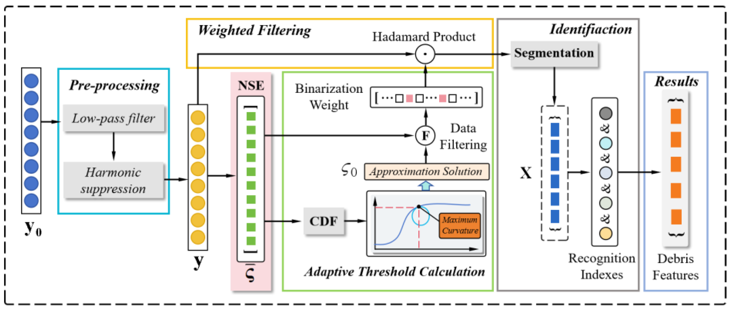
2. Debris Feature Extraction Algorithm
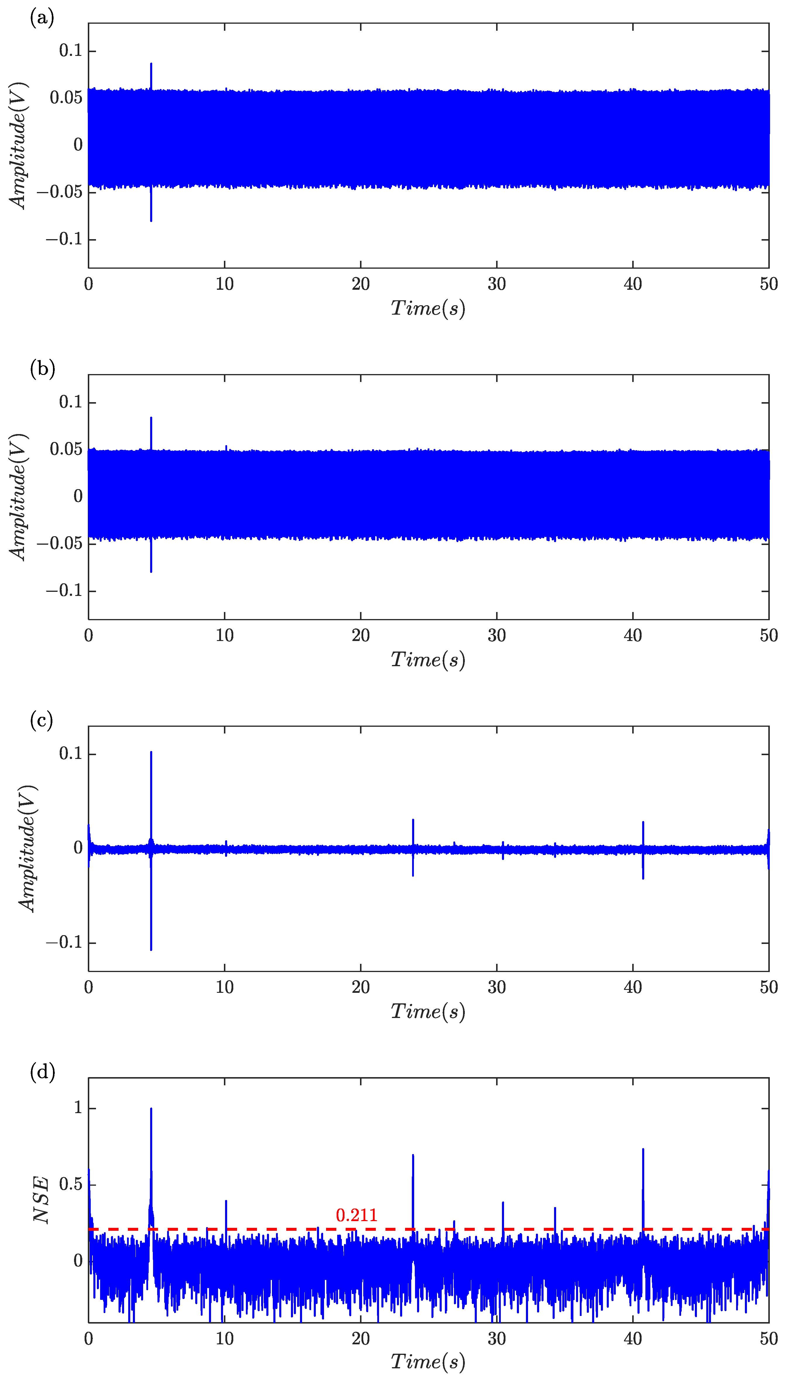
2.1. Signal Pre-Processed
2.2. Normalized Segmentation Entropy Detection
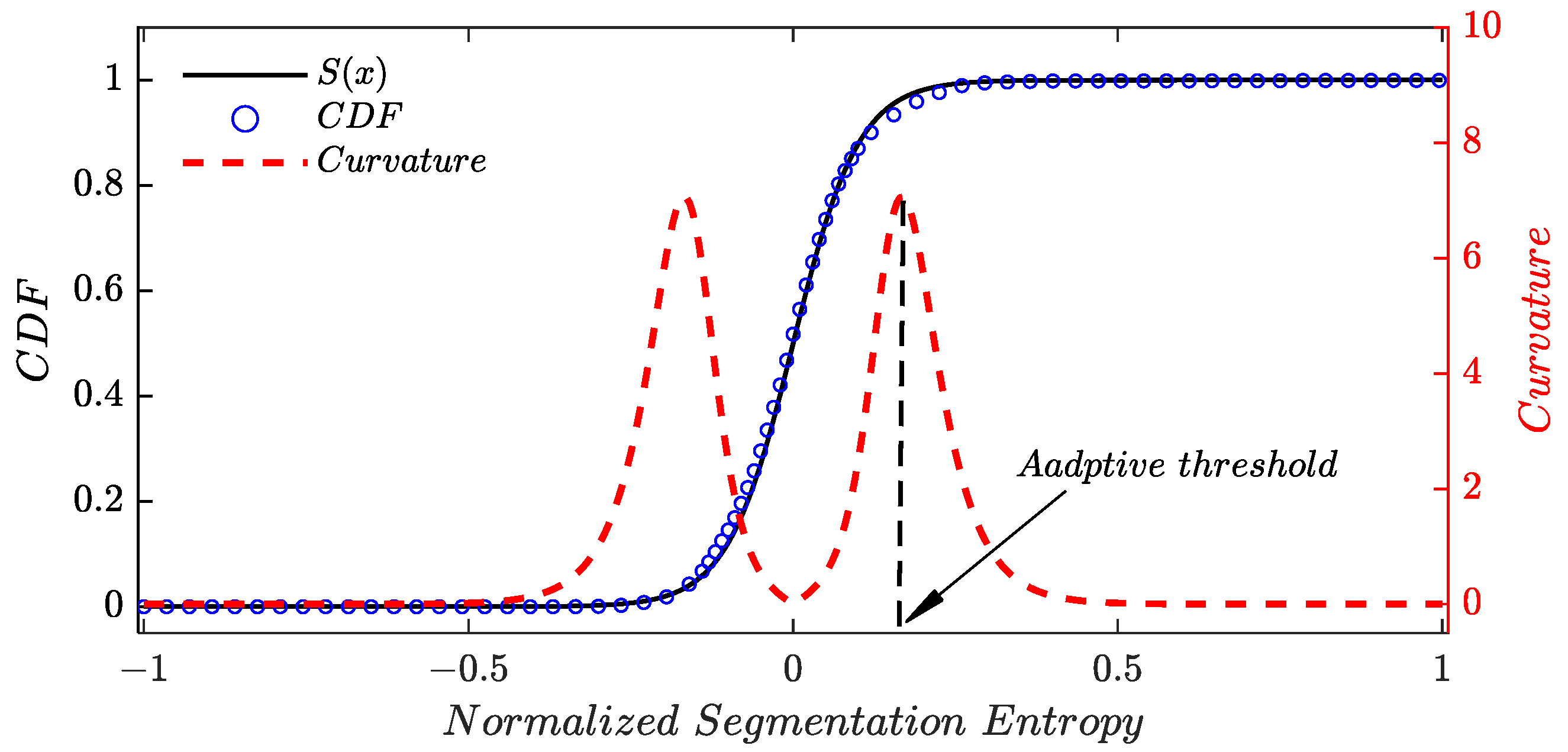
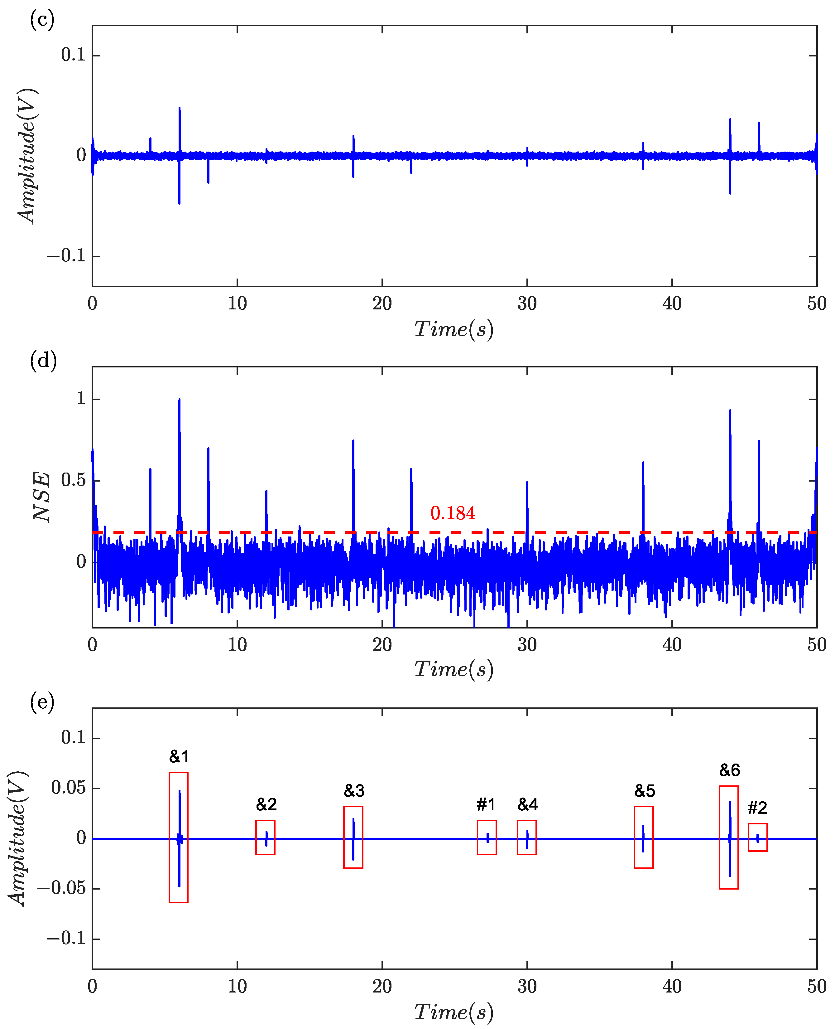
2.3. Adaptive Threshold Determination and Segmentation
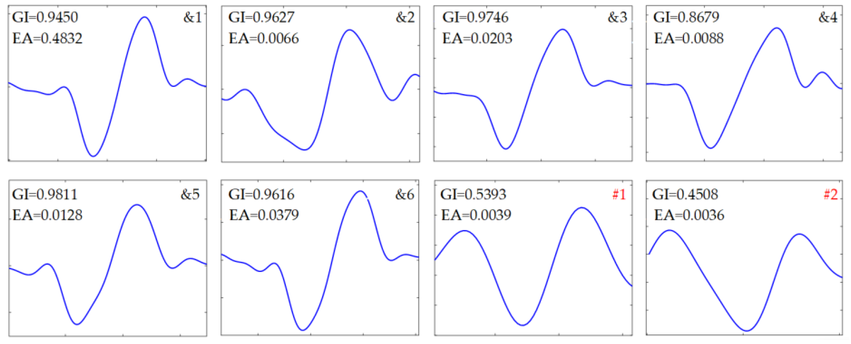
2.4. Identification and Counting of Debris Signal
- (1)
- Index of time sequence. Although the magnitudes of debris signals may vary, their waveforms typically exhibit a consistent pattern, wherein the former half is situated below the horizontal axis and the latter half is predominantly positive, as illustrated in Figure 2. Assuming the presence of non-zero blocks covering L elements, denoted as ∆ = {∆0, ∆1, …, ∆L−1}, the time sequence index β can be defined as
- (2)
- Index of zero point. Another distinctive characteristic of debris signals is the presence of a singular zero-crossing point between Lm and Ln. If multiple zero-crossings emerge within this interval, it suggests fluctuations within the acquired samples, a condition inconsistent with the sinusoidal pulse-like nature. Consequently, such occurrences warrant classification of the data block as a non-debris signal. An index in consideration of the zero point can be defined as
- (3)
- Index of edge feature. A high entropy may occasionally occur in noise-only parts that contain outliers; therefore, the corresponding samples would be retained for further processing. However, the segmentation entropy drops rapidly once the outliers are no longer covered by the data window. As a result, residual noises typically have a sharp decrease at the edges of the data block, resulting in a much shorter duration of data edges compared to that of debris signals. Based on the characteristics of debris signals, the data edge, extending from the peaks to the end points, typically persists for a duration of at least Ω samples. Although the weaker edge features may be susceptible to elimination during noise reduction or threshold segmentation processes, the duration of data block edges remains a valuable feature for discriminating against spurious debris signals. An indicator based on the edge feature of the data block can be defined as
- (4)
- Index of offset feature. Since the induced voltages generated by debris hold a symmetrical pattern, the samples below the zero line and the samples above the zero line would have the similar behavior. Therefore, the sum of maximum and minimum samples in data block would be very small. For residual noise and electric pulses, the bias would be easily observed because they can hardly possess a regularly symmetrical pattern. In order to get rid of the non-debris data, the indicator, describing the offset, is defined as
- (5)
- Index of energy feature. Although the most of non-target data blocks can be excluded by the former index, there are a few of noise samples that can still meet the requirement. For example, a series of consecutive low frequency noises may contain a sub-sequence, the pattern of which is very similar to a sine-like signal. In this case, the noise samples might be wrongly classified as a debris signal. To reduce the false discrimination rate, an index related to the energy feature is proposed
3. Simulation and Results
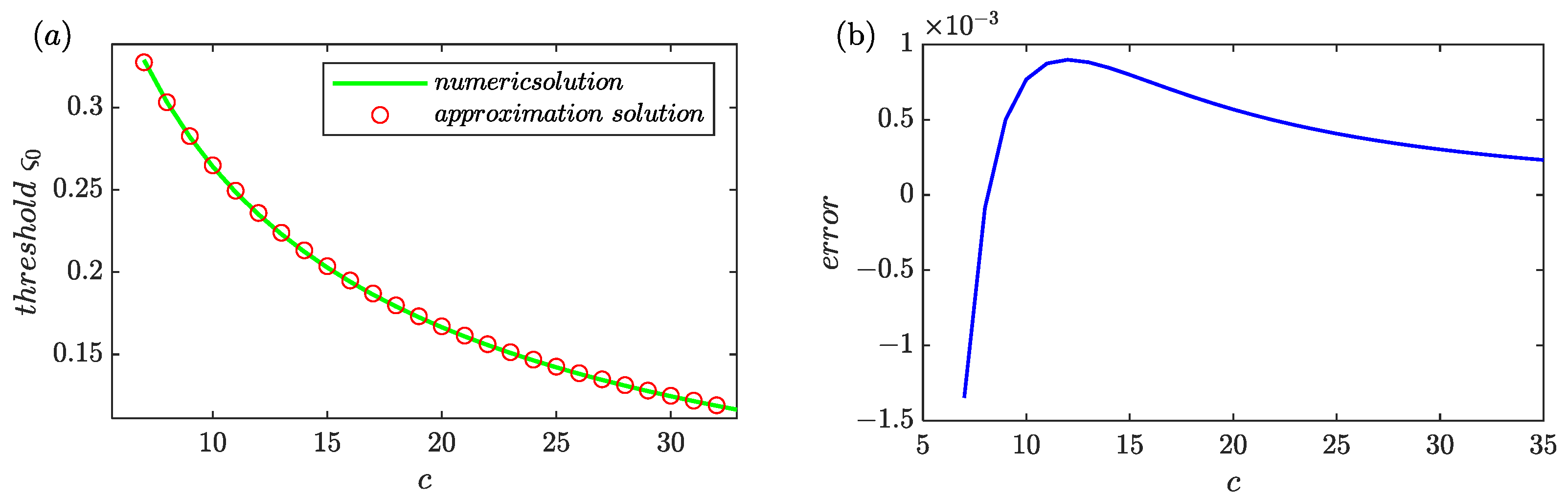
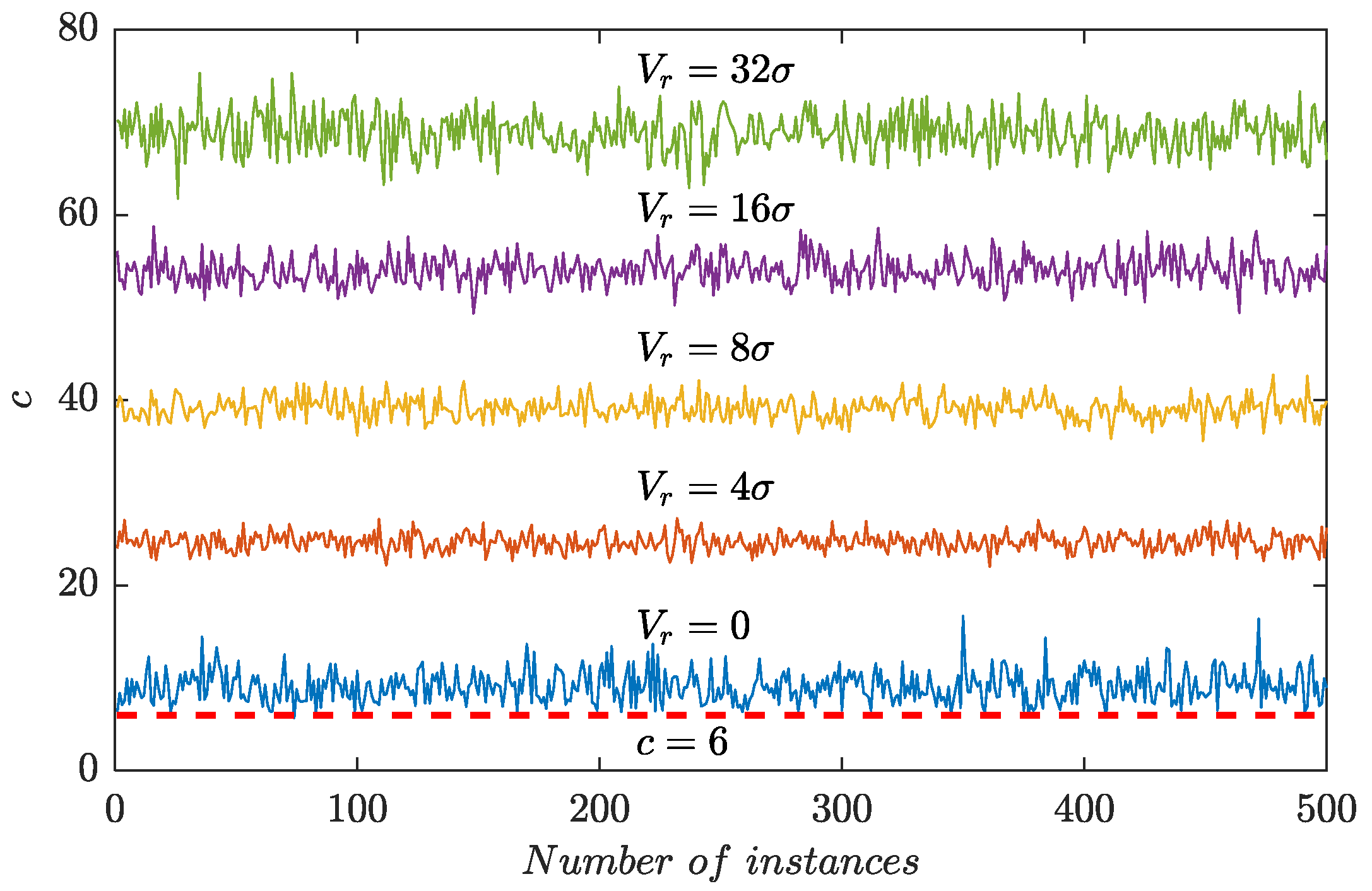
3.1. Verification of the Adaptive Threshold
3.2. Verification of the Feature Extraction and Identification
3.3. Verification of Robustness of the Proposed Algorithm
4. Experiments and Results
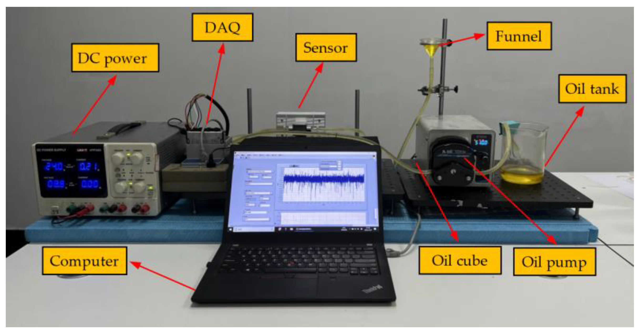
4.1. Experimental Settings and Data Acquisition
4.2. Experimental Results
4.3. Comparison and Discussion
5. Conclusions
Author Contributions
Funding
Informed Consent Statement
Data Availability Statement
Acknowledgments
Conflicts of Interest
Appendix A
Appendix B
References
- Su, L.; Shi, L.; Li, F.; Quan, J.; Zhao, S. Detection of weak pulse signal under chaotic noise based on fractional maximum correlation entropy Algorithm. In Journal of Physics: Conference Series; IOP Publishing: Bristol, UK, 2022; Volume 2290, p. 012075. [Google Scholar] [CrossRef]
- Petropoulos, P.; Ibsen, M.; Ellis, A.; Richardson, D. Rectangular pulse generation based on pulse reshaping using a superstructure fiber bragg grating. J. Light. Technol. 2001, 19, 746. [Google Scholar] [CrossRef]
- Xiao, Z.; Du, L.; Jiang, Z. A 3 × 3 wear debris sensor array for real time lubricant oil conditioning monitoring using synchronized sampling. Mech. Syst. Signal Process. 2017, 83, 296–304. [Google Scholar]
- He, Y.; Hu, M.; Feng, K.; Jiang, Z. Bearing condition evaluation based on the shock pulse method and principal resonance analysis. IEEE Trans. Instrum. Meas. 2021, 70, 1–12. [Google Scholar] [CrossRef]
- Mouritz, A.P.; Townsend, C.; Khan, M.Z.S. Non-destructive detection of fatigue damage in thick composites by pulse-echo ultrasonics. Compos. Sci. Technol. 2000, 60, 23–32. [Google Scholar] [CrossRef]
- Hong, W.; Li, T.; Wang, S.; Zhou, Z. A general framework for aliasing corrections of inductive oil debris detection based on artificial neural networks. IEEE Sens. J. 2020, 20, 10724–10732. [Google Scholar] [CrossRef]
- Bai, C.; Kan, X.; Yang, Y.; Yu, S.; Xu, Z.; Zhang, H.; Li, W. Dual-channel Metal Debris Signal Differential Detection Based on Frequency Division Multiplexing. IEEE Sens. J. 2024. early access. [Google Scholar]
- Du, L.; Zhe, J. A high throughput inductive pulse sensor for online oil debris monitoring. Tribol. Int. 2011, 44, 175–179. [Google Scholar] [CrossRef]
- Han, W.; Mu, X.; Liu, Y.; Wang, X.; Li, W.; Bai, C.; Zhang, H. A Critical Review of On-Line Oil Wear Debris Particle Detection Sensors. J. Mar. Sci. Eng. 2023, 11, 2363. [Google Scholar] [CrossRef]
- Zhang, H.; Zhang, Z.; Zhao, X.; Li, H.; Li, W.; Wang, C.; Bai, C.; Hu, S. An LC resonance-based sensor for multi-contaminant detection in oil fluids. IEEE Sens. J. 2024. early access. [Google Scholar]
- Wei, H.; Wenjian, C.; Shaoping, W.; Tomovic, M.M. Mechanical wear debris feature, detection, and diagnosis: A review. Chin. J. Aeronaut. 2018, 31, 867–882. [Google Scholar]
- Zhang, H.; Ma, L.; Shi, H.; Xie, Y.; Wang, C. A Method for Estimating the Composition and Size of Wear Debris in Lubricating Oil Based on the Joint Observation of Inductance and Resistance Signals: Theoretical Modeling and Experimental Verification. IEEE Trans. Instrum. Meas. 2022, 71, 1–9. [Google Scholar] [CrossRef]
- Hong, W.; Wang, S.; Tomovic, M.M.; Liu, H.; Wang, X. A new debris sensor based on dual excitation sources for online debris monitoring. Meas. Sci. Technol. 2015, 26, 095101. [Google Scholar] [CrossRef]
- Feng, S.; Yang, L.; Qiu, G.; Luo, J.; Li, R.; Mao, J. An inductive debris sensor based on a high-gradient magnetic field. IEEE Sens. J. 2019, 19, 2879–2886. [Google Scholar] [CrossRef]
- Hong, W.; Wang, S.; Liu, H.; Tomovic, M.M.; Chao, Z. A hybrid method based on band pass filter and correlation algorithm to improve debris sensor capacity. Mech. Syst. Signal Process. 2017, 82, 1–12. [Google Scholar] [CrossRef]
- Hong, H.; Liang, M. A fractional calculus technique for on-line detection of oil debris. Meas. Sci. Technol. 2008, 19, 055703. [Google Scholar] [CrossRef]
- Luo, J.; Li, J.; Wang, X.; Feng, S. An Inductive Sensor Based Multi-Least-Mean-Square Adaptive Weighting Filtering for Debris Feature Extraction. IEEE Trans. Ind. Electron. 2022, 70, 3115–3125. [Google Scholar] [CrossRef]
- Luo, J.; Xie, Z.; Xie, M. Frequency estimation of the weighted real tones or resolved multiple tones by iterative interpolation DFT algorithm. Digit. Signal Process. 2015, 41, 118–129. [Google Scholar] [CrossRef]
- Luo, J.; Xie, M. Phase difference methods based on asymmetric windows. Mech. Syst. Signal Process. 2015, 54, 52–67. [Google Scholar] [CrossRef]
- Jia, L.; Lei, L. A hybrid genetic algorithm based on information entropy and game theory. IEEE Access 2020, 8, 36602–36611. [Google Scholar]
- Osamy, W.; Salim, A.; Khedr, M.A. An information entropy based-clustering algorithm for heterogeneous wireless sensor networks. Wirel. Netw. 2020, 26, 1869–1886. [Google Scholar] [CrossRef]
- Ting, Y.; Hong, L.; Xiao, Z. Noise smoothing for structural vibration test signals using an improved wavelet thresholding technique. Sensors 2012, 12, 11205–11220. [Google Scholar]
- Bing, Y.; Nan, C.; Tian, Z. A Novel Signature Extracting Approach for Inductive Oil Debris Sensors based on Symplectic Geometry Mode Decomposition. Measurement 2021, 185, 11005. [Google Scholar]
- Fan, X.; Liang, M.; Yeap, T. A Joint Time-Invariant Wavelet Transform and Kurtosis Approach to the Improvement of In-Line Oil Debris Sensor Capability. Smart Mater. Struct. 2009, 18, 085010. [Google Scholar] [CrossRef]


| Order | Steps and Algorithms |
|---|---|
| 1 | Induced voltages acquisition and data conversation |
| 2 | Elimination of high frequency noise using low-pass filtering and harmonics suppression using parameter estimation |
| 3 | Calculation of the normalized segmentation entropy using Equation (2) |
| 4 | Determination of the adaptive threshold using Equation (5) and segmentation of the suspected characteristic signal with the adaptive threshold |
| 5 | Calculation of the five indicators as well as the global threshold and performing the debris signal identification with β = 1, ζ = 1, ξ > 0.7, γ > 0.7, η > 0.7 and GT > 0.6 |
| 6 | Amplitude classification and counting |
| Order | ξ | γ | η | GI |
|---|---|---|---|---|
| &1 | 0.9963 | 1.0000 | 0.9485 | 0.9450 |
| &2 | 0.9971 | 1.0000 | 0.9656 | 0.9627 |
| &3 | 0.9746 | 1.0000 | 1.0000 | 0.9746 |
| &4 | 0.9102 | 0.9643 | 0.9889 | 0.8679 |
| &5 | 0.9919 | 1.0000 | 0.9869 | 0.9811 |
| &6 | 0.9911 | 1.0000 | 0.9702 | 0.9616 |
| #1 | 0.8208 | 0.8333 | 0.7885 | 0.5393 |
| #2 | 0.9451 | 0.7931 | 0.6014 | 0.4508 |
| Order | DR | MV | STD (×10−4) |
|---|---|---|---|
| &1 | 100% | 0.0475 | 8.763 |
| &2 | 82% | 0.0059 | 6.524 |
| &3 | 100% | 0.0189 | 5.668 |
| &4 | 91% | 0.0078 | 7.710 |
| &5 | 99% | 0.0116 | 5.521 |
| &6 | 100% | 0.0379 | 8.399 |
| Order | ξ | γ | η | GI | EA |
|---|---|---|---|---|---|
| I | 0.9473 | 1.0000 | 0.7786 | 0.7375 | 0.0043 |
| II | 0.8202 | 0.7917 | 0.8806 | 0.5718 | 0.0033 |
| III | 0.9658 | 0.8889 | 0.6878 | 0.5904 | 0.0038 |
| IV | 0.9048 | 1.0000 | 0.8639 | 0.7817 | 0.0031 |
| V | 0.8183 | 1.0000 | 0.9931 | 0.8126 | 0.0041 |
| VI | 0.8678 | 1.0000 | 0.9823 | 0.8524 | 0.0038 |
| VII | 0.8079 | 1.0000 | 0.8173 | 0.6604 | 0.0035 |
| X | 0.8132 | 0.7895 | 0.8565 | 0.5499 | 0.0040 |
| IX | 0.9485 | 1.0000 | 0.7929 | 0.7520 | 0.0040 |
| Order | ξ | γ | η | GI | EA |
|---|---|---|---|---|---|
| &1 | 0.9776 | 1.0000 | 0.9403 | 0.9192 | 0.1049 |
| &2 | 0.9859 | 0.9091 | 1.0000 | 0.8963 | 0.0077 |
| &3 | 0.9657 | 1.0000 | 1.0000 | 0.9657 | 0.0297 |
| &4 | 0.8393 | 0.9615 | 1.0000 | 0.8071 | 0.0056 |
| &5 | 0.7779 | 1.0000 | 1.0000 | 0.7779 | 0.0089 |
| &6 | 0.7887 | 1.0000 | 0.9941 | 0.7841 | 0.0071 |
| &7 | 0.9395 | 1.0000 | 0.9893 | 0.9295 | 0.0299 |
Disclaimer/Publisher’s Note: The statements, opinions and data contained in all publications are solely those of the individual author(s) and contributor(s) and not of MDPI and/or the editor(s). MDPI and/or the editor(s) disclaim responsibility for any injury to people or property resulting from any ideas, methods, instructions or products referred to in the content. |
© 2024 by the authors. Licensee MDPI, Basel, Switzerland. This article is an open access article distributed under the terms and conditions of the Creative Commons Attribution (CC BY) license (https://creativecommons.org/licenses/by/4.0/).
Share and Cite
Yang, B.; Liu, W.; Lu, S.; Luo, J. Feature Extraction of Lubricating Oil Debris Signal Based on Segmentation Entropy with an Adaptive Threshold. Sensors 2024, 24, 1380. https://doi.org/10.3390/s24051380
Yang B, Liu W, Lu S, Luo J. Feature Extraction of Lubricating Oil Debris Signal Based on Segmentation Entropy with an Adaptive Threshold. Sensors. 2024; 24(5):1380. https://doi.org/10.3390/s24051380
Chicago/Turabian StyleYang, Baojun, Wei Liu, Sheng Lu, and Jiufei Luo. 2024. "Feature Extraction of Lubricating Oil Debris Signal Based on Segmentation Entropy with an Adaptive Threshold" Sensors 24, no. 5: 1380. https://doi.org/10.3390/s24051380
APA StyleYang, B., Liu, W., Lu, S., & Luo, J. (2024). Feature Extraction of Lubricating Oil Debris Signal Based on Segmentation Entropy with an Adaptive Threshold. Sensors, 24(5), 1380. https://doi.org/10.3390/s24051380