
Multispectral Light Detection and Ranging Technology and Applications: A Review


Abstract
:1. Introduction
1.1. Paper’s Contribution
- What is the historical evolution, current status, and prospective future of MSL technology?
- What advantages do MSL data offer in comparison to multispectral images as well as monochromatic LiDAR data?
- What categorizations exist for MSL data, and what are the inherent potentials and challenges associated with each?
- Are there established benchmark datasets available for MSL?
- What is the scope of the application of MSL within the fields of remote sensing and photogrammetry?
- What are the prospective benefits, opportunities, and challenges linked with MSL technology?
1.2. Literature Search Strategy
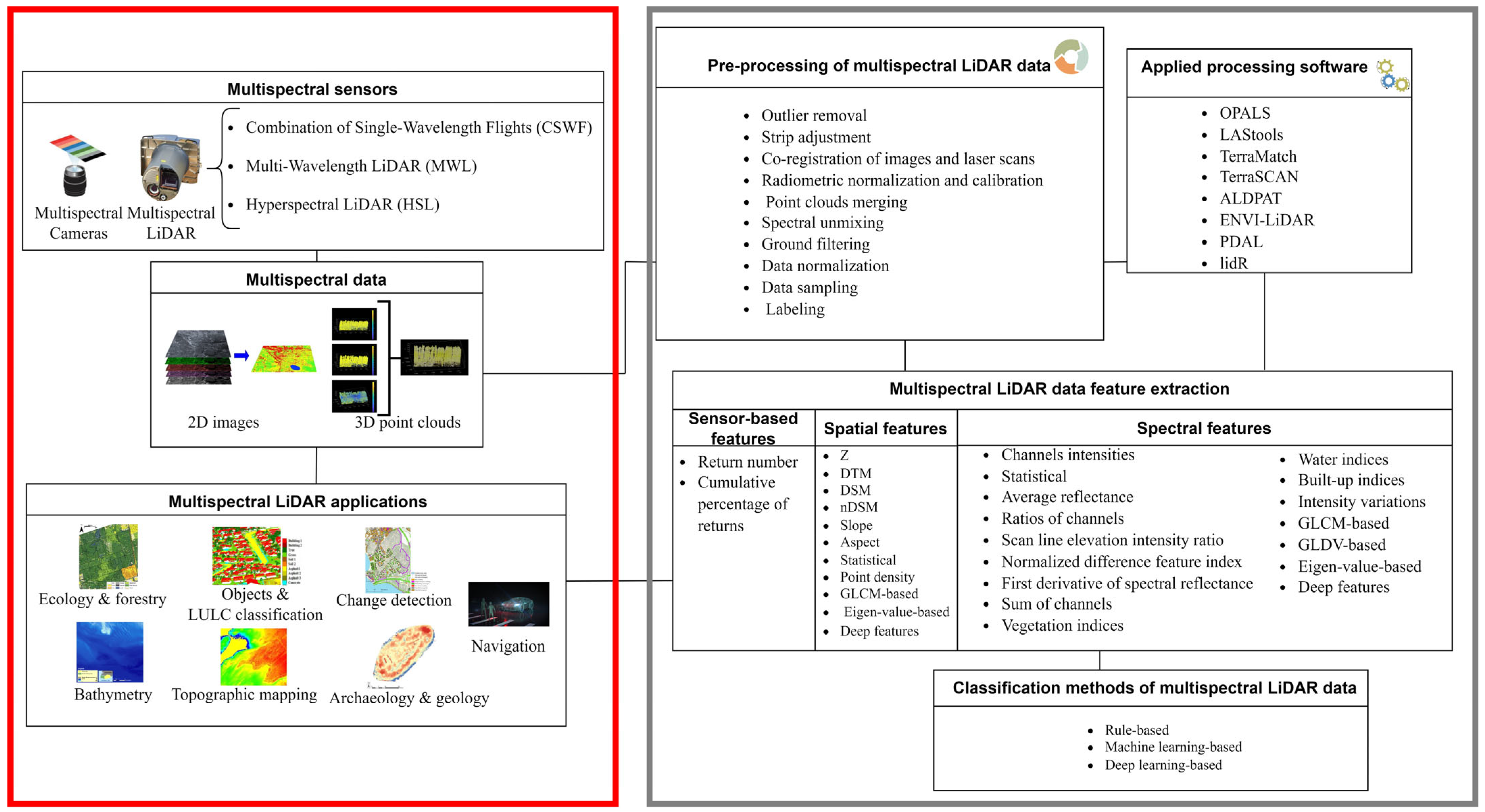
2. Multispectral Sensors
2.1. Multispectral Passive Sensors
2.2. Multispectral Laser Systems
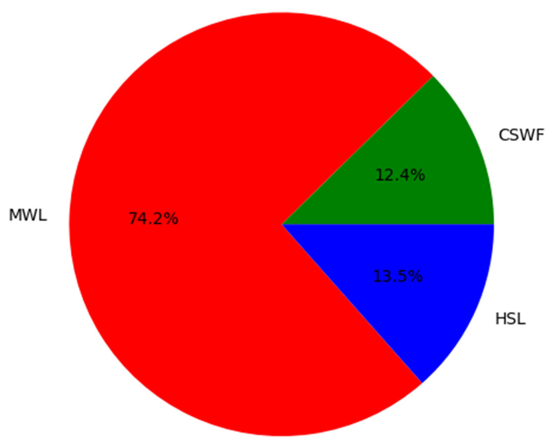
2.2.1. Combination of Single-Wavelength Flights (CSWF)
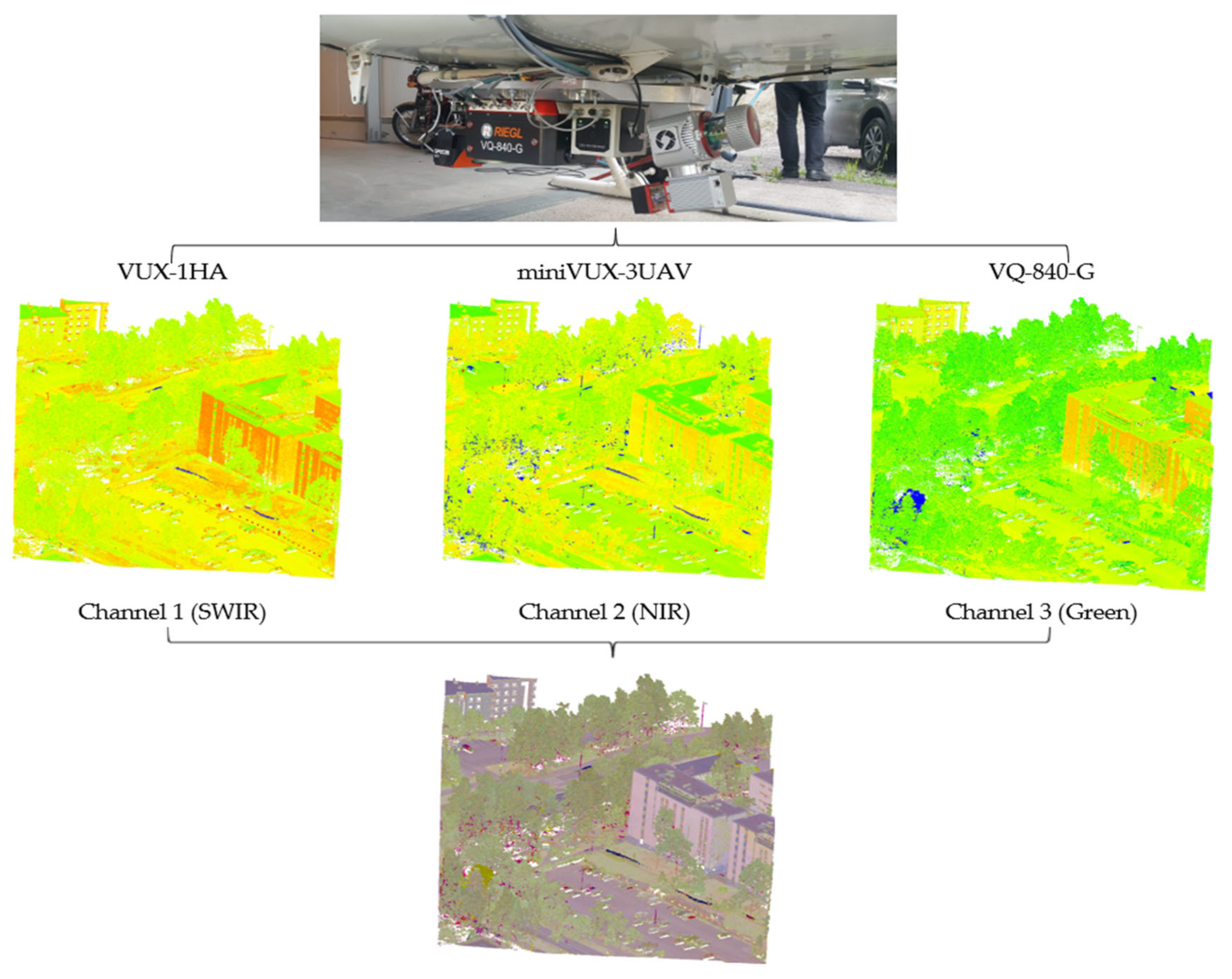
2.2.2. Multi-Wavelength LiDAR (MWL)

| LiDAR Sensor | Producer | Wavelength [nm] | Main Application | Beam Divergence [mrad] | Looking Angle [°] | PRF [kHz] | PD [points/m2] |
|---|---|---|---|---|---|---|---|
| Optech Titan, A | Teledyne Optech | C1: 1550 C2: 1064 C3: 532 | Multi-purpose | C1: 0.35 C2: 0.35 C3: 0.7 | C1: 3.5 C2: 0 C3: 7 | 900 | Bathymetry: >5 pts/m2 Topography: >45 pts/m2 |
| HeliALS-TW, A | FGI | C1: 1550 C2: 905 C3: 532 | Forest inventory | C1: 0.5 C2: 0.5 × 1.6 C3: 1 | C1: 360 C2: 120 C3: 28 × 40 | C1: 1017 C2: 300 C3: 200 | C1: 1400 C2: 500 C3: 1600 |
| HawkEye-5, A [82] | Leica | C1: 515 C2: 515 C3: 1064 | Deep and shallow bathymetry & topography | C1: 7.5 C2: 4.75 C3: 0.5 | ±14 front/back ±20 left/right | C1:40 C2: 200 C3: 500,000 | C1: 1 C2: 5 C3: 12 |
| VQ-880-GH, A [83] | RIEGL | C1: 532 C2: 1064 | Deep and shallow bathymetry & topography | 0.7–2 | 40 | C1: 700 C2: 279 | NA |
| CZMIL Supernova, A [84] | Optech | C1: 532 C2: 532 C3: 1064 | Deep and shallow bathymetry & topography | 7 | 40 | C1:30 C2: 210 C3: 240 | Shallow water ≤ 8 Deep water ≥ 1 |
| VQ-1560i-DW, A | RIEGL | C1: 532 C2: 1064 | Agriculture & forestry, bathymetry | C1: 0.7–2 C2: 0.18–0.25 | 14 | 1000 | 2–60 |
| Chiroptera4X, A [85] | Leica | C1: 532 C2: 1064 | Bathymetry & topography | ~3 | ±14 front/back, ±20 left/right | 140 500 | Bathymetry: >5 Topography: >10 |
| DWEL, T | Boston University | C1: 1064 C2: 1548 | Forest inventory | 1.25, 2.5, or 5 | ±119 front/back ±119 left/right | 20 | NA |
| BAM, T | BAM | C1: 670 C2: 810 C3: 980 C4: 1930 | Inspection of building surfaces | NA | 30 | 10,000 | NA |
| MWCL, T | Wuhan University | C1:555 C2: 670 C3: 700 C4: 780 | Vegetation mapping | C1: 0.3 × 0.6 C2: 0.3 × 0.6 C3: 0.2 × 0.6 C4: 0.2 × 0.6 | 25 | 0.8 | NA |
2.2.3. Hyperspectral LiDAR (HSL)
2.2.4. Historical Development of Multispectral LiDAR
3. Multispectral LiDAR Data
MSL Benchmark Datasets
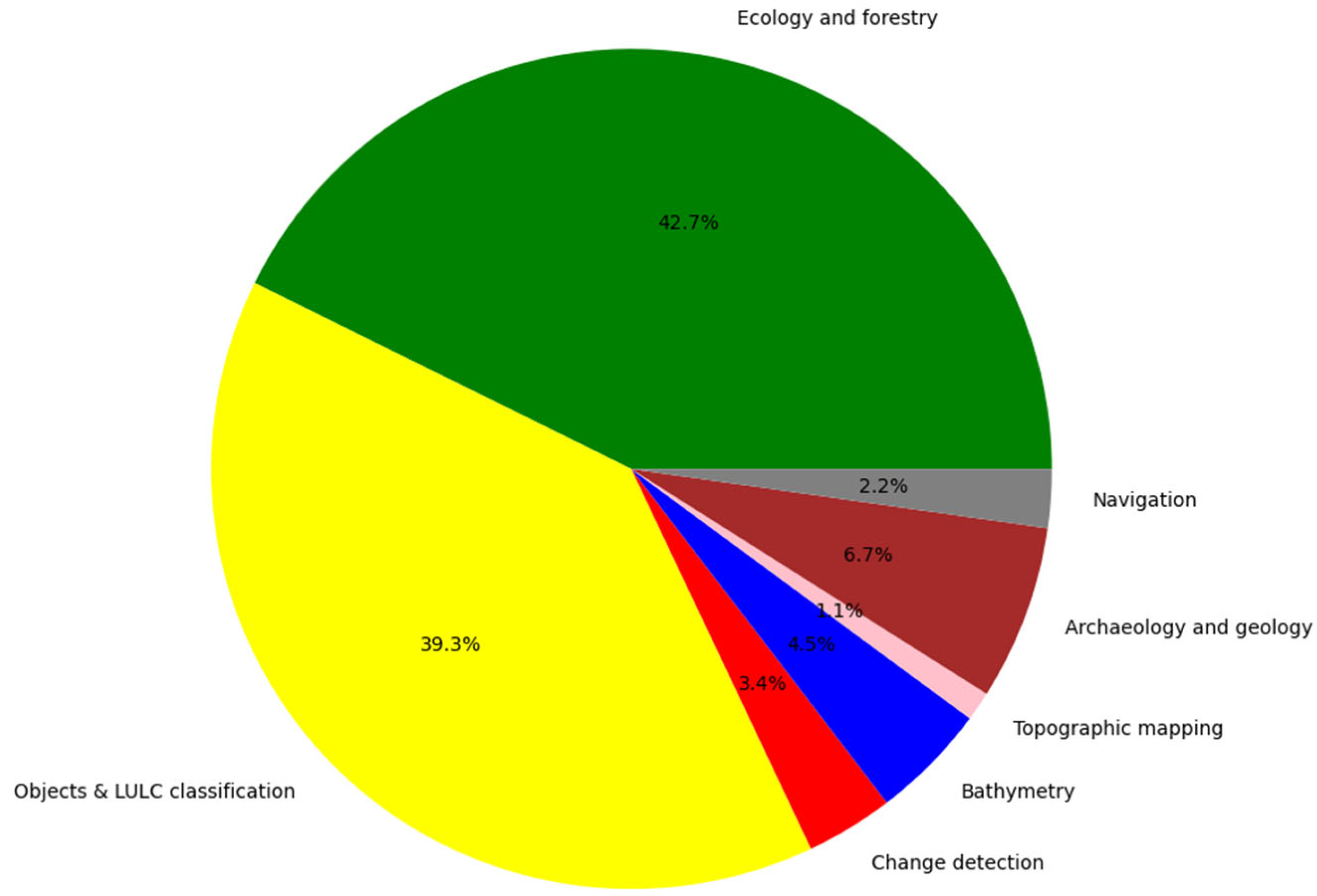
4. Multispectral LiDAR Applications
4.1. Ecology and Forestry
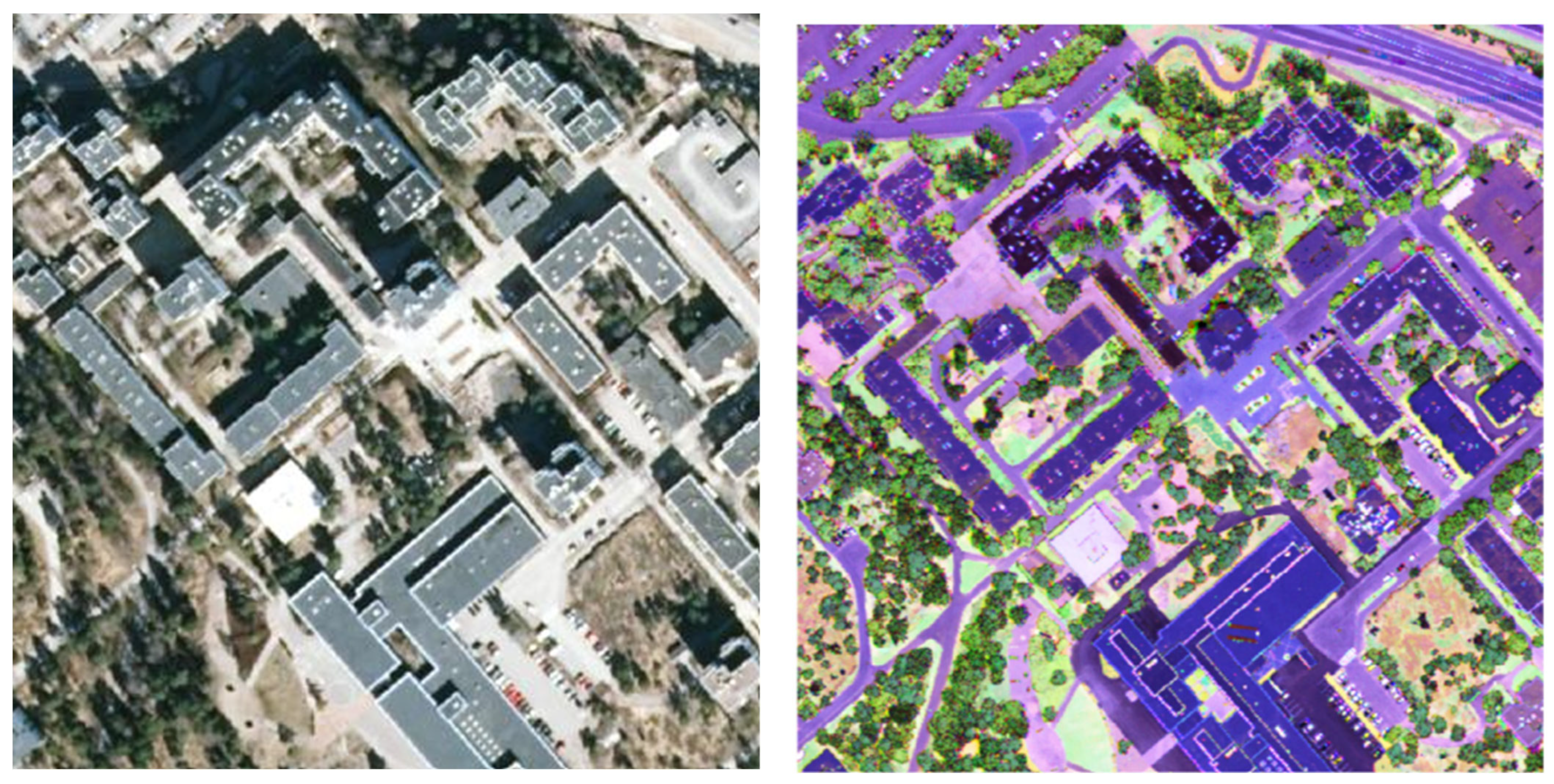
4.2. Objects and LULC Classification
4.3. Change Detection
4.4. Bathymetry
4.5. Topographic Mapping
4.6. Archaeology and Geology
4.7. Navigation
5. Discussion
6. Conclusions
- The majority of MSL/HSL systems are designed for experimental purposes. Notably, there is currently no commercially available HSL system at the moments. Consequently, there is a need to introduce new MSL/HSL systems to the market.
- Due to the promising capabilities of NASA’s GEDI spaceborne LiDAR (launched in late 2018) in canopy height and aboveground biomass estimation, satellite-based MSL can be also anticipated in the near future [135].
- Given that spectral information constitutes the primary advantage of MSL technology over monochromatic LiDAR, there is an increased demand for precise radiometric calibration [136]. Therefore, it is worthwhile to consider the incorporation of a radiometric calibration component in the design of the new generation of MSL/HSL systems.
- A notable limitation of Titan data is the presence of inhomogeneity within the point clouds, as significant discrepancies in the data between the across-track and along-track directions are visible [137]. Given that the 3-wavelength Optech Titan data are currently the most commonly utilized data in various studies, it becomes evident that there is a demand for the development and exploration of new commercial MSL/HSL systems with enhanced specifications in the near future. To address the mentioned issue and achieve a more uniform point spacing, upcoming MSL systems can consider either reducing the aircraft speed or increasing the scan frequency [137].
- Multispectral LiDAR instruments ought to be both cost-effective and compact in size, thereby facilitating their adoption into academic and industrial domains.
- The majority of SC-based HSL systems currently feature fewer than 10 spectral channels. Therefore, there is a need for the introduction of new HSL systems that offer a broader range of spectral information. Overcoming eye-safety issues is a primary consideration in this context.
- More attempts should be made for directly processing 3D MSL/HSL point clouds instead of considering rasterized data form.
- Benchmark datasets in MSL/HSL for scientific purposes, especially those with ground truth data, are still lacking.
- During recent years, forestry and LULC mapping have received by far the most attention from scholars. More studies are needed to be dedicated to the other mentioned applications of MSL, especially archaeology, navigation, and change detection.
- Multispectral laser scanning is expected to yield a broader spectrum of applications, such as extending to precision agriculture, disaster risk management, distinguishing pollution in environment, and detecting obscured targets [136].
- Increased attention should be directed towards thorough exploration of the potential opportunities of HSL systems.
Author Contributions
Funding
Institutional Review Board Statement
Informed Consent Statement
Data Availability Statement
Conflicts of Interest
Appendix A
| Publications | Data Sources | Application | Feature(s) Type | Method(s) |
|---|---|---|---|---|
| Hakula et al., 2023 [68] | HeliALS-TW | Tree species classification | Several geometric, radiometric and return type features | P Object-based RF |
| Rana et al., 2023 [114] | Optech Titan | Monitoring seedling stands | Geometric, intensities | P Linear regression |
| Axelsson et al., 2023 [138] | VQ-1560i-DW | Tree species classification and stem volumes estimation | Several geometric, radiometric and return type features | P LDA and k-nearest neighbors models |
| Shao al., 2023 [90] | AOTF-HSL | Persimmon tree components classification | Intensities, average reflectance, CI red edge, NDVI, NDRE | P RF, SVM, and backpropagation neural network methods |
| Xiao et al., 2022 [119] | Optech Titan | LULC classification | Z, intensity, and SVD-based and deep features | P Improved RandLA-Net |
| Tian et al., 2022 [110] | Designed HSL | Plant species classification | Deep features and vegetation indices | I VI-CNN |
| Zhang et al., 2022 [121] | Optech Titan | LULC classification | Deep | P MPT + network |
| Taher et al., 2022 [134] | Designed HSL | Autonomous vehicle perception | Intensities and geometric | I RF |
| Li et al., 2022 [139] | Optech Titan | LULC classification | Deep | P AGFP-Net |
| Mielczarek et al., 2022 [109] | VQ-1560i-DW | Invasive tree species identification | Statistical features of intensities, GNDVI | P Object-based RF, gradient boosting, Xgboost, and SAMME.R |
| Luo et al., 2022 [10] | Optech Titan | LULC classification | DSM, intensities, pNDVIs | P Decision tree |
| Sun et al., 2022 [44] | Designed HSL | Objects (manufacturing materials, plants and ore species) classification | Intensities | P Rule-based |
| Morsy et al., 2022 [8] | Optech Titan | LULC classification | Z, pNDVIs | P Rule-based |
| Lindberg et al., 2021 [99] | Optech Titan | Tree species classification | Mean and std of intensities | I LDA |
| Shao et al., 2021 [91] | AOTF-HSL | Wood-leaf separation | Intensity ratio, first derivative of spectral reflectance | P Rule-based |
| O. Ali et al., 2021 [132] | Optech Titan | DTM generation | Z and intensities | P Adaptive TIN, elevation threshold, progressive morphological algorithms, and maximum local slope |
| Shi et al., 2021 [122] | Optech Titan | LULC classification | Multi-scale statistical features and NDFIs | P SVM |
| Ghaseminik et al., 2021 [123] | Optech Titan | LULC classification | Intensity images, DTM, DSM, n DSM, slope, aspect, eigen value-based features, | I Object-based RF |
| Zhao et al., 2021 [140] | Optech Titan | LULC classification | Deep | P FR-GCNet |
| Jing et al., 2021 [141] | Optech Titan | LULC classification | Deep | P Squeeze-and-Excitation (SE) PointNet++ |
| Pan et al., 2020 [142] | Optech Titan | LULC classification | Deep | I CNN |
| Imangholiloo et al., 2020 [143] | Optech Titan | Forest inventory | CHM, pNDVI, intensities and its ratio and statistical features | I Object-based RF |
| Jiang et al., 2020 [92] | AOTF-HSL | Points cloud classification | Intensity ratios | P Rule-based classification |
| Huo & Lindberg, 2020 [111] | Optech Titan | Individual tree detection | Maximum height, point density, vegetation ratio, and average intensities | P Local height maximum filter and similarity maps |
| Matikainen et al., 2020 [55] | Combination of SPL100 and Optech Titan | LULC classification | Geometric-spectral statistical features, Geometric-spectral GLCM-based and GLDV-based textural features, pNDVI, brightness, pNDBI, intensity ratios | I Object-based RF |
| Maltamo et al., 2020 [113] | Optech Titan | Prediction of forest canopy fuel parameters | Geometric-spectral statistical features, echo class proportion, sum of intensities, ratio of two channels | I LDA and linear regression |
| Goodbody et al., 2020 [112] | Optech Titan | Forest inventory and diversity attribute modelling | Geometric-spectral statistical features, NDFI, sum of all channels, ratios of two channels and CVI | P RF |
| Li et al., 2020 [19] | Optech Titan | Buildings extraction | Deep | P Graph Geometric Moments (GGM) convolution |
| Jiang et al., 2020 [93] | AOTF-HSL | SLAM points cloud matching | Spectral ratio | P Iterative Closest Point (ICP) |
| Yan et al., 2020 [144] | Optech Titan | Predicting forest attributes | Geometric-spectral statistical features and pNDVIs | P RF |
| Junttila et al., 2019 [145] | Integration of FARO X330 and Trimble TX5 | Detecting tree infestation | Spectral statistical features and density bandwidth | P Regressions and linear discriminant analysis |
| Kukkonen al., 2019 [28] | Optech Titan | Tree species classification | Geometric statistical features, channel intensities, sum of two channels, sum of all channels, ratios of two channels | I k-nearest neighbors |
| Jiang al., 2019 [22] | AOTF-HSL | Vegetation red edge parameters extraction | Intensities | P First-order differential of the spectral reflectance |
| Shao et al., 2019 [87] | AOTF-HSL | Coal/rock classification | Intensities | P Naive Bayes, logistic regression, and SVM |
| Pan et al., 2019 [124] | Optech Titan | LULC classification | Deep, intensities, GDVI, GRVI, GNDVI, MNDWI, Geometric-spectral GLCM | I DBM-based deep feature extraction, PCA-based and RF-based low level feature selection, SVM |
| Wang and Gu, 2019 [146] | Optech Titan | LULC classification | Geometric-spectral eigen values | P Tensor manifold discriminant embedding and SVM |
| Pilarska et al., 2019 [147] | VQ-1560i-DW | Urban tree classification | Spectral statistical features and pNDVI | P SVM |
| Kukkonen al., 2019 [12] | Optech Titan | Tree species classification and predicting species’ volume proportions | Intensity, geometric-spectral statistical features, channels ratios, binary sum of two channels, and density | I LDA model |
| Matikainen et al., 2019 [103] | Optech Titan | Change detection | DSM, intensities, pNDVI, and NDBI | I Object-based RF and rule-based classification |
| Shao et al., 2019 [94] | AOTF-HSL | Architectural heritage preservation | Intensities | P Naive Bayes and SVM |
| Junttila et al., 2018 [49] | Integration of Leica HDS6100, FARO S120 and FARO X330 | Estimating leaf water content | Spectral statistical features, normalized difference indices and spectral ratios | P Simple linear regression |
| Karila et al., 2018 [118] | Optech Titan | LULC classification and road detection | Spectral statistical features, intensity ratios, GLCM homogeneity, ratios of two channels, PNDVI, and NDBI) and DSM features (std, GLCM homogeneity, and quartiles difference) | I Object-based RF |
| Ekhtari et al., 2018 [7] | Optech Titan | LULC classification | nDSM and intensities | P SVM and rule-based classification |
| Dai et al., 2018 [17] | Optech Titan | Individual tree detection | Geometric features and intensities | P Mean shift segmentation and SVM |
| Pilarska, 2018 [148] | VQ-1560i-DW | LULC classification and road detection | nDSM, intensities, and GNDVI | I Rule-based classification |
| Chen et al., 2018 [116] | Optech Titan | Quantifying the carbon storage in urban trees | nDSM, intensity images, pNDVI, and pNDWI | I SVM, watershed segmentation, and allometry-based linear regression |
| Huo et al., 2018 [149] | Optech Titan | LULC classification | Intensities, nDSM, pNDVI, morphological profiles, and a novel hierarchical morphological profiles | I SVM |
| Axelsson et al., 2018 [150] | Optech Titan | Tree species classification | Statistical features of heights and intensities | P LDA model |
| Dalponte et al., 2018 [11] | Optech Titan | Predicting forest stand characteristics | Statistical features of heights and intensities | P Ordinary least squares regression |
| Yan et al., 2018 [130] | Optech Titan | Water surface mapping | Elevation, elevation variation, intensity, intensity variation, number of returns and NDFIs | P maximum likelihood |
| Kaszczuk et al., 2018 [151] | MSL | Plants condition analysis | NA | NA |
| Goraj et al., 2018 [131] | VQ-1560i-DW | Identifying hydromorphological indicators | Statistical features of intensities, and NDVI | I Regression |
| Chen, 2018 [152] | Optech Titan | LULC classification | Deep | I 3D CNN |
| Matikainen et al., 2017 [16] | Optech Titan | LULC classification | 41 features based on DSM, DTM, and intensityimages of three channels | I Object-based RF |
| Yu et al., 2017 [153] | Optech Titan | Tree species classification | 145 features based on Z, density, number of returns, 2D and 3D convex hull, spatial statistical features | P Object-based RF |
| Morsy et al., 2017 [154] | Optech Titan | LULC classification | Z, and pNDVIs | P Gaussian decomposition-based clustering |
| Karila et al., 2017 [18] | Optech Titan | Road mapping | Mean, std, quantiles and ratios of channels, pNDVI, DSM differences | I Object-based RF |
| Morsy et al., 2017 [129] | Optech Titan | Land/water classification | Elevation difference and roughness, intensity coefficient of variation (ICOV) and intensity density (ID), point density (PD) and multiple returns (MR) | P Rule-based classification |
| Matikainen et al., 2017 [126] | Optech Titan | LULC classification, road mapping, and change detection | DSM, DTM, intensity images | I Object-based RF |
| Morsy et al., 2017 [97] | Optech Titan | LULC classification | Z/DSM and three pNDVIs | P Maximum likelihood and rule-based classification |
| Budei et al., 2017 [13] | Optech Titan | Tree species classification | pNDVIs, intensities, CHM | I RF |
| Teo and Wu, 2017 [14] | Optech Titan | LULC classification | nDSM, intensities, NDFIs, curvatures | I Object-based SVM |
| Morsy et al., 2016 [155] | Optech Titan | LULC classification | NDWI, pNDWI, MNDWI | P Rule-based classification |
| Ahokas et al., 2016 [137] | Optech Titan | Tree species and LULC classification | DSM and several statistical features of intensity images | I Object-based RF |
| Hopkinson et al., 2016 [77] | Integration of Aquarius and Orion, Gemini, and Optech Titan | Forest land surface classification and vertical foliage partitioning | Intensities | I Minimum distance, maximum likelihood and parallelepiped classification routines |
| Nabucet et al., 2016 [156] | Optech Titan | Urban vegetation mapping | CHM and NDFI | I Object-based rule-based classification |
| Bakuła et al., 2016 [157] | Optech Titan | LULC classification | nDSM, intensities, morphological granulometric features | I Integration of maximum likelihood and rule-based classification |
| Fernandez-Diaz et al., 2016 [128] | Optech Titan | LULC classification, bathymetry mapping, thick vegetation canopies mapping | DSM and intensities | I Mahalanobis distance and the maximum likelihood |
| ZOU et al., 2016 [158] | Optech Titan | LULC classification | pNDVI, elevation difference ratio_green, ratio_count | I Object-based rule-based classification |
| Junttila et al., 2016 [115] | Integration of FARO X330 and Leica HDS6100 | Measuring leaf water content | Spectral statistical features, ratios of intensities, and NDFI | P Simple linear regression |
| Morsy et al., 2016 [9] | Optech Titan | LULC classification | DSM and intensities | I Maximum Likelihood |
| Matikainen et al., 2016 [125] | Optech Titan | Change detection | Spectral statistical features, intensity ratios, NDVI, DSM and its statistical features, homogeneity of DSM | I Object-based RF |
| Miller et al., 2016 [159] | Optech Titan | LULC classification | Height, return number, intensities, pNDVI | I Maximum likelihood |
| Hakala et al., 2015 [160] | Designed HSL | Monitoring pine chlorophyll content | MCARI750, MSR2, SR6 and NDVI | P Regression |
| Bakuła, 2015 [161] | Optech Titan | LULC classification | nDSM, intensities | P Terrasolid software |
| Shi et al., 2015 [162] | MWCL | LULC classification | Vegetation indices (NDVI, GNDVI, and SRPI) | P SVM |
| Junttila et al., 2015 [163] | Full waveform HSL | Trees drought detection | Spectral statistical features, NDVI, and a modified water index | P Rule-based classification |
| Lindberg et al., 2015 [74] | Integration of VQ-820-G and VQ-580, VQ-820-G and VQ-480i | Tree species classification | nDSM and maximum reflectance of first return for each wavelength | I Rule-based classification |
| Wichmann et al., 2015 [120] | Optech Titan | LULC classification | Intensities and pNDVI | P Mahalanobis distance |
| Gong et al., 2015 [78] | Wuhan MSL | LULC classification | Intensities | I SVM |
| Hartzell et al., 2014 [133] | Integration of RIEGL VZ-400 TLS and Nikon D700 camera | Rock type identification | Intensities | I Minimum distance |
| Wallace et al., 2014 [43] | TCSPC | Recovery of arboreal parameters | Intensities, NDVI, and PRI | I Reversible jump Markov chain Monte Carlo |
| Gaulton et al., 2013 [164] | SALCA | Estimating vegetation moisture content | NDFIs, ratios of intensities, NDWI and moisture stress index | P Major axis regression |
| Briese et al., 2013 [73] | Integration of VQ-820-G and VQ-580, VQ-820-G and VQ-480i | Archaeological prospection | Intensities | I Visual interpretation |
| Wang et al., 2013 [54] | Pegasus and Q680i | LULC classification | Z, echo width, and intensities | I SVM |
| Wallace et al., 2012 [80] | SELEX GALILEO | Forest canopy parameter estimation | NDVI and PRI | I MCMC and RJMCMC simulation |
| Woodhouse et al., 2011 [79] | Designed MSL | Measuring plant physiology | Z, PRI and NDVI | P TREEGROW model |
| Gaulton et al., 2010 [70] | SALCA | Measurement of canopy parameters | Intensities | P Rule-based |
| Wehr et al., 2006 [69] | BAM | Inspection of building surfaces | Intensities, NDVI, NDMI | I Object-based classification with commercial software |
References
- Shan, J.; Toth, C.K. Topographic Laser Ranging and Scanning: Principles and Processing; CRC Press: Boca Raton, FL, USA, 2018. [Google Scholar]
- Riveiro, B.; Lindenbergh, R. Laser Scanning: An Emerging Technology in Structural Engineering; CRC Press: Boca Raton, FL, USA, 2019; Volume 14. [Google Scholar]
- Dalponte, M.; Bruzzone, L.; Gianelle, D. Fusion of hyperspectral and LIDAR remote sensing data for classification of complex forest areas. IEEE Trans. Geosci. Remote Sens. 2008, 46, 1416–1427. [Google Scholar] [CrossRef]
- Buckley, S.J.; Kurz, T.H.; Howell, J.A.; Schneider, D. Terrestrial lidar and hyperspectral data fusion products for geological outcrop analysis. Comput. Geosci. 2013, 54, 249–258. [Google Scholar] [CrossRef]
- Kuras, A.; Brell, M.; Rizzi, J.; Burud, I. Hyperspectral and lidar data applied to urban land cover machine learning and neural-network-based classification: A review. Remote Sens. 2021, 13, 3393. [Google Scholar] [CrossRef]
- Altmann, Y.; Maccarone, A.; McCarthy, A.; Newstadt, G.; Buller, G.S.; McLaughlin, S.; Hero, A. Robust Spectral Unmixing of Sparse Multispectral Lidar Waveforms Using Gamma Markov Random Fields. IEEE Trans Comput. Imaging 2017, 3, 658–670. [Google Scholar] [CrossRef]
- Ekhtari, N.; Glennie, C.; Fernandez-Diaz, J.C. Classification of airborne multispectral lidar point clouds for land cover mapping. IEEE J. Sel. Top. Appl. Earth Obs. Remote. Sens. 2018, 11, 2068–2078. [Google Scholar] [CrossRef]
- Morsy, S.; Shaker, A.; El-rabbany, A. Classification of Multispectral Airborne LiDAR Data Using Geometric and Radiometric Information. Geomatics 2022, 2, 370–389. [Google Scholar] [CrossRef]
- Morsy, S.; Shaker, A. Potential Use of Multispectral Airborne LiDAR Data in Land Cover Classification. In Proceedings of the 37th Asian Conference on Remote Sensing (ACRS), Colombo, Sri Lanka, 17–21 October 2016. [Google Scholar]
- Luo, B.; Yang, J.; Song, S.; Shi, S.; Gong, W.; Wang, A.; Yanhua, D. Target Classification of Similar Spatial Characteristics in Complex Urban Areas by Using Multispectral LiDAR. Remote Sens. 2022, 14, 238. [Google Scholar] [CrossRef]
- Dalponte, M.; Ene, L.T.; Gobakken, T.; Næsset, E.; Gianelle, D. Predicting selected forest stand characteristics with multispectral ALS data. Remote Sens. 2018, 10, 586. [Google Scholar] [CrossRef]
- Kukkonen, M.; Maltamo, M.; Korhonen, L.; Packalen, P. Multispectral Airborne LiDAR Data in the Prediction of Boreal Tree Species Composition. IEEE Trans. Geosci. Remote Sens. 2019, 57, 3462–3471. [Google Scholar] [CrossRef]
- Budei, B.C.; St-Onge, B.; Hopkinson, C.; Audet, F.A. Identifying the genus or species of individual trees using a three-wavelength airborne lidar system. Remote Sens. Environ. 2018, 204, 632–647. [Google Scholar] [CrossRef]
- Teo, T.A.; Wu, H.M. Analysis of land cover classification using multi-wavelength LiDAR system. Appl. Sci. 2017, 7, 663. [Google Scholar] [CrossRef]
- Ekhtari, N.; Glennie, C.; Fernandez-Diaz, J.C. Classification of multispectral lidar point clouds. In Proceedings of the International Geoscience and Remote Sensing Symposium (IGARSS), Fort Worth, TX, USA, 23–28 July 2017; pp. 2756–2759. [Google Scholar]
- Matikainen, L.; Karila, K.; Hyyppä, J.; Litkey, P.; Puttonen, E.; Ahokas, E. Object-based analysis of multispectral airborne laser scanner data for land cover classification and map updating. ISPRS J. Photogramm. Remote Sens. 2017, 128, 298–313. [Google Scholar] [CrossRef]
- Dai, W.; Yang, B.; Dong, Z.; Shaker, A. A new method for 3D individual tree extraction using multispectral airborne LiDAR point clouds. ISPRS J. Photogramm. Remote Sens. 2018, 144, 400–411. [Google Scholar] [CrossRef]
- Karila, K.; Matikainen, L.; Puttonen, E.; Hyyppa, J. Feasibility of multispectral airborne laser scanning data for road mapping. IEEE Geosci. Remote Sens. Lett. 2017, 14, 294–298. [Google Scholar] [CrossRef]
- Li, D.; Shen, X.; Yu, Y.; Guan, H.; Li, J.; Zhang, G.; Li, D. Building extraction from airborne multi-spectral LiDAR point clouds based on graph geometric moments convolutional neural networks. Remote Sens. 2020, 12, 3186. [Google Scholar] [CrossRef]
- Scopus. Available online: https://www.scopus.com/ (accessed on 27 July 2023).
- Web of Science. Available online: https://www.webofscience.com/ (accessed on 27 July 2023).
- Jiang, C.; Chen, Y.; Wu, H.; Li, W.; Zhou, H.; Bo, Y.; Shao, H.; Shaojing, S.; Puttonen, E.; Hyyppä, J. Study of a high spectral resolution hyperspectral LiDAR in vegetation red edge parameters extraction. Remote Sens. 2019, 11, 2007. [Google Scholar] [CrossRef]
- Nurminen, K.; Karjalainen, M.; Yu, X.; Hyyppä, J.; Honkavaara, E. Performance of dense digital surface models based on image matching in the estimation of plot-level forest variables. ISPRS J. Photogramm. Remote Sens. 2013, 83, 104–115. [Google Scholar] [CrossRef]
- Glennie, C.L.; Carter, W.E.; Shrestha, R.L.; Dietrich, W.E. Geodetic imaging with airborne LiDAR: The Earth’s surface revealed. Rep. Prog. Phys. 2013, 76, 086801. [Google Scholar] [CrossRef] [PubMed]
- Korpela, I.; Heikkinen, V.; Honkavaara, E.; Rohrbach, F.; Tokola, T. Variation and directional anisotropy of reflectance at the crown scale—Implications for tree species classification in digital aerial images. Remote Sens. Environ. 2011, 115, 2062–2074. [Google Scholar] [CrossRef]
- Kashani, A.G.; Olsen, M.J.; Parrish, C.E.; Wilson, N. A review of LIDAR radiometric processing: From ad hoc intensity correction to rigorous radiometric calibration. Sensors 2015, 15, 28099–28128. [Google Scholar] [CrossRef]
- Li, X.; Strahler, A.H. Geometric-Optical Modeling of a Conifer Forest Canopy. IEEE Trans. Geosci. Remote Sens. 1985, GE-23, 705–721. [Google Scholar] [CrossRef]
- Kukkonen, M.; Maltamo, M.; Korhonen, L.; Packalen, P. Comparison of multispectral airborne laser scanning and stereo matching of aerial images as a single sensor solution to forest inventories by tree species. Remote Sens. Environ. 2019, 231, 111208. [Google Scholar] [CrossRef]
- DJI P4 MS. Available online: https://drone.hrpeurope.com/drone/dji-phantom-4-multispectral/ (accessed on 27 July 2023).
- Parrot Sequoia. Available online: https://www.parrot.com/assets/s3fs-public/2021-09/bd_sequoia_integration_manual_en_0.pdf (accessed on 27 July 2023).
- Sentera 6X MS. Available online: https://sentera.com/wp-content/uploads/2022/08/Sentera-6X-and-6X-Thermal.pdf (accessed on 27 July 2023).
- Sentinel 2 Multispectral Sensors. Available online: https://sentinels.copernicus.eu/web/sentinel/technical-guides/sentinel-2-msi/msi-instrument (accessed on 27 July 2023).
- Landsat 8. Available online: https://www.usgs.gov/landsat-missions/landsat-8 (accessed on 27 July 2023).
- Landsat 9. Available online: https://www.usgs.gov/landsat-missions/landsat-9 (accessed on 27 July 2023).
- ASTER. Available online: https://www.satimagingcorp.com/satellite-sensors/other-satellite-sensors/aster/ (accessed on 27 July 2023).
- Pleiades-1. Available online: https://eos.com/find-satellite/pleiades-1/ (accessed on 27 July 2023).
- WorldView-2. Available online: https://earth.esa.int/eogateway/missions/worldview-2 (accessed on 27 July 2023).
- WorldView-3. Available online: https://earth.esa.int/eogateway/missions/worldview-3 (accessed on 27 July 2023).
- Pfennigbauer, M.; Ullrich, A. Multi-wavelength airborne laser scanning. In Proceedings of the ILMF, New Orleans, LA, USA, 7–9 February 2011. [Google Scholar]
- Lohani, B.; Ghosh, S. Airborne LiDAR Technology: A review of data collection and processing systems. Proc. Natl. Acad. Sci. India Sect. A Phys. Sci. 2017, 87, 567–579. [Google Scholar] [CrossRef]
- Velodyne. Velodyne Terrestrial LiDAR. Available online: https://velodynelidar.com/products/puck/ (accessed on 30 June 2023).
- Kaasalainen, S.; Lindroos, T.; Hyyppä, J. Toward hyperspectral lidar: Measurement of spectral backscatter intensity with a supercontinuum laser source. IEEE Geosci. Remote Sens. Lett. 2007, 4, 211–215. [Google Scholar] [CrossRef]
- Wallace, A.M.; McCarthy, A.; Nichol, C.J.; Ren, X.; Morak, S.; Martinez-Ramirez, D.; Woodhouse, I.H.; Buller, G.S. Design and evaluation of multispectral LiDAR for the recovery of arboreal parameters. IEEE Trans. Geosci. Remote Sens. 2014, 52, 4942–4954. [Google Scholar] [CrossRef]
- Sun, H.; Wang, Z.; Chen, Y.; Tian, W.; He, W.; Wu, H.; Zhang, H.; Tang, L.; Jiang, C.; Jia, J. Preliminary verification of hyperspectral LiDAR covering VIS-NIR-SWIR used for objects classification. Eur. J. Remote Sens. 2022, 55, 291–303. [Google Scholar] [CrossRef]
- Briese, C.; Pfennigbauer, M.; Lehner, H.; Ullrich, A.; Wagner, W.; Pfeifer, N. Radiometric calibration of multi-wavelength airborne laser. ISPRS Ann. Photogramm. Remote Sens. Spat. Inf. Sci. 2012, 1, 335–340. [Google Scholar] [CrossRef]
- RIEGL. VQ-820-G. Available online: http://www.riegl.com/uploads/tx_pxpriegldownloads/DataSheet_VQ-820-G_2015-03-24.pdf (accessed on 27 July 2023).
- RIEGL. VQ-580. Available online: http://www.riegl.com/uploads/tx_pxpriegldownloads/DataSheet_VQ-580_2015-03-23.pdf (accessed on 27 July 2023).
- RIEGL. LMS-Q680i. Available online: http://www.riegl.com/uploads/tx_pxpriegldownloads/10_DataSheet_LMS-Q680i_28-09-2012_01.pdf (accessed on 27 July 2023).
- Junttila, S.; Sugano, J.; Vastaranta, M.; Linnakoski, R.; Kaartinen, H.; Kukko, A.; Holopainen, M.; Hyyppä, H.; Hyyppä, J. Can leaf water content be estimated using multispectral terrestrial laser scanning? A case study with Norway spruce seedlings. Front. Plant Sci. 2018, 9, 299. [Google Scholar] [CrossRef]
- Leica. Leica HDS6100. Available online: https://www.laserscanning-europe.com/sites/default/files/Leica/HDS6100_Datasheet_en.pdf (accessed on 11 September 2023).
- FARO. FARO S120. Available online: https://www.xpertsurveyequipment.com/faro-focus3d-s-120-3d-laser-scanner.html (accessed on 12 September 2023).
- FARO. FARO X330. Available online: https://pdf.directindustry.com/pdf/faro-europe/tech-sheet-faro-laser-scanner-focus3d-x-330/21421-459177.html (accessed on 12 September 2023).
- Mandlburger, G.; Lehner, H.; Pfeifer, N. A comparison of single photon and full waveform LIDAR. ISPRS Ann. Photogramm. Remote. Sens. Spat. Inf. Sci. 2019, IV-2/W5, 397–404. [Google Scholar] [CrossRef]
- Wang, C.-K.; Tseng, Y.-H.; Chu, H.-J. Airborne dual-wavelength lidar data for classifying land cover. Remote Sens. 2014, 6, 700–715. [Google Scholar] [CrossRef]
- Matikainen, L.; Karila, K.; Litkey, P.; Ahokas, E.; Hyyppä, J. Combining single photon and multispectral airborne laser scanning for land cover classification. ISPRS J. Photogramm. Remote Sens. 2020, 164, 200–216. [Google Scholar] [CrossRef]
- RIEGL. VQ-840-G. Available online: http://www.riegl.com/nc/products/airborne-scanning/produktdetail/product/scanner/63/ (accessed on 27 July 2023).
- Optech. AQUARIUS. Available online: https://pdf.directindustry.com/pdf/optech/aquarius/25132-387447-_2.html (accessed on 2 February 2023).
- RIEGL. VUX-1HA. Available online: http://www.riegl.com/uploads/tx_pxpriegldownloads/DataSheet_VUX-1HA__2015-10-06.pdf (accessed on 27 July 2023).
- RIEGL. MiniVUX-3UAV. Available online: http://www.riegl.com/products/unmanned-scanning/riegl-minivux-3uav/ (accessed on 27 July 2023).
- Optech. Gemini. Available online: https://pdf.directindustry.com/pdf/optech/gemini/25132-387475.html (accessed on 27 July 2023).
- Optech. ALTM Galaxy T1000. Available online: https://geo-matching.com/products/altm-galaxy-t1000 (accessed on 7 January 2024).
- Optech. Pegasus. Available online: https://www.geo3d.hr/3d-laser-scanners/teledyne-optech/optech-pegasus (accessed on 27 July 2023).
- Leica. TerrainMapper. Available online: http://www.nik.com.tr/Leica-TerrainMapper.pdf (accessed on 27 July 2023).
- Leica. CityMapper. Available online: https://static1.squarespace.com/static/60317da24a2da7473469e513/t/605267ca34fe3e6bf39bddff/1616013262233/Lecia_CM_TerrainMapperBrochure.pdf (accessed on 27 July 2023).
- Trimble. Trimble TX5. Available online: https://pdf.directindustry.com/pdf/trimble/trimble-tx5-scanner/14795-581333.html (accessed on 12 September 2023).
- RIEGL. VQ-480i. Available online: http://www.riegl.com/uploads/tx_pxpriegldownloads/DataSheet_VQ-480i_2015-03-24.pdf (accessed on 27 July 2023).
- Optech. Orion. Available online: https://www.geo3d.hr/3d-laser-scanners/teledyne-optech/optech-orion (accessed on 27 July 2023).
- Hakula, A.; Ruoppa, L.; Lehtomäki, M.; Yu, X.; Kukko, A.B.; Kaartinen, H.; Taher, J.; Matikainen, L.; Hyyppä, E.; Luoma, V.; et al. Individual tree segmentation and species classification using high-density close-range multispectral laser scanning data. ISPRS Open J. Photogramm. Remote Sens. 2023, 9, 100039. [Google Scholar] [CrossRef]
- Wehr, A.; Hemmleb, M.; Maierhofer, C. Multi-spectral laser scanning for inspection of building surfaces-state of the art and future concepts. In Proceedings of the 7th International Conference on Virtual Reality, Archaeology, and Intelligent Cultural Heritage, Nicosia, Cyprus, 30 October–4 November 2006; pp. 147–154. [Google Scholar]
- Gaulton, R.; Pearson, G.; Lewis, P.; Disney, M. The Salford Advanced Laser Canopy Analyser (SALCA): A multispectral full waveform LiDAR for improved vegetation characterisation. In Remote Sensing and Photogrammetry Society Conference Remote Sensing and the Carbon Cycle; Burlington House: London, UK, 2010. [Google Scholar]
- Douglas, E.; Strahler, A.; Martel, J.; Cook, T.; Mendillo, C.; Marshall, R.; Chakrabarti, S.; Schaaf, C.; Woodcock, C.; Li, Z.; et al. DWEL: A Dual-Wavelength Echidna Lidar for ground-based forest scanning. In Proceedings of the International Geoscience and Remote Sensing Symposium (IGARSS), Munich, Germany, 22–27 July 2012; pp. 4998–5001. [Google Scholar] [CrossRef]
- Wei, G.; Shalei, S.; Bo, Z.; Shuo, S.; Faquan, L.; Xuewu, C. Multi-wavelength canopy LiDAR for remote sensing of vegetation: Design and system performance. ISPRS J. Photogramm. Remote. Sens. 2012, 69, 1–9. [Google Scholar] [CrossRef]
- Briese, C.; Pfennigbauer, M.; Ullrich, A.; Doneus, M. Multi-wavelength airborne laser scanning for archaeological prospection. Int. Arch. Photogramm. Remote Sens. Spat. Inf. Sci. 2013, 40, 119–124. [Google Scholar] [CrossRef]
- Lindberg, E.; Briese, C.; Doneus, M.; Hollaus, M.; Schroiff, A.; Pfeifer, N. Multi-wavelength airborne laser scanning for characterization of tree species. In Proceedings of the SilviLaser 2015, La Grand Motte, France, 28–30 September 2015; pp. 271–273. [Google Scholar]
- Optech. Optech Titan Multispectral Lidar System. Available online: https://geo-matching.com/uploads/default/m/i/migrationjkz5ct.pff (accessed on 12 July 2023).
- RIEGL. VQ-1560i-DW. Available online: http://www.riegl.com/nc/products/airborne-scanning/produktdetail/product/scanner/55/ (accessed on 12 July 2023).
- Hopkinson, C.; Chasmer, L.; Gynan, C.; Mahoney, C.; Sitar, M. Multisensor and multispectral LiDAR characterization and classification of a forest environment. Can. J. Remote Sens. 2016, 42, 501–520. [Google Scholar] [CrossRef]
- Gong, W.; Sun, J.; Shi, S.; Yang, J.; Du, L.; Zhu, B.; Song, S. Investigating the potential of using the spatial and spectral information of multispectral lidar for object classification. Sensors 2015, 15, 21989–22002. [Google Scholar] [CrossRef] [PubMed]
- Woodhouse, I.H.; Nichol, C.; Sinclair, P.; Jack, J.; Morsdorf, F.; Malthus, T.J.; Patenaude, G. A multispectral canopy LiDAR demonstrator project. IEEE Geosci. Remote Sens. Lett. 2011, 8, 839–843. [Google Scholar] [CrossRef]
- Wallace, A.; Nichol, C.; Woodhouse, I. Recovery of forest canopy parameters by inversion of multispectral LiDAR data. Remote Sens. 2012, 4, 509–531. [Google Scholar] [CrossRef]
- Kaasalainen, S. Multispectral terrestrial lidar state of the art and challenges. In Laser Scanning; CRC Press: Boca Raton, FL, USA, 2019; pp. 5–18. Available online: http://hdl.handle.net/10138/318270 (accessed on 15 October 2023).
- Leica. Leica HawkEye-5 Bathymetric LiDAR Sensor. Available online: https://leica-geosystems.com/products/airborne-systems/bathymetric-lidar-sensors/leica-hawkeye-5 (accessed on 26 May 2023).
- RIEGL. VQ-880-GH. Available online: http://www.riegl.com/nc/products/airborne-scanning/produktdetail/product/scanner/46/ (accessed on 12 September 2023).
- Teledyne Optech. CZMIL Supernova. Available online: https://www.dewberry.com/docs/default-source/documents/czmil-handout.pdf?sfvrsn=54924f5f_12 (accessed on 12 September 2023).
- Leica. Chiroptera4X. Available online: https://leica-geosystems.com/fi-fi/products/airborne-systems/bathymetric-lidar-sensors/leica-chiroptera (accessed on 27 July 2023).
- Hakala, T.; Suomalainen, J.; Kaasalainen, S.; Chen, Y. Full waveform hyperspectral LiDAR for terrestrial laser scanning. Opt. Express 2012, 20, 7119–7127. [Google Scholar] [CrossRef]
- Shao, H.; Chen, Y.; Yang, Z.; Jiang, C.; Li, W.; Wu, H.; Wen, Z.; Wang, S.; Puttonen, E.; Hyyppä, J. A 91-channel hyperspectral LiDAR for coal/rock classification. IEEE Geosci. Remote Sens. Lett. 2019, 17, 1052–1056. [Google Scholar] [CrossRef]
- Li, N.; Ho, C.P.; Wang, I.T.; Pitchappa, P.; Fu, Y.H.; Zhu, Y.; Lee, L.Y.T. Spectral imaging and spectral LIDAR systems: Moving toward compact nanophotonics-based sensing. Nanophotonics 2021, 10, 1437–1467. [Google Scholar] [CrossRef]
- Powers, M.; Davis, C. Spectral LADAR: Active range-resolved three-dimensional imaging spectroscopy. Appl. Opt. 2012, 51, 1468–1478. [Google Scholar] [CrossRef] [PubMed]
- Shao, H.; Wang, F.; Li, W.; Hu, P.; Sun, L.; Xu, C.; Jiang, C.; Chen, Y. Feasibility study on the classification of persimmon trees’ components based on hyperspectral LiDAR. Sensors 2023, 23, 3286. [Google Scholar] [CrossRef]
- Shao, H.; Cao, Z.; Li, W.; Chen, Y.; Jiang, C.; Hyyppä, J.; Chen, J.; Sun, L. Feasibility study of wood-leaf separation based on hyperspectral LiDAR Technology in indoor circumstances. IEEE J. Sel. Top. Appl. Earth Obs. Remote. Sens. 2022, 15, 729–738. [Google Scholar] [CrossRef]
- Jiang, C.; Chen, Y.; Tian, W.; Wu, H.; Li, W.; Zhou, H.; Shao, H.; Shaojing, S.; Puttonen, E.; Hyyppä, J. A practical method for employing multi-spectral LiDAR intensities in points cloud classification. Int. J. Remote Sens. 2020, 41, 8366–8379. [Google Scholar] [CrossRef]
- Jiang, C.; Chen, Y.; Tian, W.; Feng, Z.; Li, W.; Zhou, C.; Shao, H.; Puttonen, E.; Hyyppä, J. A practical method utilizing multi-spectral LiDAR to aid points cloud matching in SLAM. Satell. Navig. 2020, 1, 29. [Google Scholar] [CrossRef]
- Shao, H.; Chen, Y.; Yang, Z.; Jiang, C.; Li, W.; Wu, H.; Wang, S.; Yang, F.; Chen, J.; Puttonen, E. Feasibility study on hyperspectral LiDAR for ancient Huizhou-style architecture preservation. Remote Sens. 2019, 12, 88. [Google Scholar] [CrossRef]
- Chen, Y.; Li, W.; Hyyppä, J.; Wang, N.; Jiang, C.; Meng, F.; Tang, L.; Puttonen, E.; Li, C. A 10-nm spectral resolution hyperspectral LiDAR system based on an acousto-optic tunable filter. Sensors 2019, 19, 1620. [Google Scholar] [CrossRef]
- Chen, Y. Environment Awareness with Hyperspectral LiDAR; Aalto University: Espoo, Finland, 2020. [Google Scholar]
- Morsy, S.; Shaker, A.; El-Rabbany, A. Multispectral lidar data for land cover classification of urban areas. Sensors 2017, 17, 958. [Google Scholar] [CrossRef]
- Lindberg, E.; Holmgren, J. Individual tree crown methods for 3D data from remote sensing. Curr. For. Rep. 2017, 3, 19–31. [Google Scholar] [CrossRef]
- Lindberg, E.; Holmgren, J.; Olsson, H. Classification of tree species classes in a hemi-boreal forest from multispectral airborne laser scanning data using a mini raster cell method. Int. J. Appl. Earth Obs. Geoinf. 2021, 100, 102334. [Google Scholar] [CrossRef]
- Scaioni, M.; Höfle, B.; Baungarten Kersting, A.P.; Barazzetti, L.; Previtali, M.; Wujanz, D. Methods from information extraction from lidar intensity data and multispectral lidar technology. Int. Arch. Photogramm. Remote Sens. Spat. Inf. Sci. 2018, 42, 1503–1510. [Google Scholar]
- Previtali, M.; Garramone, M.; Scaioni, M. Multispectral and mobile mapping ISPRS WG III/5 data set: First analysis of the dataset impact. Int. Arch. Photogramm. Remote Sens. Spat. Inf. Sci. 2021, 43, 229–235. [Google Scholar] [CrossRef]
- Hyperspectral Image Analysis Lab U of H. IEEE GRSS MSL Dataset. 2018. Available online: https://hyperspectral.ee.uh.edu/?page_id=1075 (accessed on 29 July 2023).
- Matikainen, L.; Pandžić, M.; Li, F.; Karila, K.; Hyyppä, J.; Litkey, P.; Kukko, A.; Lehtomäki, M.; Karjalainen, M.; Puttonen, E. Toward utilizing multitemporal multispectral airborne laser scanning, Sentinel-2, and mobile laser scanning in map updating. J. Appl. Remote Sens. 2019, 13, 1. [Google Scholar] [CrossRef]
- Wästlund, A.; Holmgren, J.; Lindberg, E. Forest variable estimation using a high altitude single photon Lidar system. Remote Sens. 2018, 10, 1422. [Google Scholar] [CrossRef]
- Coops, N.C.; Tompalski, P.; Goodbody, T.R.H.; Queinnec, M.; Luther, J.E.; Bolton, D.K.; White, J.; Wulder, M.; van Lier, O.R.; Hermosilla, T. Modelling lidar-derived estimates of forest attributes over space and time: A review of approaches and future trends. Remote. Sens. Environ. 2021, 260, 112477. [Google Scholar] [CrossRef]
- Holmgren, J.; Persson, Å.; Söderman, U. Species identification of individual trees by combining high-resolution LiDAR data with multi-spectral images. Int. J. Remote Sens. 2008, 29, 1537–1552. [Google Scholar] [CrossRef]
- Krzystek, P.; Serebryanyk, A.; Schnörr, C.; Cervenka, J.; Heurich, M. Large-scale mapping of tree species and dead trees in Šumava National Park and Bavarian Forest National Park using Lidar and multispectral imagery. Remote Sens. 2020, 12, 661. [Google Scholar] [CrossRef]
- Maltamo, M.; Vauhkonen, J. Forestry Applications of Airborne Laser Scanning. Concepts and Case Studies; Springer: Dordrecht, The Netherlands, 2014. [Google Scholar]
- Mielczarek, D.; Sikorski, P.; Archiciński, P.; Ciężkowski, W.; Zaniewska, E.; Chormański, J. The use of an airborne laser scanner for rapid identification of invasive tree species Acer negundo in riparian forests. Remote Sens. 2023, 15, 212. [Google Scholar] [CrossRef]
- Tian, W.; Tang, L.; Chen, Y.; Li, Z.; Qiu, S.; Li, X.; Zhu, J.; Jiang, C.; Hu, P.; Jia, J. Plant species classification using hyperspectral LiDAR with convolutional neural network. In Proceedings of the International Geoscience and Remote Sensing Symposium (IGARSS), Kuala Lumpur, Malaysia, 17–22 July 2022; Institute of Electrical and Electronics Engineers Inc.: Piscataway, NJ, USA, 2022; pp. 1740–1743. [Google Scholar]
- Huo, L.; Lindberg, E. Individual tree detection using template matching of multiple rasters derived from multispectral airborne laser scanning data. Int. J. Remote Sens. 2020, 41, 9525–9544. [Google Scholar] [CrossRef]
- Goodbody, T.R.H.; Tompalski, P.; Coops, N.C.; Hopkinson, C.; Treitz, P.; van Ewijk, K. Forest inventory and diversity attribute modeling using structural and intensity metrics from multispectral airborne laser scanning data. Remote Sens. 2020, 12, 2109. [Google Scholar] [CrossRef]
- Maltamo, M.; Räty, J.; Korhonen, L.; Kotivuori, E.; Kukkonen, M.; Peltola, H.; Kangas, J.; Packalen, P. Prediction of forest canopy fuel parameters in managed boreal forests using multispectral and unispectral airborne laser scanning data and aerial images. Eur. J. Remote Sens. 2020, 53, 245–257. [Google Scholar] [CrossRef]
- Rana, P.; Mattila, U.; Mehtätalo, L.; Siipilehto, J.; Hou, Z.; Xu, Q.; Tokola, T. Monitoring seedling stands using national forest inventory and multispectral airborne laser scanning data. Can. J. For. Res. 2023, 53, 302–313. [Google Scholar] [CrossRef]
- Junttila, S.; Vastaranta, M.; Liang, X.; Kaartinen, H.; Kukko, A.; Kaasalainen, S.; Holopainen, M.; Hyyppä, H.; Hyyppä, J. Measuring Leaf Water Content with Dual-Wavelength Intensity Data from Terrestrial Laser Scanners. Remote Sens. 2017, 9, 8. [Google Scholar] [CrossRef]
- Chen, X.; Ye, C.; Li, J.; Member, S.; Chapman, M.A. Quantifying the carbon storage in urban trees using multispectral ALS data. IEEE J. Sel. Top. Appl. Earth Obs. Remote. Sens. 2018, 11, 3358–3365. [Google Scholar] [CrossRef]
- Marsoner, T.; Simion, H.; Giombini, V.; Egarter Vigl, L.; Candiago, S. A detailed land use/land cover map for the European Alps macro region. Sci. Data 2023, 10, 468. [Google Scholar] [CrossRef] [PubMed]
- Karila, K.; Matikainen, L.; Litkey, P.; Hyyppä, J.; Puttonen, E. The effect of seasonal variation on automated land cover mapping from multispectral airborne laser scanning data. Int. J. Remote Sens. 2018, 40, 3289–3307. [Google Scholar] [CrossRef]
- Xiao, K.; Qian, J.; Li, T. Multispectral LiDAR point cloud segmentation for land cover leveraging semantic fusion in deep learning network. Remote Sens. 2022, 15, 243. [Google Scholar] [CrossRef]
- Wichmann, V.; Bremer, M.; Lindenberger, J.; Rutzinger, M.; Georges, C.; Petrini-Monteferri, F. Evaluating the potential of multispectral airborne LiDAR for topographic mapping and land cover classification. ISPRS Ann. Photogramm. Remote Sens. Spat. Inf. Sci. 2015, 2, 113–119. [Google Scholar] [CrossRef]
- Zhang, Z.; Li, T.; Tang, X.; Lei, X.; Peng, Y. Introducing improved transformer to land cover classification using multispectral LiDAR point clouds. Remote Sens. 2022, 14, 3808. [Google Scholar] [CrossRef]
- Shi, S.; Bi, S.; Gong, W.; Chen, B.; Chen, B.; Tang, X.; Qu, F.; Song, S. Land cover classification with multispectral LiDAR based on multi-scale spatial and spectral feature selection. Remote Sens. 2021, 13, 4118. [Google Scholar] [CrossRef]
- Ghaseminik, F.; Aghamohammadi, H.; Azadbakht, M. Land cover mapping of urban environments using multispectral LiDAR data under data imbalance. Remote Sens. Appl. 2021, 21, 100449. [Google Scholar] [CrossRef]
- Pan, S.; Guan, H.; Yu, Y.; Li, J.; Peng, D. A comparative land-cover classification feature study of learning algorithms: DBM, PCA, and RF using multispectral LiDAR data. IEEE J. Sel. Top. Appl. Earth Obs. Remote. Sens. 2019, 12, 1314–1326. [Google Scholar] [CrossRef]
- Matikainen, L.; Hyyppä, J.; Litkey, P. Multispectral airborne laser scanning for automated map updating. Int. Arch. Photogramm. Remote Sens. Spat. Inf. Sci. 2016, 41, 323–330. [Google Scholar] [CrossRef]
- Matikainen, L.; Karila, K.; Hyyppä, J.; Puttonen, E.; Litkey, P.; Ahokas, E. Feasibility of multispectral airborne laser scanning for land cover classification, road mapping and map updating. Int. Arch. Photogramm. Remote Sens. Spat. Inf. Sci. 2017, 42, 119–122. [Google Scholar] [CrossRef]
- Mandlburger, G. A review of active and passive optical methods in hydrography. Int. Hydrogr. Rev. 2022, 28, 8–52. [Google Scholar] [CrossRef]
- Fernandez-Diaz, J.C.; Carter, W.E.; Glennie, C.; Shrestha, R.L.; Pan, Z.; Ekhtari, N.; Singhania, A.; Hauser, D.; Sartori, M. Capability assessment and performance metrics for the Titan multispectral mapping lidar. Remote Sens. 2016, 8, 936. [Google Scholar] [CrossRef]
- Morsy, S.; Shaker, A. Evaluation of distinctive features for land/water classification from multispectral airborne LiDAR data at Lake Ontario. In Proceedings of the 10th International Conference on Mobile Mapping Technology (MMT), Cairo, Egypt, 6–8 May 2017. [Google Scholar]
- Yan, W.Y.; Shaker, A.; La Rocque, P.E. Water mapping using multispectral airborne LiDAR data. Int. Arch. Photogramm. Remote Sens. Spat. Inf. Sci.—ISPRS Arch. 2018, 42, 2047–2052. [Google Scholar] [CrossRef]
- Goraj, M.; Karsznia, K.; Sikorska, D.; Hejduk, L.; Chormanski, J. Multi-wavelength airborne laser scanning and multispectral UAV-borne imaging. Ability to distinguish selected hydromorphological indicators. In Proceedings of the 18th International Multidisciplinary Scientific GeoConference SGEM2018, Albena, Bulgaria, 2–8 July 2018; Volume 18, pp. 359–366. [Google Scholar]
- Ali, M.E.N.O.; Taha, L.G.E.D.; Mohamed, M.H.A.; Mandouh, A.A. Generation of digital terrain model from multispectral LiDAR using different ground filtering techniques. Egypt. J. Remote Sens. Space Sci. 2021, 24, 181–189. [Google Scholar]
- Hartzell, P.; Glennie, C.; Biber, K.; Khan, S. Application of multispectral LiDAR to automated virtual outcrop geology. ISPRS J. Photogramm. Remote Sens. 2014, 88, 147–155. [Google Scholar] [CrossRef]
- Taher, J.; Hakala, T.; Jaakkola, A.; Hyyti, H.; Kukko, A.; Manninen, P.; Maanpää, J.; Hyyppä, J. Feasibility of hyperspectral single photon lidar for robust autonomous vehicle perception. Sensors 2022, 22, 5759. [Google Scholar] [CrossRef]
- Dorado-Roda, I.; Pascual, A.; Godinho, S.; Silva, C.; Botequim, B.; Rodríguez-Gonzálvez, P.; González-Ferreiro, E.; Guerra, J. Assessing the Accuracy of GEDI Data for Canopy Height and Aboveground Biomass Estimates in Mediterranean Forests. Remote Sens. 2021, 13, 2279. [Google Scholar] [CrossRef]
- Kaasalainen, S. The Multispectral Journey of Lidar. Available online: https://www.gim-international.com/content/article/the-multispectral-journey-of-lidar (accessed on 15 January 2024).
- Ahokas, E.; Yu, X.; Liang, X.; Matikainen, L.; Karila, K.; Litkey, P.; Kukko, A.; Jaakkola, A.; Kaartinen, H. Towards automatic single-sensor mapping by multispectral airborne laser scanning. Int. Arch. Photogramm. Remote Sens. Spat. Inf. Sci. 2016, 41, 155–162. [Google Scholar] [CrossRef]
- Axelsson, C.R.; Lindberg, E.; Persson, H.J.; Holmgren, J. The use of dual-wavelength airborne laser scanning for estimating tree species composition and species-specific stem volumes in a boreal forest. Int. J. Appl. Earth Obs. Geoinf. 2023, 118, 103251. [Google Scholar] [CrossRef]
- Li, D.; Shen, X.; Guan, H.; Yu, Y.; Wang, H.; Zhang, G.; Li, J.; Li, D. AGFP-Net: Attentive geometric feature pyramid network for land cover classification using airborne multispectral LiDAR data. Int. J. Appl. Earth Obs. Geoinf. 2022, 108, 102723. [Google Scholar] [CrossRef]
- Zhao, P.; Guan, H.; Li, D.; Yu, Y.; Wang, H.; Gao, K.; Marcato Junior, J.; Li, J. Airborne multispectral LiDAR point cloud classification with a feature reasoning-based graph convolution network. Int. J. Appl. Earth Obs. Geoinf. 2021, 105, 102634. [Google Scholar] [CrossRef]
- Jing, Z.; Guan, H.; Zhao, P.; Li, D.; Yu, Y.; Zang, Y.; Wang, H.; Li, J. Multispectral lidar point cloud classification using SE-PointNet++. Remote Sens. 2021, 13, 2516. [Google Scholar] [CrossRef]
- Pan, S.; Guan, H.; Chen, Y.; Yu, Y.; Nunes Gonçalves, W.; Marcato Junior, J.; Li, J. Land-cover classification of multispectral LiDAR data using CNN with optimized hyper-parameters. ISPRS J. Photogramm. Remote Sens. 2020, 166, 241–254. [Google Scholar] [CrossRef]
- Imangholiloo, M.; Saarinen, N.; Holopainen, M.; Yu, X.; Hyyppä, J.; Vastaranta, M. Using leaf-off and leaf-on multispectral airborne laser scanning data to characterize seedling stands. Remote Sens. 2020, 12, 3328. [Google Scholar] [CrossRef]
- Yan, W.Y.; van Ewijk, K.; Treitz, P.; Shaker, A. Effects of radiometric correction on cover type and spatial resolution for modeling plot level forest attributes using multispectral airborne LiDAR data. ISPRS J. Photogramm. Remote Sens. 2020, 169, 152–165. [Google Scholar] [CrossRef]
- Junttila, S.; Holopainen, M.; Vastaranta, M.; Lyytikäinen-Saarenmaa, P.; Kaartinen, H.; Hyyppä, J.; Hyyppä, H. The potential of dual-wavelength terrestrial lidar in early detection of Ips typographus (L.) infestation—Leaf water content as a proxy. Remote Sens. Environ. 2019, 231, 111264. [Google Scholar] [CrossRef]
- Wang, Q.; Gu, Y. A discriminative tensor representation model for feature extraction and classification of multispectral LiDAR data. IEEE Trans. Geosci. Remote Sens. 2020, 58, 1568–1586. [Google Scholar] [CrossRef]
- Pilarska, M.; Ostrowski, W. Evaluating the possibility of tree species classification with dual-wavelength ALS data. Int. Arch. Photogramm. Remote Sens. Spat. Inf. Sci. 2019, 42, 1097–1103. [Google Scholar] [CrossRef]
- Pilarska, M. Classification of dual-wavelength airborne laser scanning point cloud based on the radiometric properties of the objects. Int. Arch. Photogramm. Remote Sens. Spat. Inf. Sci. 2018, 42, 901–907. [Google Scholar] [CrossRef]
- Huo, L.Z.; Silva, C.A.; Klauberg, C.; Mohan, M.; Zhao, L.J.; Tang, P.; Hudak, A. Supervised spatial classification of multispectral LiDAR data in urban areas. PLoS ONE 2018, 13, e0206185. [Google Scholar] [CrossRef]
- Axelsson, A.; Lindberg, E.; Olsson, H. Exploring Multispectral ALS Data for Tree Species Classification. Remote Sens. 2018, 10, 183. [Google Scholar] [CrossRef]
- Kaszczuk, M.; Mierczyk, Z.; Zygmunt, M. Multispectral laser scanning in plant condition analysis. In Progress and Applications of Lasers; SPIE: Bellingham, WA, USA, 2018; Volume 10974, pp. 106–115. [Google Scholar]
- Chen, Z. Convolutional Neural Networks for Land-Cover Classification Using Multispectral Airborne Laser Scanning Data; University of Waterloo: Waterloo, ON, Canada, 2018. [Google Scholar]
- Yu, X.; Hyyppä, J.; Litkey, P.; Kaartinen, H.; Vastaranta, M. Single-Sensor Solution to Tree Species Classification Using Multispectral Airborne Laser Scanning. Remote Sens. 2017, 9, 108. [Google Scholar] [CrossRef]
- Morsy, S.; Shaker, A.; El-Rabbany, A. Clustering of multispectral airborne laser scanning data using Gaussian decomposition. Int. Arch. Photogramm. Remote Sens. Spat. Inf. Sci.—ISPRS Arch. 2017, 42, 269–276. [Google Scholar] [CrossRef]
- Morsy, S.; Shaker, A.; El-Rabbany, A.; LaRocque, P.E. Airborne Multispectral Lidar Data for Land-Cover Classification and Land/Water Mapping Using Different Spectral Indexes. ISPRS Ann. Photogramm. Remote Sens. Spat. Inf. Sci. 2016, 3, 217–224. [Google Scholar] [CrossRef]
- Nabucet, J.; Hubert-Moy, L.; Corpetti, T.; Launeau, P.; Lague, D.; Michon, C.; Quénol, H. Evaluation of bispectral LIDAR data for urban vegetation mapping. In Remote Sensing Technologies and Applications in Urban Environments; SPIE: Bellingham, WA, USA, 2016; p. 100080I. [Google Scholar]
- Bakuła, K.; Kupidura, P.; Jełowicki, L. Testing of land cover classification from multispectral airborne laser scanning data. Int. Arch. Photogramm. Remote Sens. Spat. Inf. Sci.—ISPRS Arch. 2016, 41, 161–169. [Google Scholar] [CrossRef]
- Zou, X.; Zhao, G.; Li, J.; Yang, Y.; Fang, Y. 3D land cover classification based on multispectral lidar point clouds. Int. Arch. Photogramm. Remote Sens. Spat. Inf. Sci.—ISPRS Arch. 2016, 41, 741–747. [Google Scholar] [CrossRef]
- Miller, C.I.; Thomas, J.J.; Kim, A.M.; Metcalf, J.P.; Olsen, R.C. Application of image classification techniques to multispectral lidar point cloud data. In Laser Radar Technology and Applications XXI; SPIE: Bellingham, WA, USA, 2016; p. 98320X. [Google Scholar]
- Hakala, T.; Nevalainen, O.; Kaasalainen, S.; Mäkipää, R. Multispectral lidar time series of pine canopy chlorophyll content. Biogeosciences 2015, 12, 1629–1634. [Google Scholar] [CrossRef]
- Bakuła, K. Multispectral Airborne Laser Scanning—A New Trend in the Development of LIDAR Technology. Arch. Fotogram. Kartogr. Teledetekcji 2015, 27, 25–44. Available online: https://www.researchgate.net/publication/296486863 (accessed on 9 February 2024).
- Shi, S.; Song, S.; Gong, W.; Du, L.; Zhu, B.; Huang, X. Improving Backscatter Intensity Calibration for Multispectral LiDAR. IEEE Geosci. Remote Sens. Lett. 2015, 12, 1421–1425. [Google Scholar] [CrossRef]
- Junttila, S.; Kaasalainen, S.; Vastaranta, M.; Hakala, T.; Nevalainen, O.; Holopainen, M. Investigating bi-temporal hyperspectral lidar measurements from declined trees-Experiences from laboratory test. Remote Sens. 2015, 7, 13863–13877. [Google Scholar] [CrossRef]
- Gaulton, R.; Danson, F.M.; Ramirez, F.A.; Gunawan, O. The potential of dual-wavelength laser scanning for estimating vegetation moisture content. Remote Sens. Environ. 2013, 132, 32–39. [Google Scholar] [CrossRef]


| Platform | Search Query | Number of Found Papers |
|---|---|---|
| Scopus | “multispectral LiDAR” OR “multi-wavelength LiDAR” OR “bispectral LiDAR” OR “dual-wavelength LiDAR” OR “hyperspectral LiDAR” OR “multispectral laser” OR “multi-wavelength laser” OR “bispectral laser” OR “dual-wavelength laser” OR “hyperspectral laser” OR “multispectral light detection and ranging” OR “multi-wavelength light detection and ranging” OR “bispectral light detection and ranging” OR “dual-wavelength light detection and ranging” OR “hyperspectral light detection and ranging” | 401 |
| Web of Science | 278 |
| Multispectral Passive Sensors (Cameras) | Multispectral Active Sensors (LiDAR) | |
|---|---|---|
| Advantages |
|
|
| Disadvantages |
|
|
| Passive Multispectral Sensor | Platform | Operator | Spectral Bands | GSD (m) | Altitude (km) | Stereo | Revisit (Day) |
|---|---|---|---|---|---|---|---|
| DJI P4 MS [29] | Drone | DJI | 5 | 0.095 | Flexible | Yes | Flexible |
| Parrot Sequoia [30] | Drone | Parrot | 4 | 0.05 | Flexible | Yes | Flexible |
| Sentera 6X MS [31] | Aerial | Sentera | 5 | 0.026 | Flexible | Yes | Flexible |
| S2A MSI [32] | Sentinel-2A | ESA | 13 | 10 (B2–B4 & B8) 20 (B5–B7 & B12–B13) 60 (other bands) | 790 | No | 10 |
| S2B MSI [32] | Sentinel-2B | ESA | 13 | 10 (B2–B4 & B8) 20 (B5–B7 & B12–B13) 60 (other bands) | 790 | No | 10 |
| OLI-1 [33] | Landsat 8 | NASA | 9 | 30 | 705 | No | 16 |
| OLI-2 [34] | Landsat 9 | NASA | 9 | 30 | 705 | No | 16 |
| ASTER [35] | Terra | NASA/METI | 14 | 15 | 705 | Yes | 16 |
| MSI [36] | Pleiades-1 | Astrium | 4 | 2.8 | 695 | Yes | 1 |
| WV110 [37] | WorldView-2 | MAXAR | 8 | 1.84 | 773 | Yes | 1.1 |
| WV110 [38] | WorldView-3 | MAXAR | 8 | 1.25 | 617 | Yes | 1 |
| Wavelength | LiDAR Sensor | Producer | Platform | Beam Divergence [mrad] | Looking Angle [°] | PRF [kHz] |
|---|---|---|---|---|---|---|
| Green | VQ-840-G [56] | RIEGL | A & T | 1.0–6.0 | 40 | ≤200 |
| VQ-820-G | RIEGL | A | 1 | 1–60 | ≤520 | |
| Aquarius [57] | Optech | A | 1 | 0–±25 | 33, 50, 70 | |
| Red | HDS6100 | Leica | T | 0.22 | 360 × 310 | NA |
| NIR | VQ-580 | RIEGL | A | 0.2 | 60 | ≤380 |
| VUX-1HA [58] | RIEGL | A & T | 0.5 | 360 | ≤1000 | |
| MiniVUX-3 UAV [59] | RIEGL | A | 0.8 | 360 | ≤300 | |
| Gemini [60] | Optech | A | 0.25 & 0.8 | 0–50 | 33–167 | |
| ALTM Galaxy T1000 [61] | Optech | A | 0.25 | 10–60 | 50–1000 | |
| Pegasus [62] | Optech | A | 0.25 | ±37 | 100–500 | |
| TerrainMapper [63] | Leica | A | 0.25 | 20–40 | ≤2000 | |
| CityMapper [64] | Leica | A | 0.25 | 40 | ≤700 | |
| FARO S120 | FARO | T | 0.19 | 360 × 305 | 97 | |
| Trimble TX5 [65] | Trimble | T | 0.19 | 360 × 300 | 97 | |
| SWIR | VQ-480i [66] | RIEGL | A | 0.3 | 60 | ≤550 |
| LMS-Q680i | RIEGL | A | ≤0.5 | 60 | ≤400 | |
| FARO X330 | FARO | T | 0.19 | 360 × 300 | 97 | |
| Orion [67] | Optech | A | 0.25 | 10–50 | 0.05/0.06 |
| Dataset, Year | Producer | Data Type | LiDAR System | Wavelength | Area Type | Area of Coverage | Auxiliary Data |
|---|---|---|---|---|---|---|---|
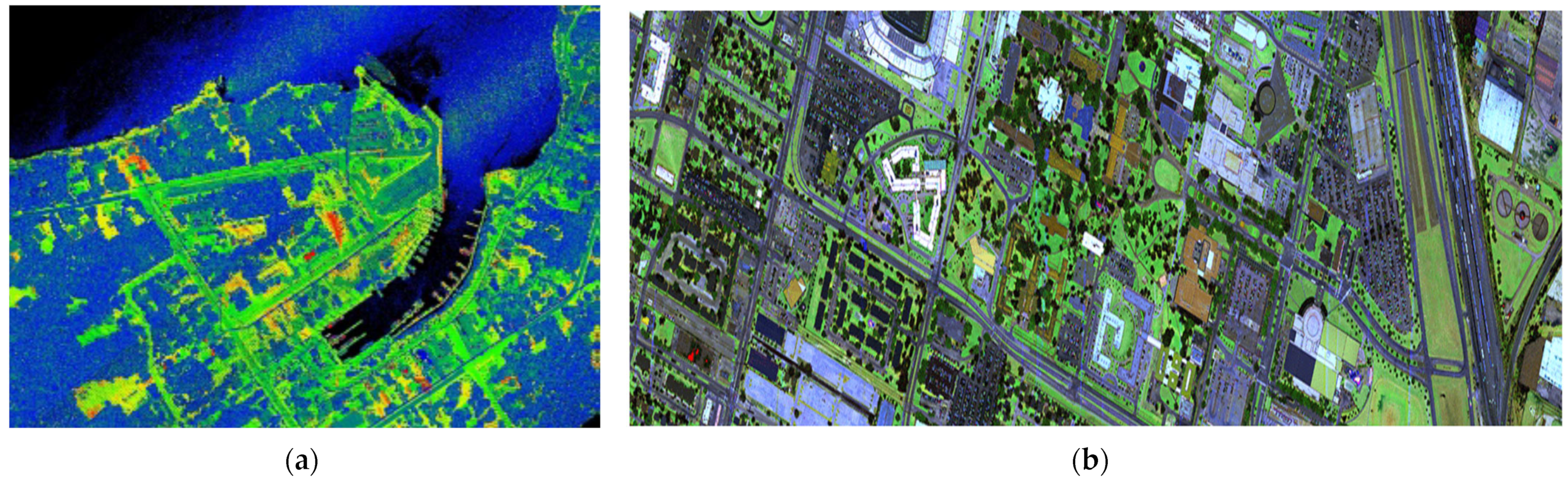
| ISPRS WG III/5, 2015 | ISPRS WG III/5 and Teledyne Optech | 3D | Optech Titan | SWIR, NIR, and green | Natural coastal | Tobermory (ON, Canada) | NA |
| IEEE GRSS, 2018 | NCALM | 2D | Optech Titan | SWIR, NIR, and green | Urban | University of Houston campus and its neighborhood | RGB and hyperspectral image |
| Application | Potentials | Opportunities | Challenges |
|---|---|---|---|
| Ecology and forestry | Gathering spatial-spectral information from canopies and under canopies Vegetation indices | Aiding plant/tree species classification Increasing accuracy of individual tree segmentation and wood–leaf separation Physiological and health condition analyses More accurate estimation of other tree parameters | Better exploit plant reflectance in the different wavelengths Improve characterization of single species |
| Objects and LULC classification | Incorporating spectral features Built-up indices | Fine-grained 3D uraban mapping Facilitating detecting ground-level objects Proposing single-data source solution | Understand relationships between wavelengths and needed classes A proper radiometric calibration is necessary to reduce systematic differences between radiometric strips |
| Change detection | More precise automated monitoring of surface changes | Replace visual interpretation of multi-temporal images | Upscaling, costs, appropriate radiometric calibration |
| Bathymetry | Richer spectral information Water indices | More accurate water surface mapping Monitoring of hydromorphological status | Dealing with other challenging shore areas (e.g., delta wetland, rocky shore, and shore with land depression) |
| Topographic mapping | Improved DTM generation by using spectral information | Detailed DTM/DSM separation | Filtering areas with water |
| Archaeology and geology | Different reflectance behavior of object at different wavelengths | Preserve historical buildings Detecting the damaged areas of building Geological material detection and classification Supporting mining operations Tunnel modeling Mineral disaster prevention | Appropriate wavelength selection with respect to the actual surface status Systematic radiometric strip differences should be reduced by a proper radiometric calibration process |
| Navigation | Requiring less illumination power Less prone to motion blur Providing useful information of material-specific spectral signatures | Autonomous driving Assisting point cloud matching in SLAM Higher scene recognition accuracy in a complicated road environment | Detection of multiple hundreds of photons per wavelength channel is required for achieving high accuracy Optimal channel selection should be carried out |
Disclaimer/Publisher’s Note: The statements, opinions and data contained in all publications are solely those of the individual author(s) and contributor(s) and not of MDPI and/or the editor(s). MDPI and/or the editor(s) disclaim responsibility for any injury to people or property resulting from any ideas, methods, instructions or products referred to in the content. |
© 2024 by the authors. Licensee MDPI, Basel, Switzerland. This article is an open access article distributed under the terms and conditions of the Creative Commons Attribution (CC BY) license (https://creativecommons.org/licenses/by/4.0/).
Share and Cite
Takhtkeshha, N.; Mandlburger, G.; Remondino, F.; Hyyppä, J. Multispectral Light Detection and Ranging Technology and Applications: A Review. Sensors 2024, 24, 1669. https://doi.org/10.3390/s24051669
Takhtkeshha N, Mandlburger G, Remondino F, Hyyppä J. Multispectral Light Detection and Ranging Technology and Applications: A Review. Sensors. 2024; 24(5):1669. https://doi.org/10.3390/s24051669
Chicago/Turabian StyleTakhtkeshha, Narges, Gottfried Mandlburger, Fabio Remondino, and Juha Hyyppä. 2024. "Multispectral Light Detection and Ranging Technology and Applications: A Review" Sensors 24, no. 5: 1669. https://doi.org/10.3390/s24051669
APA StyleTakhtkeshha, N., Mandlburger, G., Remondino, F., & Hyyppä, J. (2024). Multispectral Light Detection and Ranging Technology and Applications: A Review. Sensors, 24(5), 1669. https://doi.org/10.3390/s24051669