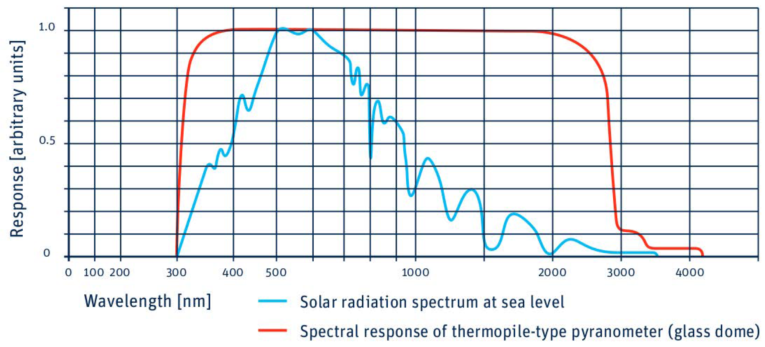
In this section, the case study with which the MAPSol model has been validated is precisely described, including the description and reliability of the chosen irradiance data and the generation of the high-resolution DEM of the study area, as well as the adapted grid, and the simulation with the MAPSol model. The chosen case study provides the possibility to assess the effect of shadows caused by the intricate orography generated by buildings close to the location of pyranometers.
3.1. Experimental Data Acquisition
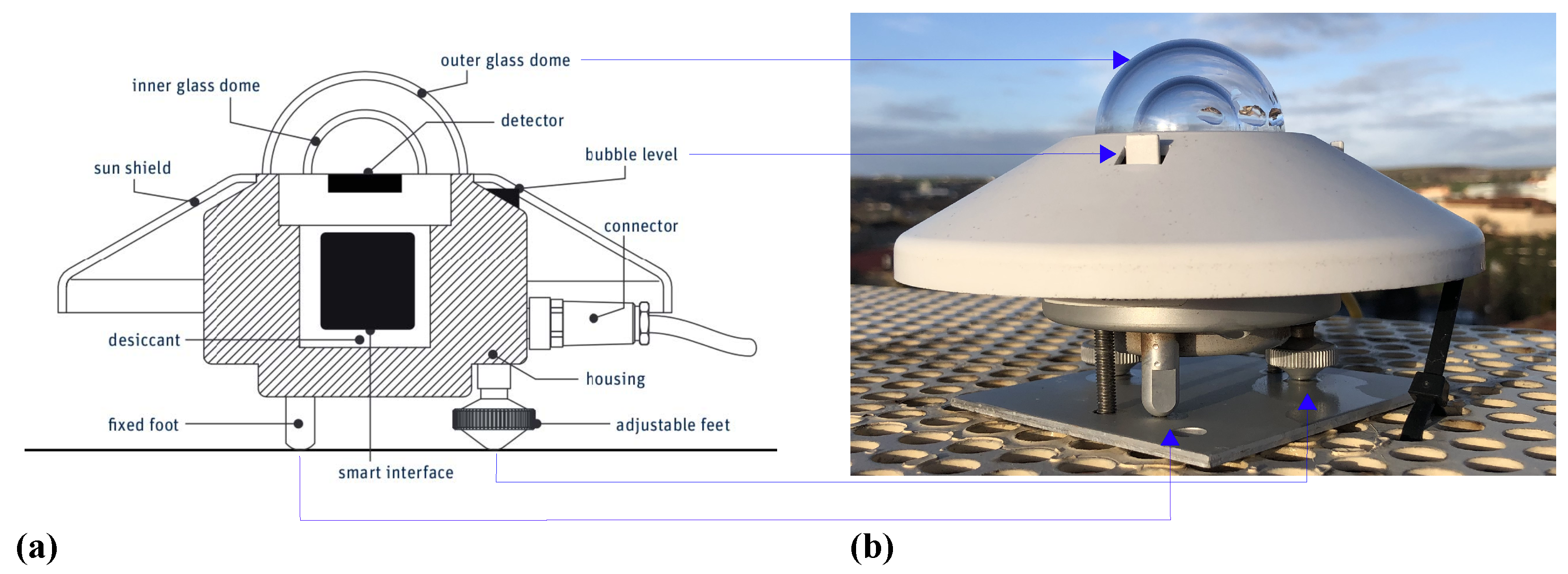
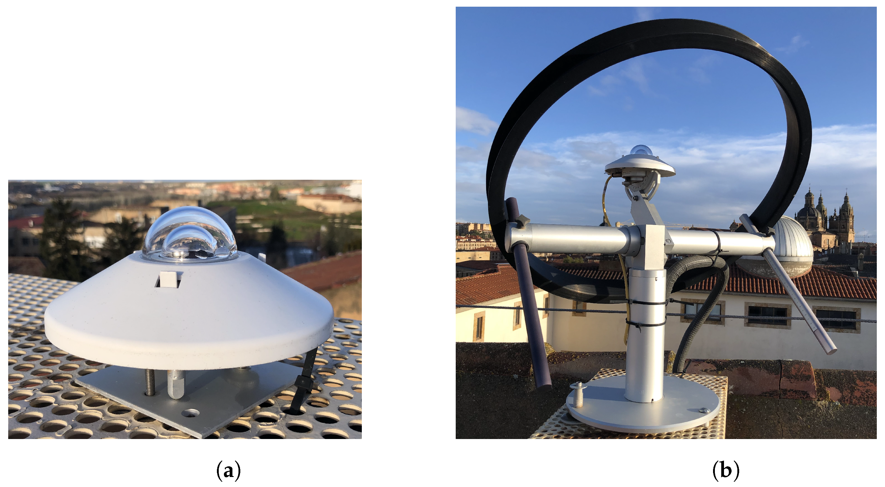
Experimental data were obtained from two pyranometers and a weather station, shown in
Figure 7, installed on the rooftop of the
Trilingüe building at the Faculty of Sciences (40.96062° N, 5.67075° W) of the University of Salamanca (Spain): a pyranometer Kipp and Zonen SMP10 (
Figure 7a) and a pyranometer SMP10 with shadow ring model Kipp and Zonen CM 121 (
Figure 7b).
During the day, the devices perform the corresponding measurements, storing and values every five minutes. At the end of the day, the collected data are sent to the computer, generating a csv file containing the irradiance information. The next step is to classify and filter the files. To do this, a program developed in “Mathematica® Software v. 13.1, Licensed to Universidad de Salamanca”, identifies the files that belong to the same day and extracts the desired information from each of them. Finally, the program generates a new output file where all the information for the same day is merged.
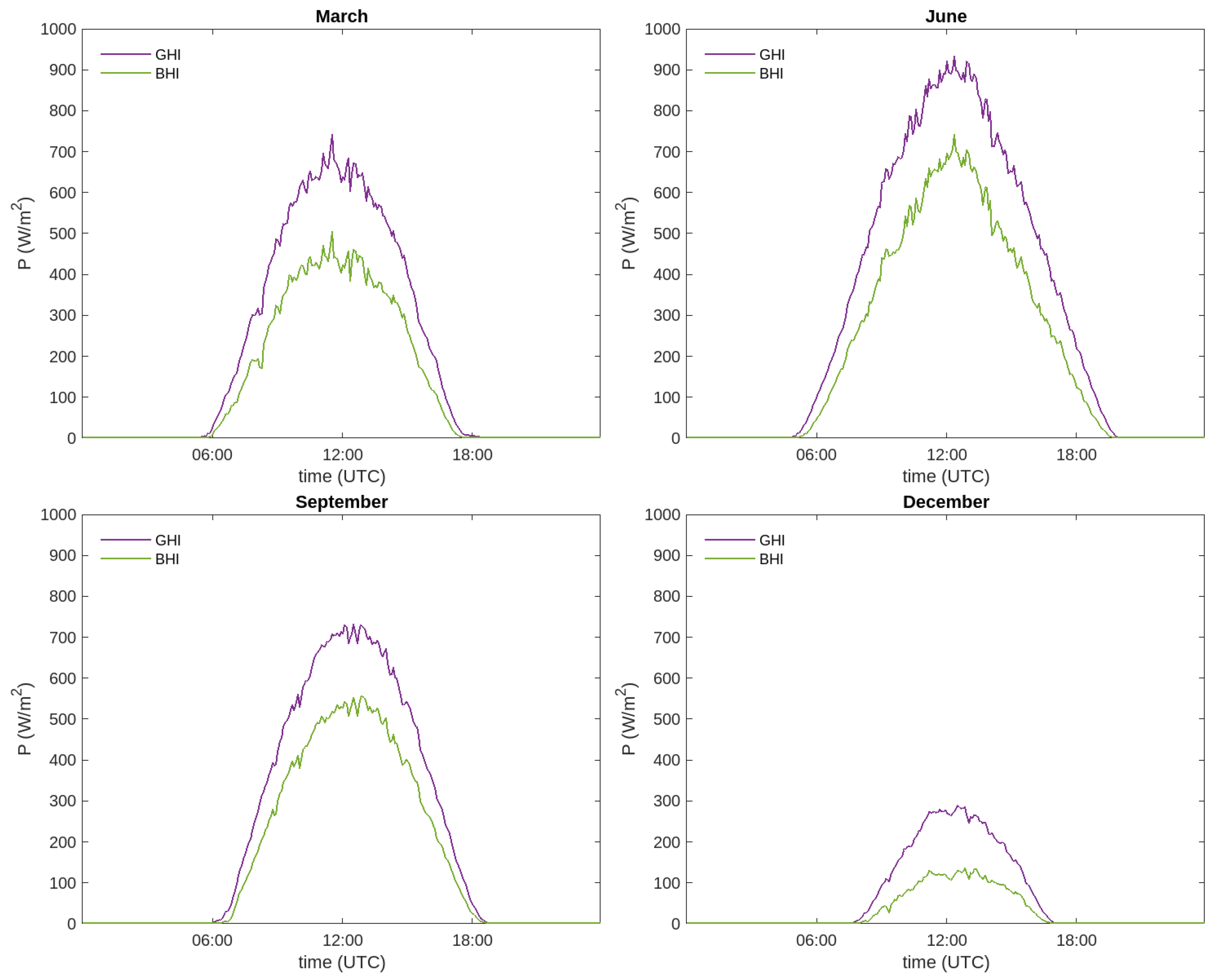
The results presented in this work have been obtained with data between 30 July 2020 and 22 February 2023. In
Figure 8, illustrative monthly averages have been performed on the irradiance, so that for each month,
and
curves are obtained as a function of time (which is represented in the UTC format). The monthly average is obtained by considering the data of all the days belonging to that month in the whole study period.
As previously mentioned, pyranometers take measurements of
and
. To obtain the
component, a correction factor which depends on the day of the year is required. For each of the measurements, the correction factor is calculated as a function of the solar declination angle, and hereafter,
is considered to include the correction factor. The
and
measurements are obtained, every 5 min, from Equations (
1) and (
2), respectively. During the night,
and
values should be identically zero, but it is found that negative values appear. This is usual when performing this type of measurements. However, it does not make physical sense to work with negative irradiances. To solve this problem, the following filters are introduced into the program:
If
If
If
If
The irradiance curves introduced below are intended to be as close as possible to the actual measurements, so no statistical treatment beyond averaging is carried out.
Figure 8 shows the irradiance curves for four representative months of the year: March, June, September and December. In all these plots, a certain level of noise is observed within the irradiances, which evinces that the pyranometers are very sensitive to small changes. For example, on a summer day with isolated clouds, if a cloud comes between the Sun and the pyranometer for a few minutes, the direct components will become very small. When the cloud has passed, the direct component will again reach high values. When observing the set of figures, it can be noticed that the irradiance curves increase in width and height in the summer months. On the contrary, during winter, when the Sun is up for less time and at a lower height above the horizon, the curves become narrower and present lower peak values.
In order to assess the reliability of the measurements obtained, these values are compared with two independent external sources: AEMET [
51] and Solargis [
52] for solar irradiance. The Atlas of Solar Radiation in Spain, using data from the EUMETSAT climate FAS developed by AEMET [
51], uses satellite data with a spatial resolution of
km. Data from the period (1983–2005) were used to elaborate the atlas. In order to compare the results in a more convenient way,
Table 3 shows the results of this work compared with those of AEMET. The relative differences obtained for 9 of the 12 months of the year do not overcome 10% in the daily accumulated energy for the global component (
). This number is reduced to eight for the direct horizontal component (
).
Taking the experimental data of
and
from
Table 3, it is possible to obtain the annual cumulative values and also the average value per day of the energy received. The annual cumulative values are easily obtained by performing the following operation:
where
x represents the irradiance component, the subscript
i is the number of the month, and
is the number of days in month
i.
The Atlas of Solar Radiation in Spain [
51] using data from the EUMETSAT climate FAS provides daily average
and
values in the form of an irradiance distribution map. The values extracted from these maps can be seen in
Table 4, together with the values recorded in situ.
The value for obtained in this work is within the AEMET interval, touching the upper limit. The experimental component is 0.01 kWh above the maximum value of the interval. AEMET does not offer the annual average accumulated values, but they can be calculated by multiplying the daily average by the number of days in the year (the result is also shown in the same table). Again, the experimental value of is within the range, while the value of is slightly above it.
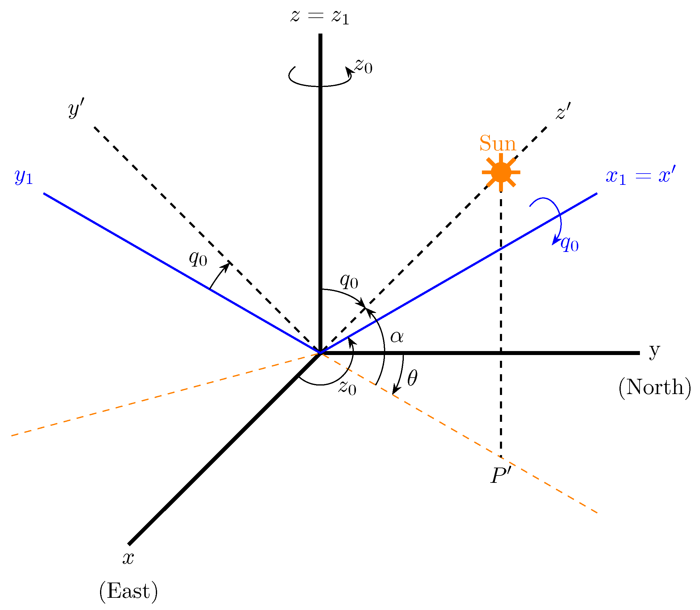
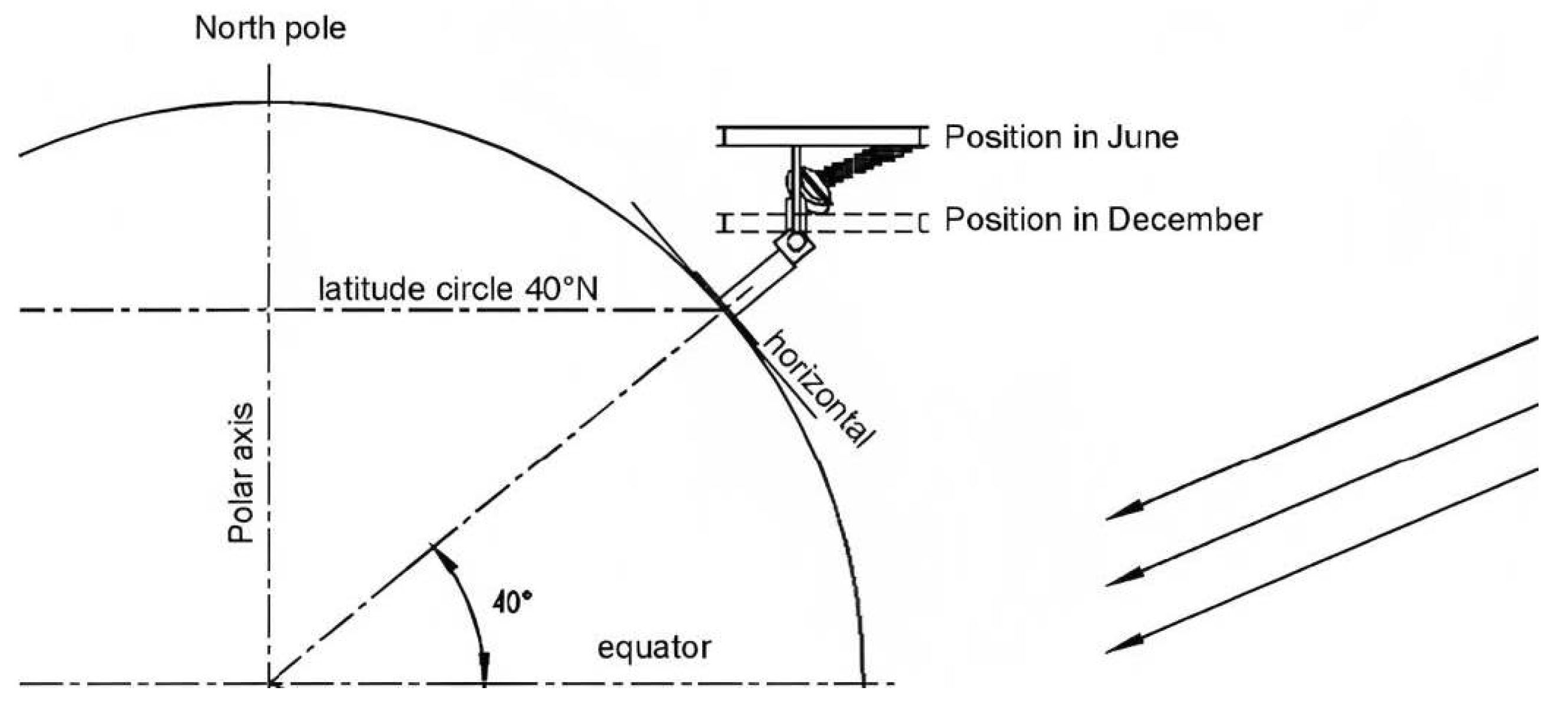
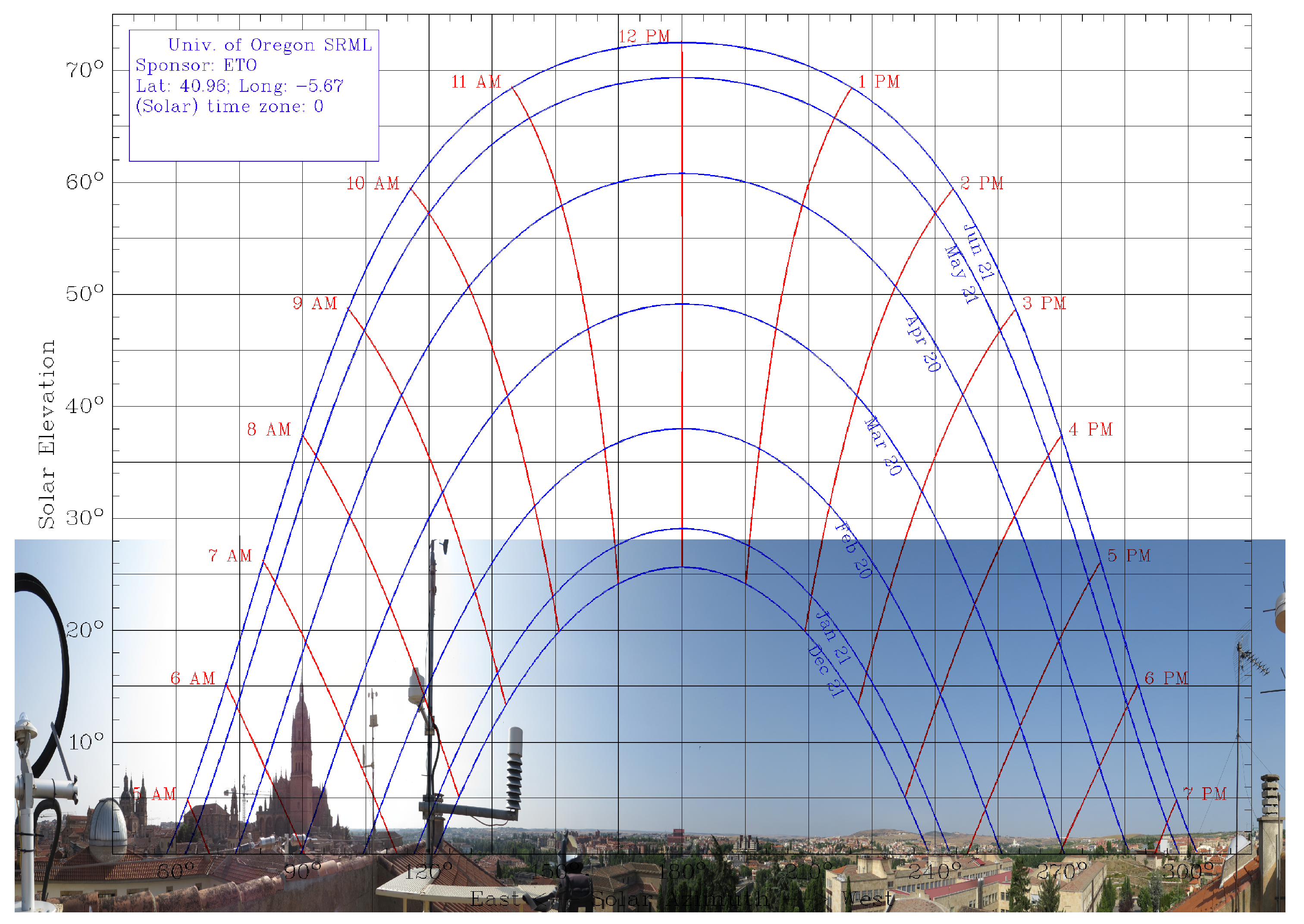
As it is known, a Sun chart is employed to present, at a specific location, the apparent position of the Sun, i.e., the height of the Sun at any hour of the day. From a Sun chart elaborated by the University of Oregon Program [
53], together with a panoramic photo from the
Trilingüe building at the University of Salamanca,
Figure 9 is elaborated. This figure shows the Sun path chart from the
Trilingüe building at the University of Salamanca (40.96062° N, 5.670759° W) between 21 December and 21 June, overlapped with a panoramic photo, taken from a pyranometer that registers
to identify shadowing sources.
One of these shadowing sources on the location of the pyranometers is the 93-m-high cathedral tower, located 296 m to the east. As can be seen in
Figure 9, the cathedral tower casts its shadow in this area during the early hours of some days of the year, specifically between 22 August and 11 September, and in its symmetrical months, February and March. In these months close to spring, cloudiness is higher, so it is more difficult to obtain irradiance measurements that allow the effect of the cathedral’s shadow to be clearly seen. However, in summer, the sky is clearer, and this phenomenon can be seen more clearly in the measurements obtained.
3.2. Area Study, High-Resolution DEM and Adapted Mesh
An area of 430 m × 176 m has been selected which includes the Trilingüe building at the Faculty of Sciences of the University of Salamanca, where the pyranometers are located, and the cathedral tower located at 296 m in a straight line to the east, which casts its shadow on the pyranometers affecting the reading of the irradiance data.
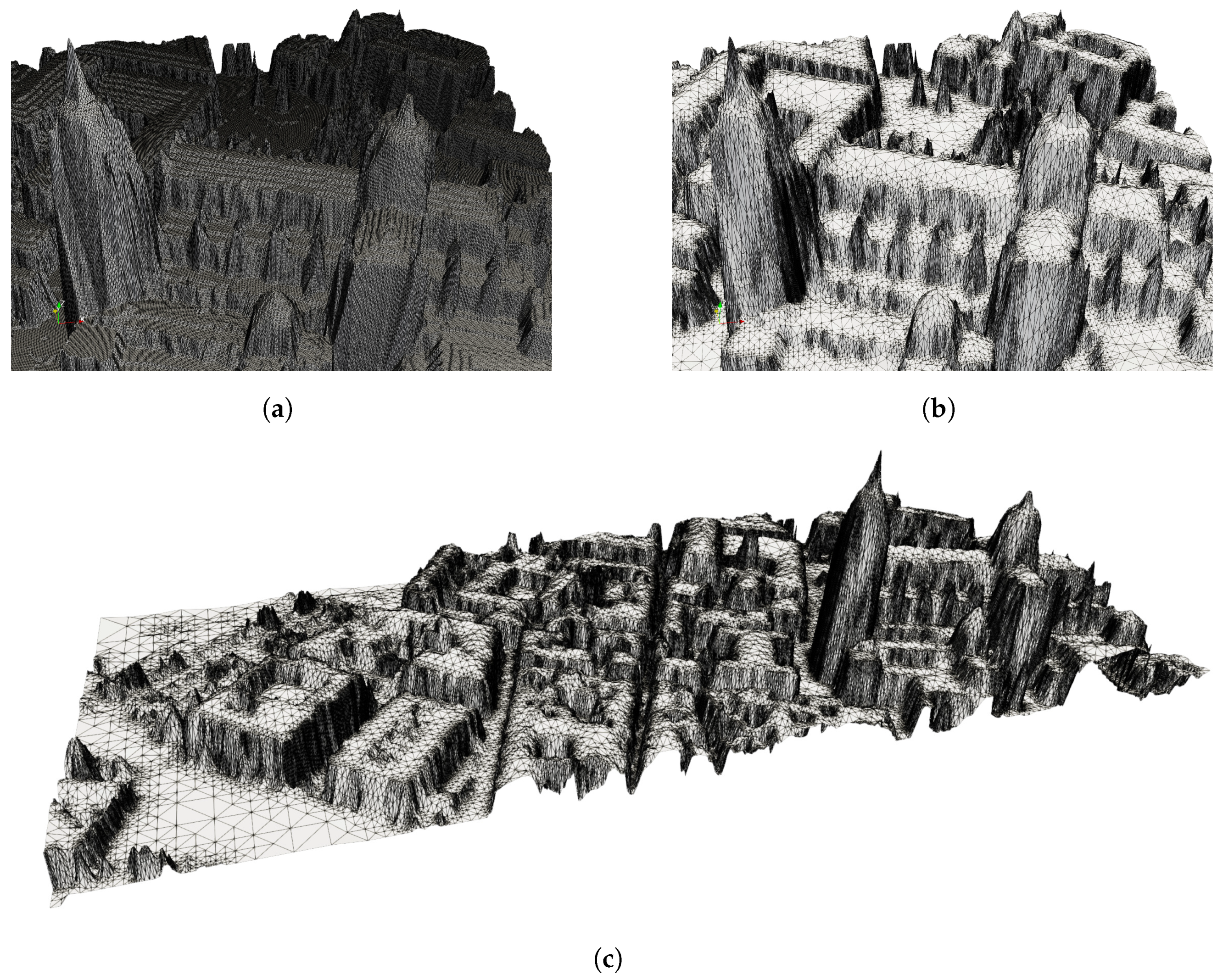
Provided with the point cloud available in the area under study, the DEM generated with the process described in
Section 2.3 presents a resolution of 33 cm (
Figure 10). This methodology performs the generation of the Delaunay triangulation using negligible computing time (3 s for
points and
triangles), with a computer with Intel Core i7-6700 processor at 3.41 GHz, 64 bits, 32 Gb. RAM and 931 Gb (Dell Precision Tower 3620, Round Rock, TX, USA).
The size of the raster file is too large for the calculations involved in the MAPSol model, so the mesh is adapted using the procedure described in
Section 2.4, achieving a reduction of
in the number of cells. The adapted mesh for a tolerance of 1 m has
triangles and includes all the singularities of the study area, in particular the cathedral tower. This element holds significant importance in the DEM. It is not present in some of the raster files, such as those provided by the IGN (Digital Surface Model–Building and Digital Surface Model), due to their low resolution and dimensions.
The number of triangles can be further reduced without affecting the accuracy of the shadow and irradiance calculations, using a tolerance of 5 m. This means that in the mesh adaptation process, a triangle is refined if the distance from the triangle to the high-resolution DEM is greater than 5 m, or 1 m in the previous case. The number of triangles of the adapted mesh with a tolerance of 5 m is , which represents a reduction of more than with respect to the original mesh, without, as we will show further, a significant loss in precision in the calculation of shadows and irradiance, but with a considerably lower computational cost.
Figure 11c displays the fine adapted mesh (1 m) for the entire study area and several zooms of both meshes, the fine adapted mesh (
Figure 11b) and the uniform original mesh (
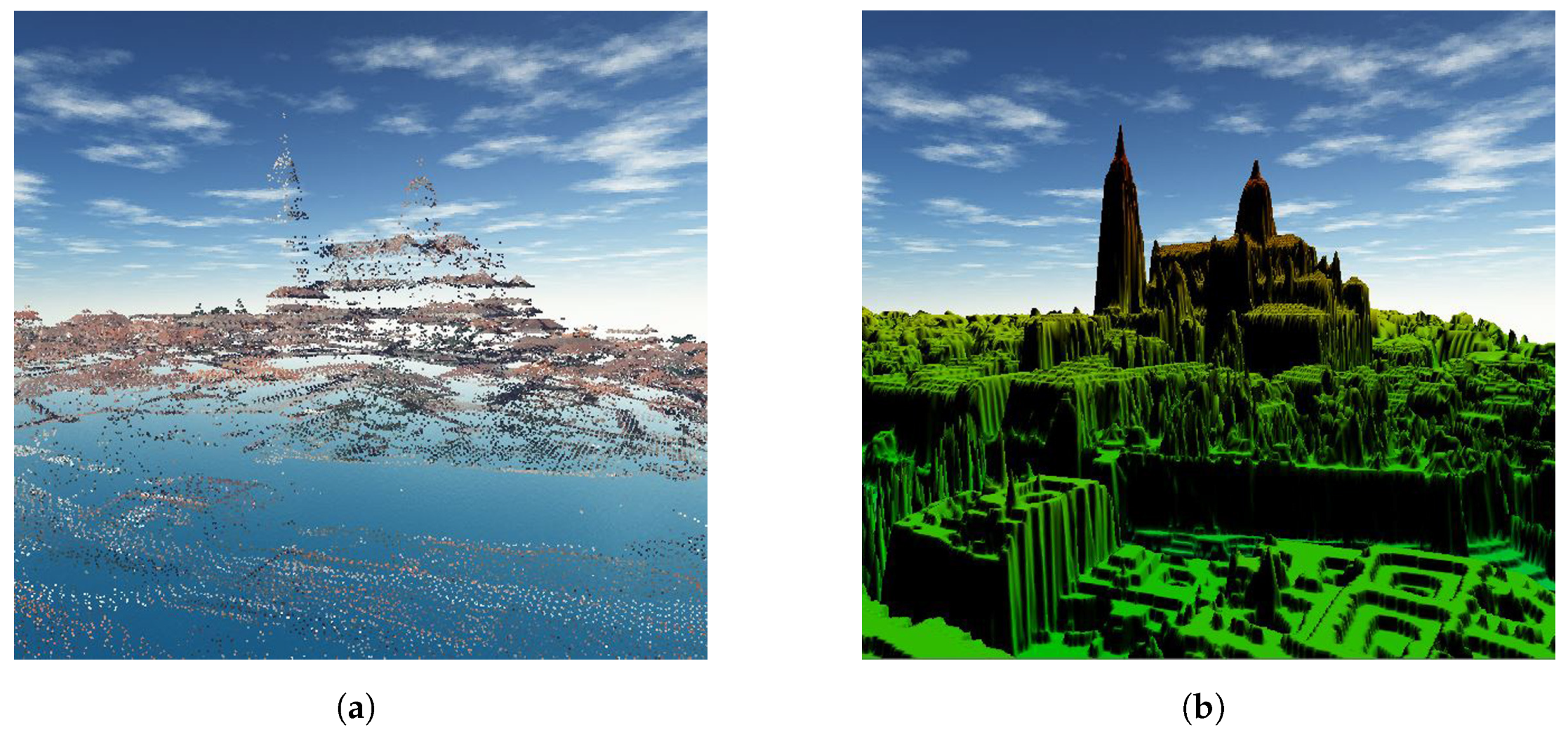
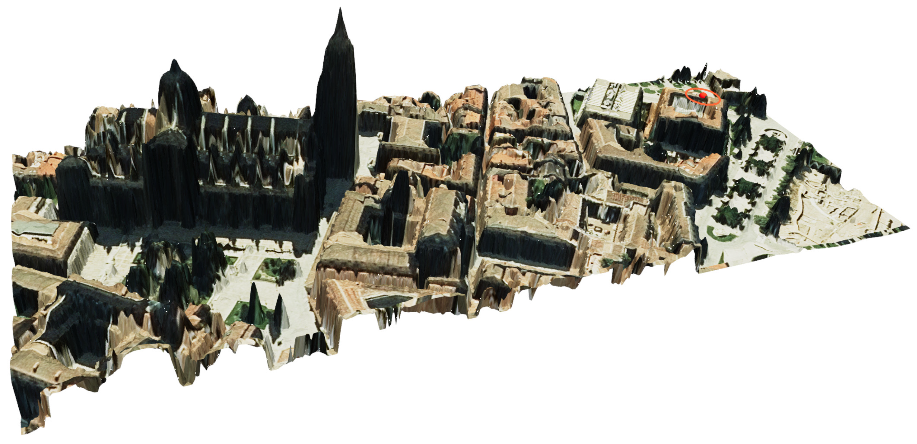
Figure 11a), for the Cathedral building area. A 3D reconstruction of the study area is depicted in
Figure 12, including the location of the pyranometers with a red point, which allows the complexity of the study area to be observed. Furthermore, this procedure demonstrates that with few free resources, it is possible to reconstruct a 3D image of a very complex area such as this one, in the old part of the city of Salamanca. For
Figure 12, the most appropriate orientation has been chosen so that the orthophoto of the area projected on the fine adapted mesh provides the best visual result.
3.3. Simulation with MAPSol
Using the coarse adapted mesh (5 m), the shadows and global irradiance in each triangle have been calculated for each day for a full year, with a time step of 5 min, with the MAPSol model. Computations have been performed in a computer equipped with two AMD EPYC 7313 CPUs, 128 GB of RAM memory and Debian Linux version 11 operating system. MAPSol is written in Python and C++, using the latter for the core of the computation and the former mostly to deal with input/output. In this particular work, Python 3.9.16 version and GNU g++ 10.2.1 C++ compiler have been used. Simulations have been performed in parallel, using one core per month. The mean wall clock execution time was 3 h and 56 min, including writing results to files for later analysis.
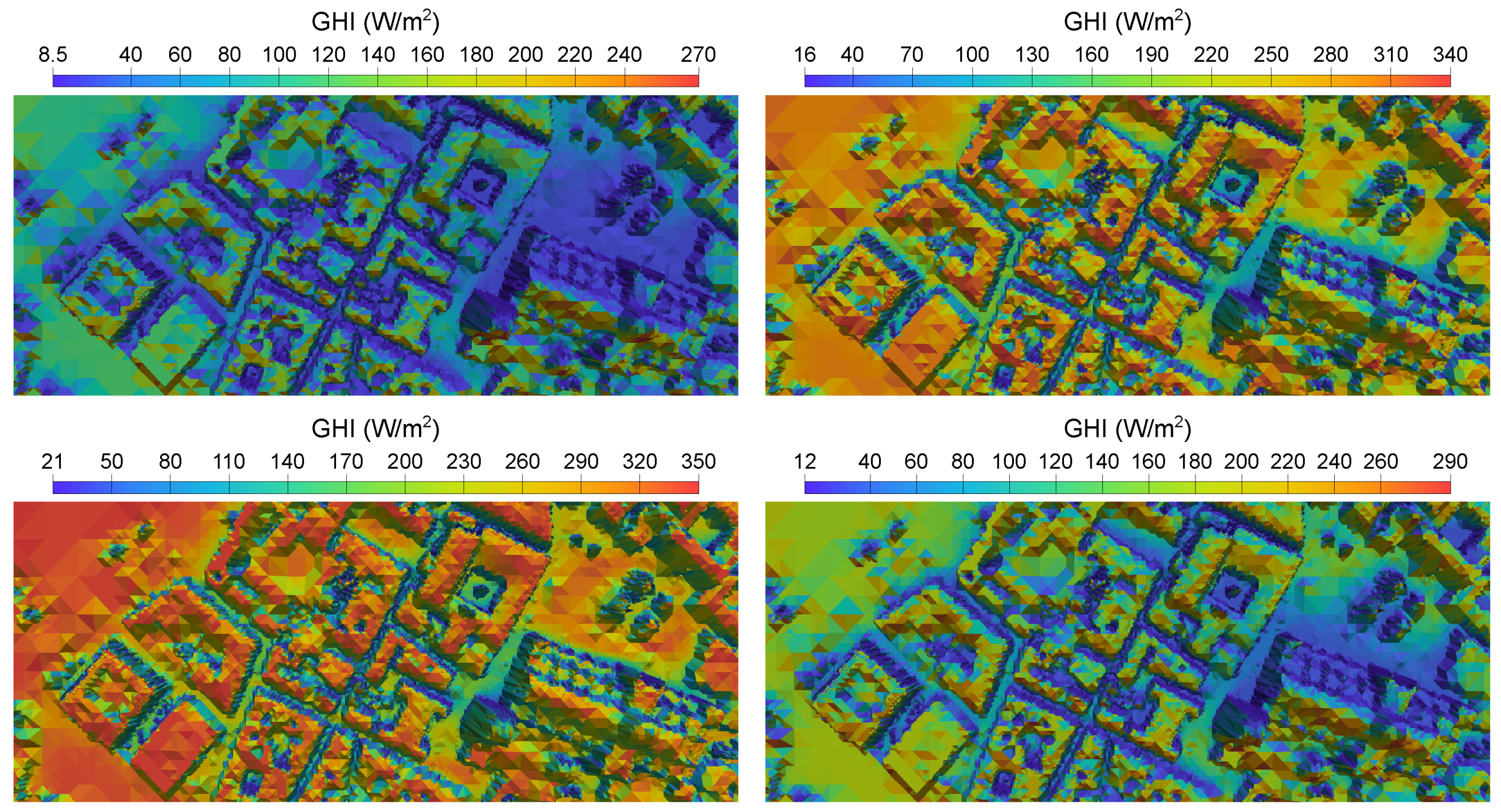
For each time step, a VTK file representing irradiance in the whole domain is written, as well as a csv file with values of GHI in the location of the pyranometers. Monthly average values of global irradiance in the study area have been calculated, and in
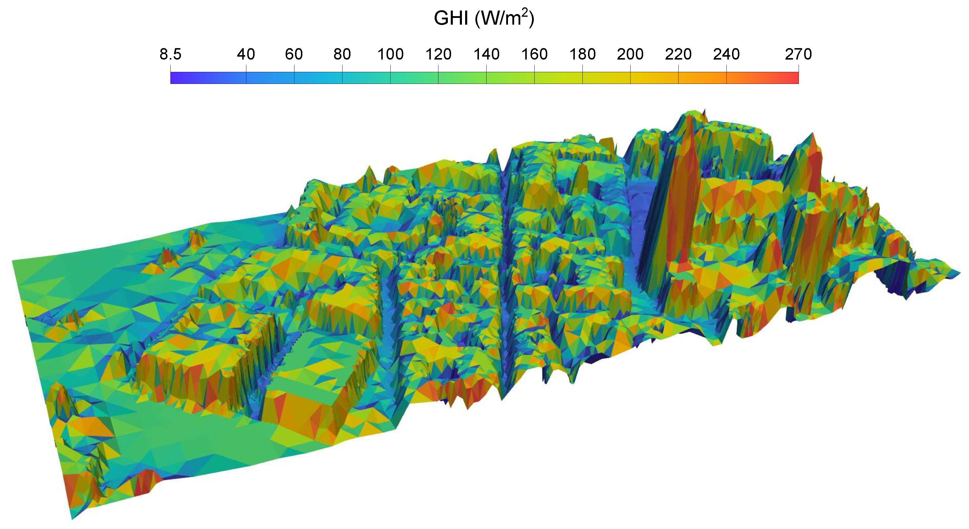
Figure 13, four of the most significant months of the different seasons of the year have been represented. In addition, the annual mean GHI is depicted in a 3D image in
Figure 14; notice that a view from the south has been chosen so that the facades most exposed to solar radiation can be appreciated.
Optionally, additional VTK files representing shadows cast in the domain for each time step can be obtained.
Figure 15 represents the computed shadows cast in the study area on 4 September 2022 at 7.00 a.m., when the shadow of the cathedral tower, located in the blue dotted square, affects the reading of the pyranometers, located in the red dot.
3.4. Comparison of Simulation Results with Experimental Data
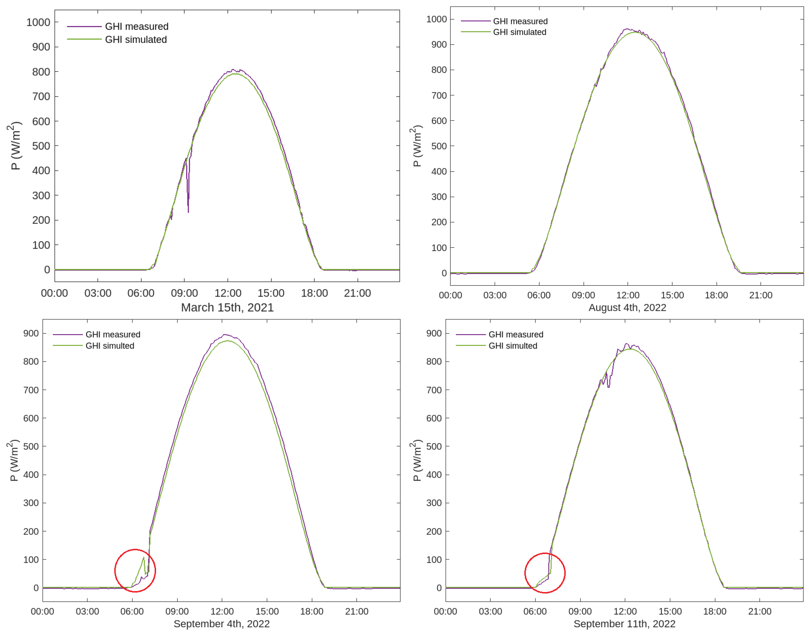
Taking into account the availability of data, due to cloud cover, possible technical difficulties and the reduced number of days on which the effect of the cathedral tower on the location of the pyranometers can be seen, the following dates have been chosen to compare the measured and calculated : 4 and 11 September 2022, when the measurements will show the effect of the shadow of the cathedral, and 15 March 2021 and 4 August 2022, when the shadow phenomenon will not occur.
Both measured and calculated
values have been taken every 5 min throughout the 24 h of the day, with a total of 288 data points. In the two lower graphics of
Figure 16, it can be clearly appreciated that the model captures the effect of the shadow of the cathedral in the early morning. The cathedral tower shadows the pyranometers just at sunrise, causing an interruption in the increase in irradiance, either with a sharp and short decrease (
Figure 16, bottom left) or with a sharp and delayed sunrise (
Figure 16, bottom right). Both phenomenologies are well captured in the simulation, with the pyranometer measurement (purple line) matching the calculated
(green line) very accurately. The upper graphics correspond to two dates where the shadow of the cathedral does not affect the irradiance data reading. The upper left graph shows the effect of cloud cover around 9 a.m. on pyranometer measurements (purple line).
To compare the accuracy of the results and the computational cost, the selected days were also simulated using the high resolution (1 m) mesh. The results at the pyranometer’s locations are the same (with 6-digit accuracy) as those obtained using the 5 m mesh, but the mean execution time is 68 times higher, so the 5 m mesh was chosen for all irradiance simulations. However, the use of the high resolution mesh might be appropriate in case a very precise study of shadows over the whole domain is intended.
In order to evaluate the precision of the model for a clear sky, four representative statistical error indicators have been calculated for the selected dates.
: Mean Absolute Error
: Normalized Mean Absolute Error
: Root-Mean-Square Error
: Normalized Root-Mean-Square Error
: Coefficient of determination
Here,
and
represent, respectively, the measured and calculated value of the global irradiance at time
, corresponding to the
time instants for which data are available.
refers to the maximum measured
, and
is the mean of the measured GHI.
Table 5 summarizes the statistical indicators described above for the four selected days, showing very small values, especially the normalized errors, resulting in a higher coefficient of determination (
).


 ,
, 


