
Optimal Design of Sparse Matrix Phased Array Using Simulated Annealing for Volumetric Ultrasonic Imaging with Total Focusing Method

Abstract
:1. Introduction
2. Theory
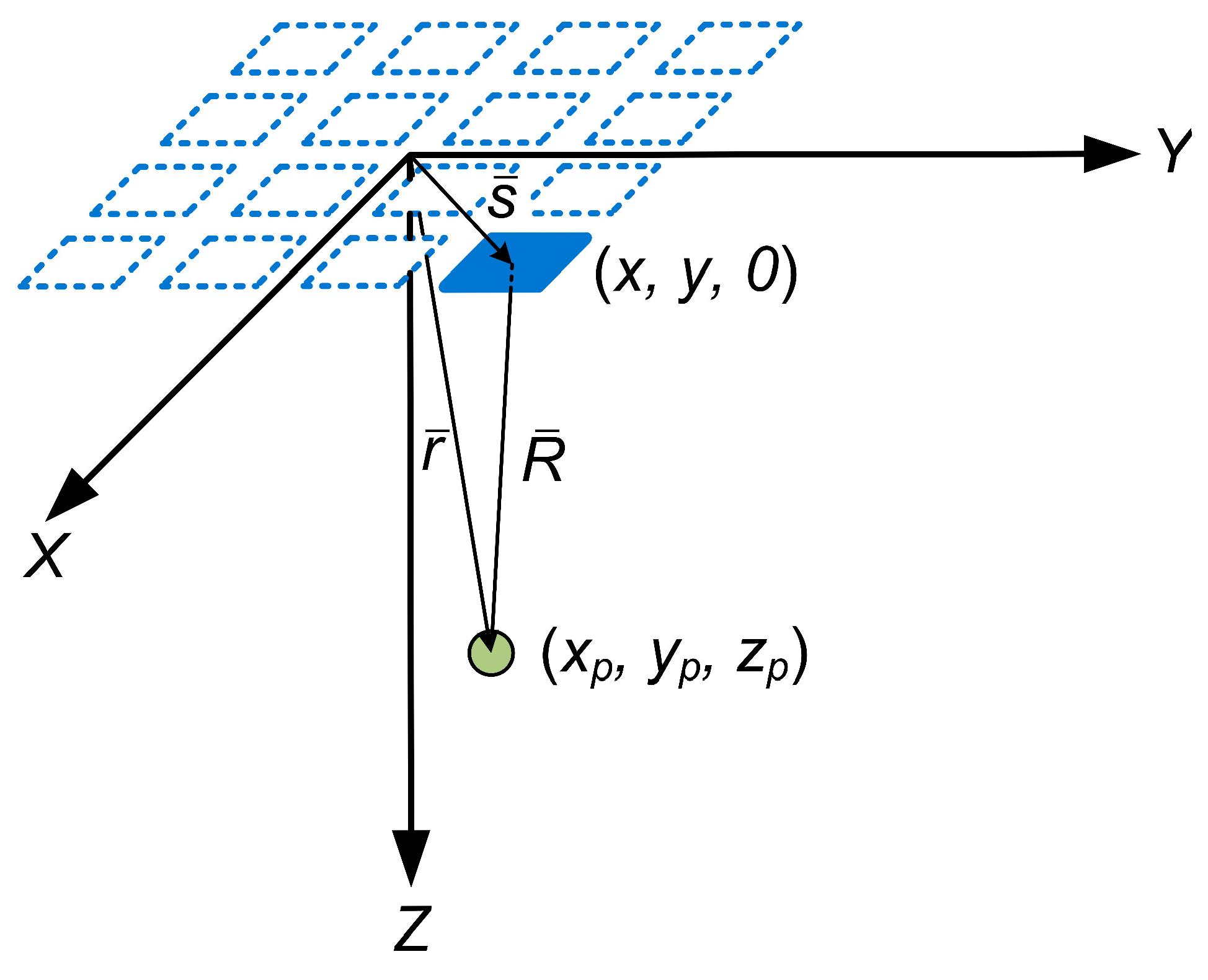
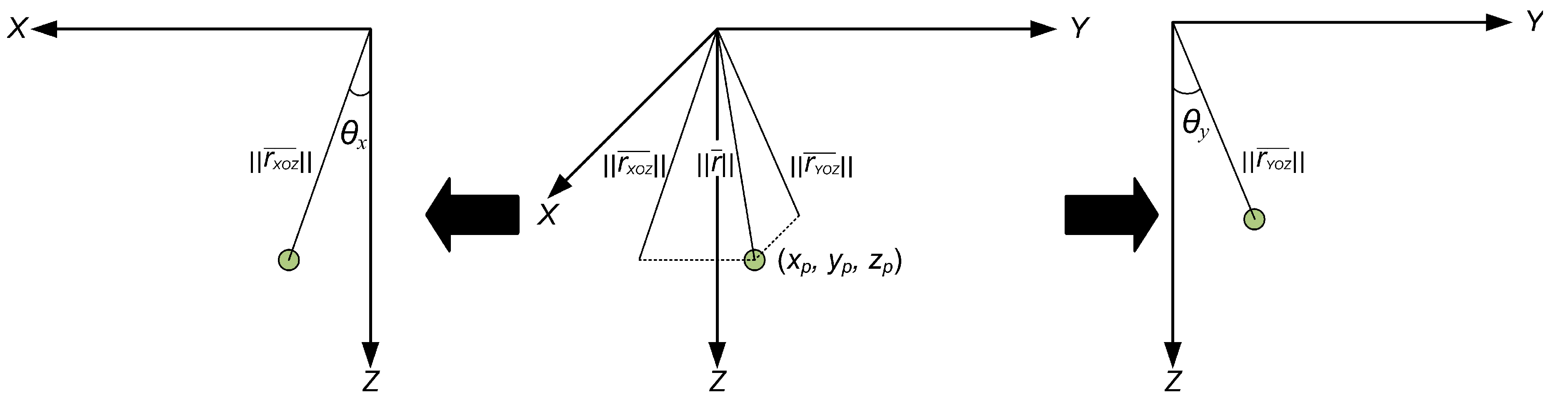
2.1. Beam Directivity Function of Matrix Phased Arrays
2.2. Simulated Annealing Algorithm
3. Determination of the Optimal Sparse Matrix Phased Array Configuration Using the Simulated Annealing Algorithm
3.1. Simulated Annealing Algorithm Implementation
- The number of elements in the matrix phased array;
- The center frequency of the probe elements;
- The pitch of the array and the dimensions of each element;
- The velocity of the ultrasonic waves in the test object;
- The number of active elements in the sparse matrix phased array configuration.
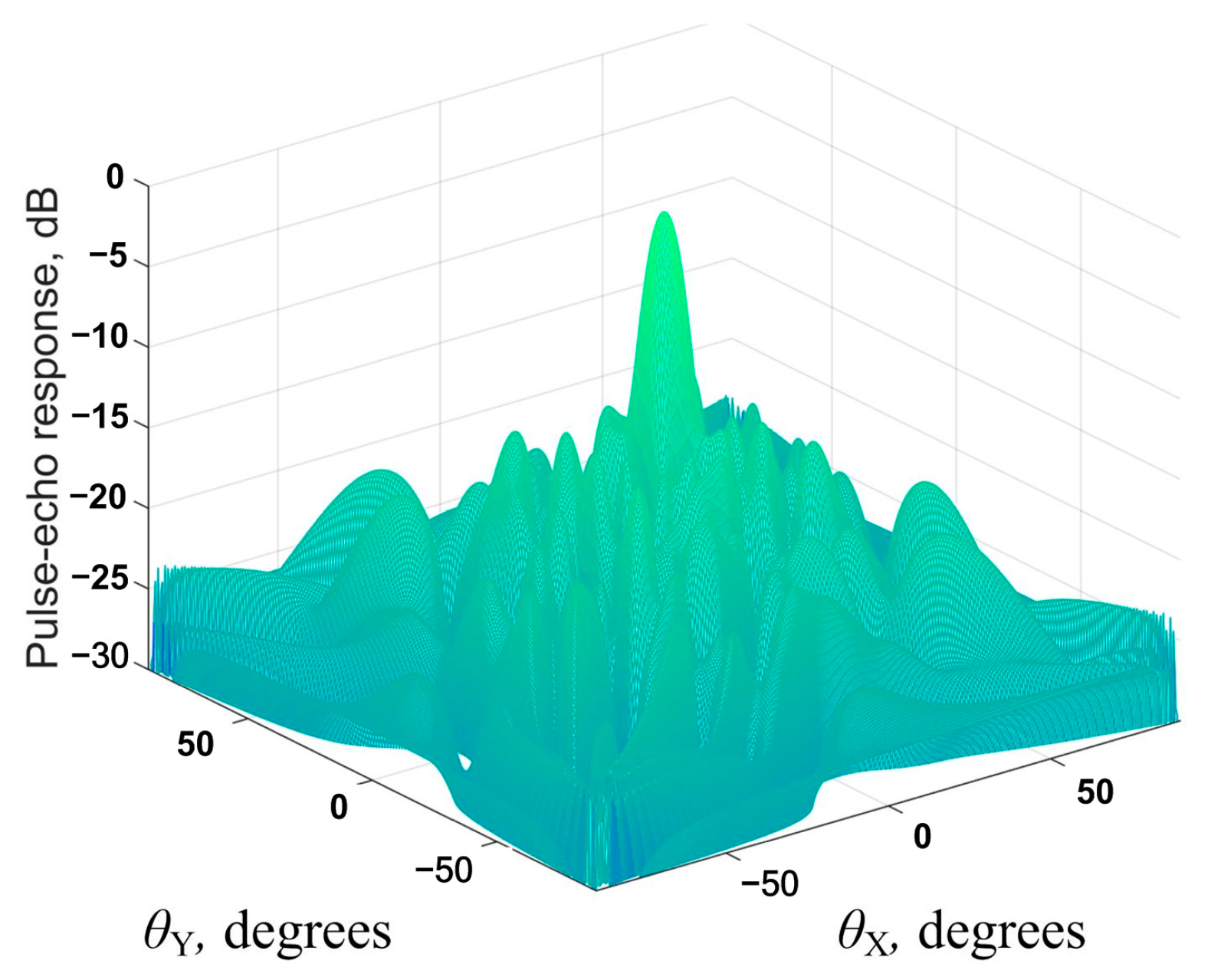
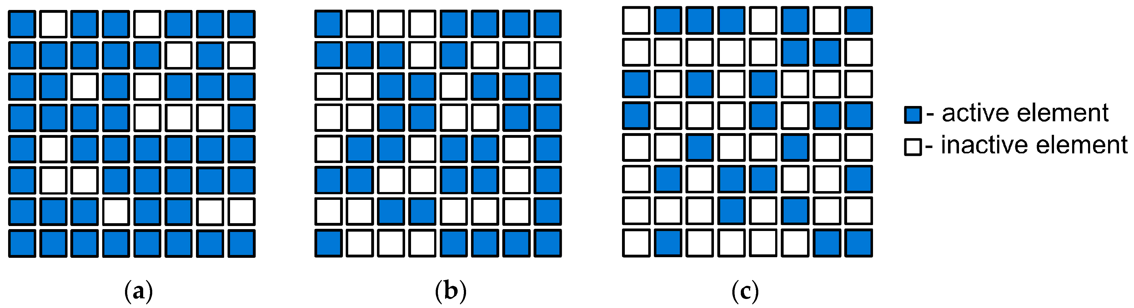
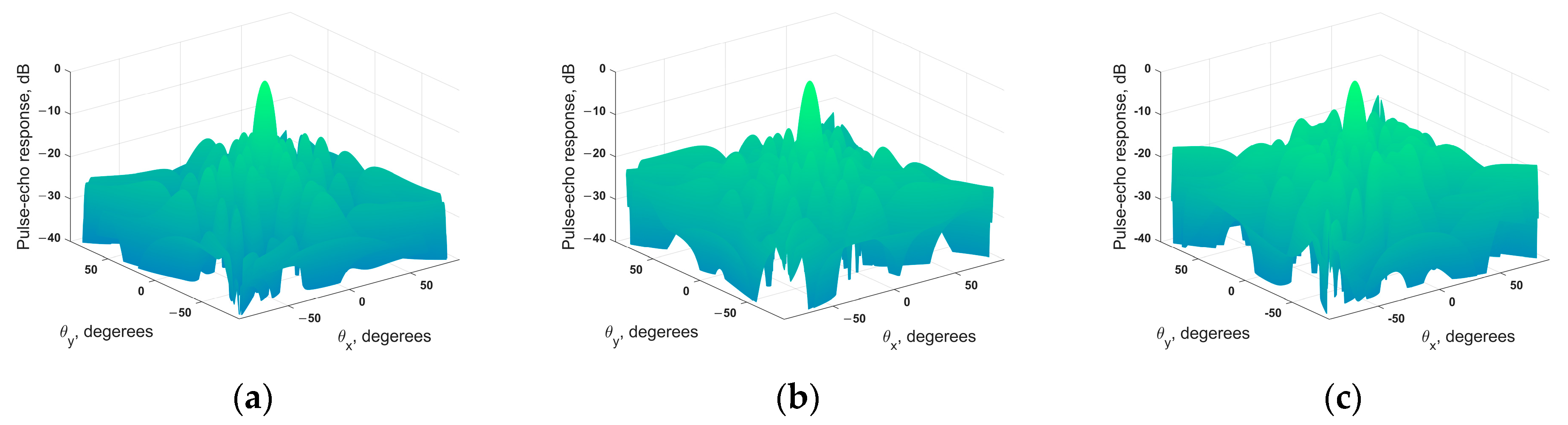
3.2. Results of Simulated Annealing Algorithm Execution
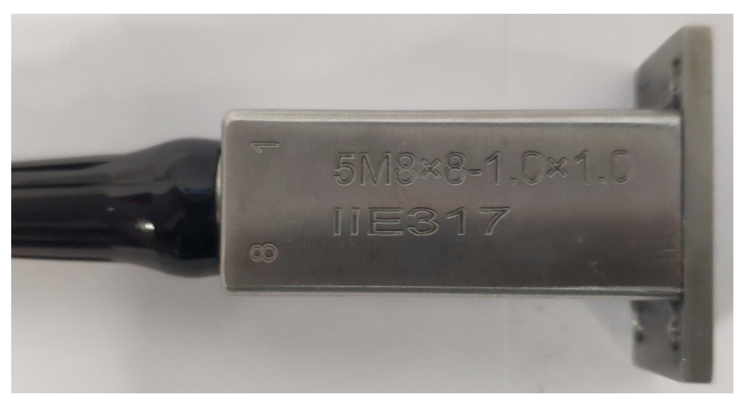
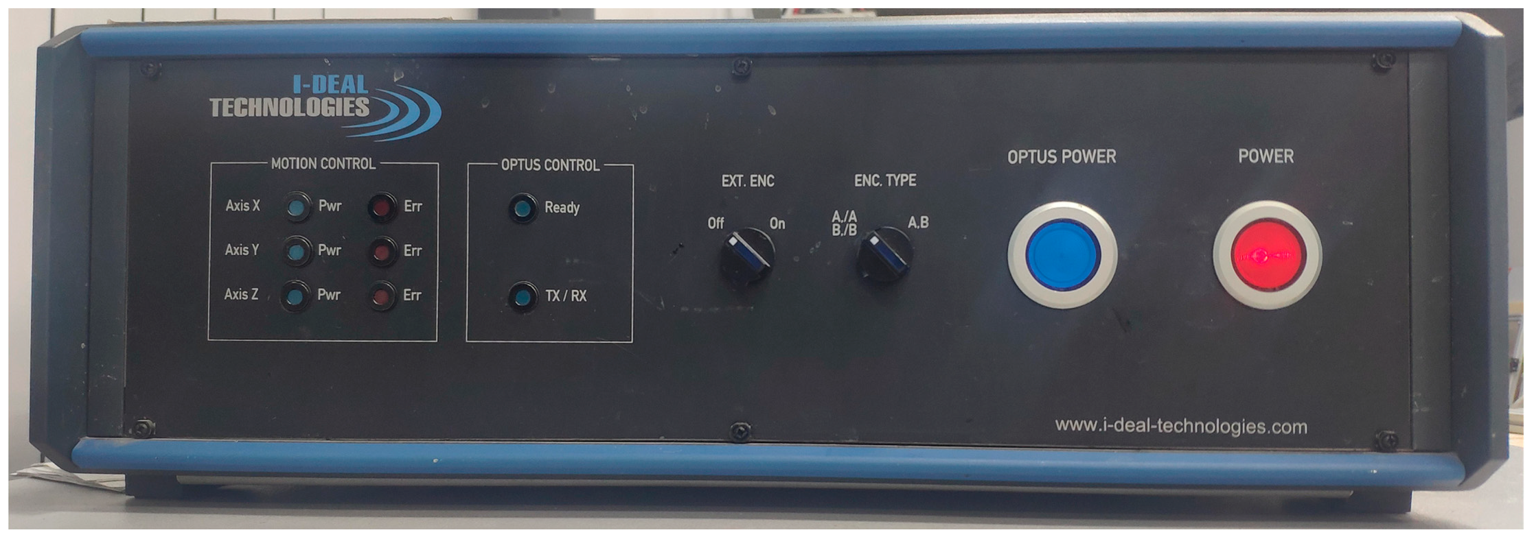
4. Experiments
- SNR is higher than 20 dB;
- the level of artifacts relative to the amplitude of the flaw in the image is less than 20 dB;
- the image of the entire flaw boundary is restored.
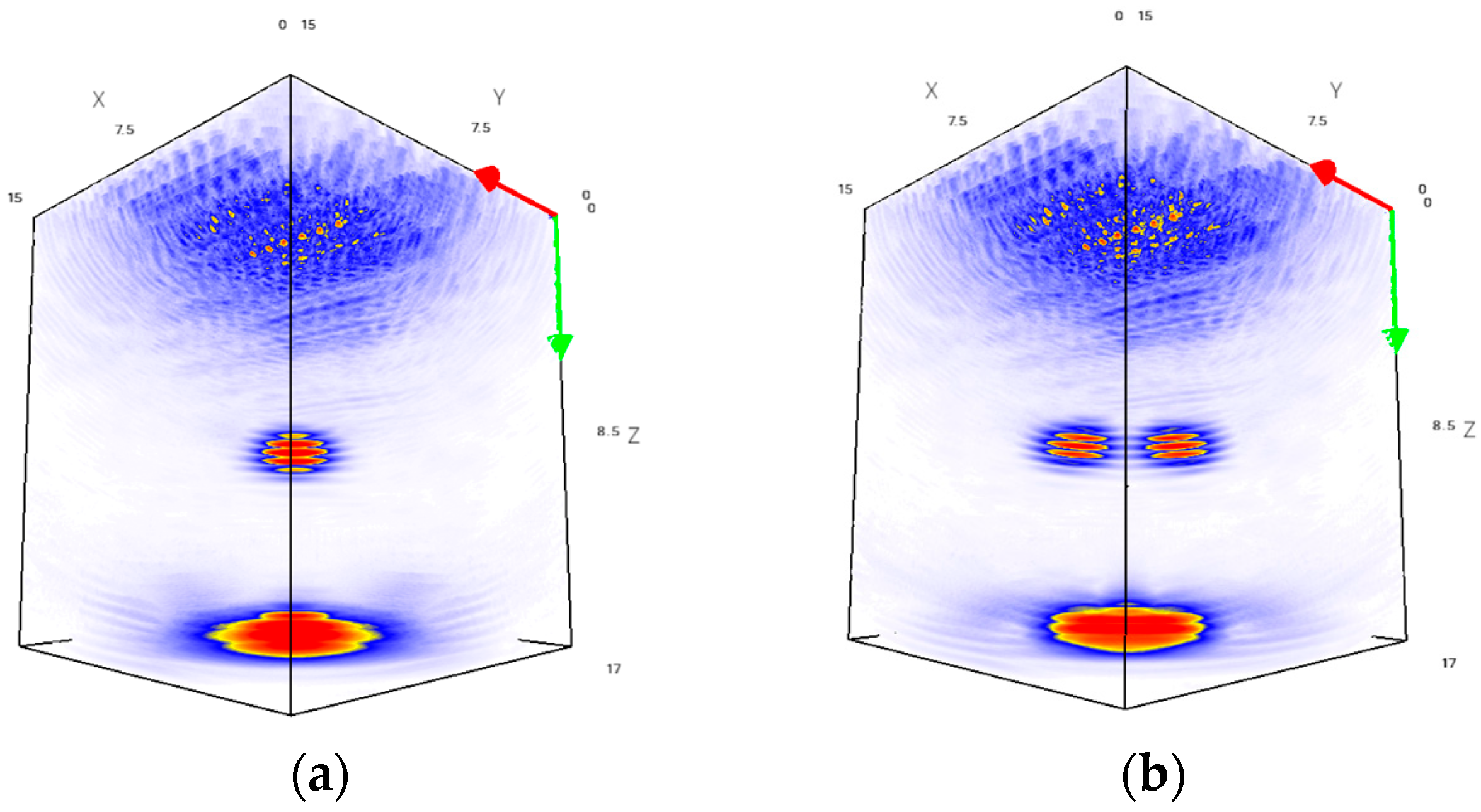
5. Results and Discussion
6. Conclusions
Author Contributions
Funding
Data Availability Statement
Acknowledgments
Conflicts of Interest
References
- Long, R.; Russell, J.; Cawley, P. Ultrasonic phased array inspection using full matrix capture. Insight 2012, 54, 380–385. [Google Scholar] [CrossRef]
- Holmes, C.; Drinkwater, B.W.; Wilcox, P.D. Post-processing of the full matrix of ultrasonic transmit–receive array data for non-destructive evaluation. NDT E Int. 2005, 38, 701–711. [Google Scholar] [CrossRef]
- Cruza, J.F.; Camacho, J. Total Focusing Method with virtual sources in the presence of unknown geometry interfaces. IEEE Trans. Ultrason. Ferroelectr. Freq. Control 2016, 63, 1581–1592. [Google Scholar] [CrossRef] [PubMed]
- Clark, R. Rail flaw detection: Overview and needs for future developments. NDT E Int. 2004, 37, 111–118. [Google Scholar] [CrossRef]
- Hunter, A.J.; Drinkwater, B.W.; Wilcox, P.D. The wavenumber algorithm for full-matrix imaging using an ultrasonic array. IEEE Trans. Ultrason. Ferroelectr. Freq. Control 2008, 55, 2450–2462. [Google Scholar] [CrossRef]
- Marmonier, M.; Robert, S.; Laurent, J.; Prada, C. Real-time 3D imaging with Fourier-domain algorithms and matrix arrays applied to non-destructive testing. Ultrasonics 2022, 124, 106708. [Google Scholar] [CrossRef]
- Njiki, M.; Elouardi, A.; Bouaziz, S.; Casula, O.; Roy, O. A multi-FPGA architecture-based real-time TFM ultrasound imaging. J. Real-Time Image Process. 2019, 16, 505–521. [Google Scholar] [CrossRef]
- Wang, C.; Mao, J.; Leng, T.; Zhuang, Z.Y.; Wang, X.M. Efficient acceleration for Total Focusing Method based on advanced parallel computing in FPGA. Int. J. Acoust. Vib. 2017, 22, 536–540. [Google Scholar] [CrossRef]
- Rougeron, G.; Lambert, J.; Iakovleva, E.; Lacassagne, L.; Dominguez, N. Implementation of a GPU accelerated total focusing reconstruction method within CIVA software. AIP Conf. Proc. 2014, 1581, 1983–1990. [Google Scholar]
- Lambert, J.; Pédron, A.; Gens, G.; Bimbard, F.; Lacassagne, L.; Iakovleva, E. Analysis of multicore CPU and GPU toward parallelization of total focusing method ultrasound reconstruction. In Proceedings of the DASIP 2012-Conference on Design and Architectures for Signal and Image Processing, Karlsruhe, Germany, 23–25 October 2012. [Google Scholar]
- Moreau, L.; Drinkwater, B.W.; Wilcox, P.D. Ultrasonic imaging algorithms with limited transmission cycles for rapid nondestructive evaluation. IEEE Trans. Ultrason. Ferroelectr. Freq. Control 2009, 56, 1932–1944. [Google Scholar] [CrossRef] [PubMed]
- Bannouf, S.; Robert, S.; Casula, O.; Prada, C. Data set reduction for ultrasonic TFM imaging using the effective aperture approach and virtual sources. J. Phys. Conf. Ser. 2013, 457, 012007. [Google Scholar] [CrossRef]
- Hu, H.; Du, J.; Ye, C.; Li, X. Ultrasonic phased array sparse-TFM imaging based on sparse array optimization and new edge-directed interpolation. Sensors 2018, 18, 1830. [Google Scholar] [CrossRef]
- Hu, H.; Du, J.; Xu, N.; Jeong, H.; Wang, X.H. Ultrasonic sparse-TFM imaging for a two-layer medium using genetic algorithm optimization and effective aperture correction. NDT E Int. 2017, 90, 24–32. [Google Scholar] [CrossRef]
- Bazulin, E.G.; Medvedev, L.V. Increasing rate of recording of echo signals with ultrasonic antenna array using optimum sparsing of switching matrix with a genetic algorithm. Russ. J. Nondestruct. Test. 2021, 57, 945–952. [Google Scholar] [CrossRef]
- Zhang, H.; Bai, B.; Zheng, J.; Zhou, Y. Optimal design of sparse array for ultrasonic total focusing method by binary particle swarm optimization. IEEE Access 2020, 8, 111945–111953. [Google Scholar] [CrossRef]
- Jensen, J.A.; Schou, M.; Jorgensen, L.T.; Tomov, B.G.; Stuart, M.B.; Traberg, M.S.; Taghavi, I.; Oygaard, S.H.; Ommen, M.L.; Steenberg, K.; et al. Anatomic and Functional Imaging Using Row–Column Arrays. IEEE Trans. Ultrason. Ferroelectr. Freq. Control 2022, 69, 2722–2738. [Google Scholar] [CrossRef] [PubMed]
- Sobhani, M.R.; Ghavami, M.; Ilkhechi, A.K.; Brown, J.; Zemp, R. Ultrafast orthogonal row–column electronic scanning (uFORCES) with bias-switchable top-orthogonal-to-bottom electrode 2-D arrays. IEEE Trans. Ultrason. Ferroelectr. Freq. Control. 2022, 69, 2823–2836. [Google Scholar] [CrossRef] [PubMed]
- Roux, E.; Ramalli, A.; Tortoli, P.; Cachard, C.; Robini, M.C.; Liebgott, H. 2-D ultrasound sparse arrays multidepth radiation optimization using simulated annealing and spiral-array inspired energy functions. IEEE Trans. Ultrason. Ferroelectr. Freq. Control 2016, 63, 2138–2149. [Google Scholar] [CrossRef] [PubMed]
- de Souza, J.C.E.; Parrilla Romero, M.; Higuti, R.T.; Martínez-Graullera, O. Design of ultrasonic synthetic aperture imaging systems based on a non-grid 2D sparse array. Sensors 2021, 21, 8001. [Google Scholar] [CrossRef] [PubMed]
- Masoumi, M.H.; Kaddoura, T.; Zemp, R. Costas Sparse 2D Arrays for High-resolution Ultrasound Imaging. IEEE Trans. Ultrason. Ferroelectr. Freq. Control 2023, 70, 460–472. [Google Scholar] [CrossRef] [PubMed]
- Diarra, B.; Liebgott, H.; Robini, M.; Tortoli, P.; Cachard, C. Optimized 2D array design for Ultrasound imaging. In Proceedings of the 20th European Signal Processing Conference (EUSIPCO), Bucharest, Romania, 27–31 August 2012. [Google Scholar]
- Trucco, A. Thinning and weighting of large planar arrays by simulated annealing. IEEE Trans. Ultrason. Ferroelectr. Freq. Control 1999, 46, 347–355. [Google Scholar] [CrossRef]
- Skiena, S.S. The Algorithm Design Manual, 2nd ed.; Springer: London, UK, 2012. [Google Scholar]
- Schmerr, L.W. Fundamentals of Ultrasonic Phased Arrays. Solid Mechanics and Its Applications; Springer: Berlin/Heidelberg, Germany, 2015; Volume 215. [Google Scholar]
- Kazys, R.; Jakevicius, L.; Mazeika, L. Beamforming by means of 2D phased ultrasonic arrays. Ultragarsas/Ultrasound 1998, 29, 12–15. [Google Scholar]
- Glover, F.; Kochenberger, G. Handbook of Metaheuristics; Vol. 57 of International Series in Operations Research and Management Science; Kluwer Academic Publishers: Dordrecht, The Netherlands, 2003. [Google Scholar]
- Zhang, J.; Drinkwater, B.W.; Wilcox, P.D.; Hunter, A.J. Defect detection using ultrasonic arrays: The multi-mode total focusing method. NDT E Int. 2010, 43, 123–133. [Google Scholar] [CrossRef]
- Bazulin, E.G. On the possibility of using the maximum entropy method in ultrasonic nondestructive testing for scatterer visualization from a set of echo signals. Acoust. Phys. 2013, 59, 210–227. [Google Scholar] [CrossRef]


| Parameter | Value |
|---|---|
| Number of elements | 8 × 8 |
| Center frequency, MHz | 5 |
| Pitch, mm | 1 |
| Element dimensions, mm | 0.8 × 0.8 mm |
| Speed of ultrasonic waves in the media | 6350 m/s |
| Number of Elements in Configuration | MLW, Degrees | SLL, dB |
|---|---|---|
| 64 | 10.88 | −13.23 |
| 49 | 10.96 | −12.53 |
| 36 | 11.13 | −13.29 |
| 25 | 11.15 | −11.72 |
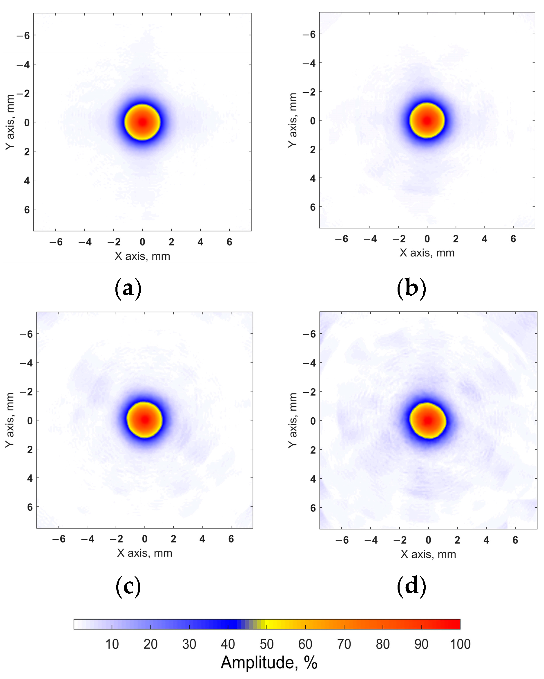
| Configuration | Defect | API | SNR | ||
|---|---|---|---|---|---|
| Value | Difference, % | Value, dB | Difference, dB | ||
| Full array | A | 0.623 | 0 | 36.21 | 0 |
| B | 0.649 | 0 | 33.89 | 0 | |
| C | 0.668 | 0 | 33.18 | 0 | |
| Sparse 49-element | A | 0.614 | 1.44 | 33.49 | −2.72 |
| B | 0.640 | 1.39 | 32.71 | −1.18 | |
| C | 0.670 | 0.30 | 30.68 | −2.5 | |
| Sparse 36-element | A | 0.620 | 0.48 | 32.61 | −3.6 |
| B | 0.661 | 1.85 | 29.67 | −4.22 | |
| C | 0.650 | 2.69 | 29.48 | −3.7 | |
| Sparse 25-element | A | 0.629 | 0.96 | 27.98 | −8.23 |
| B | 0.634 | 2.31 | 26.35 | −7.54 | |
| C | 0.645 | 3.44 | 26.83 | −6.35 | |
Disclaimer/Publisher’s Note: The statements, opinions and data contained in all publications are solely those of the individual author(s) and contributor(s) and not of MDPI and/or the editor(s). MDPI and/or the editor(s) disclaim responsibility for any injury to people or property resulting from any ideas, methods, instructions or products referred to in the content. |
© 2024 by the authors. Licensee MDPI, Basel, Switzerland. This article is an open access article distributed under the terms and conditions of the Creative Commons Attribution (CC BY) license (https://creativecommons.org/licenses/by/4.0/).
Share and Cite
Dolmatov, D.O.; Zhvyrblya, V.Y. Optimal Design of Sparse Matrix Phased Array Using Simulated Annealing for Volumetric Ultrasonic Imaging with Total Focusing Method. Sensors 2024, 24, 1856. https://doi.org/10.3390/s24061856
Dolmatov DO, Zhvyrblya VY. Optimal Design of Sparse Matrix Phased Array Using Simulated Annealing for Volumetric Ultrasonic Imaging with Total Focusing Method. Sensors. 2024; 24(6):1856. https://doi.org/10.3390/s24061856
Chicago/Turabian StyleDolmatov, Dmitry Olegovich, and Vadim Yurevich Zhvyrblya. 2024. "Optimal Design of Sparse Matrix Phased Array Using Simulated Annealing for Volumetric Ultrasonic Imaging with Total Focusing Method" Sensors 24, no. 6: 1856. https://doi.org/10.3390/s24061856