Impacts of Spatial Resolution and XCO₂ Precision on Satellite Capability for CO₂ Plumes Detection

Abstract

Greenhouse gas satellites can provide consistently global CO₂ data which are important inputs for the top-down inverse estimation of CO₂ emissions and their dynamic changes. By tracking greenhouse gas emissions, policymakers and businesses can identify areas where reductions are needed most and implement effective strategies to reduce their impact on the environment. Monitoring greenhouse gases provides valuable data for scientists studying climate change. The requirements for CO₂ emissions monitoring and verification support capacity drive the payload design of future CO₂ satellites. In this study, we quantitatively evaluate the performance of satellite in detecting CO₂ plumes from power plants based on an improved Gaussian plume model, with focus on impacts of the satellite spatial resolution and the satellite-derived XCO₂ precision under different meteorological conditions. The simulations of CO₂ plumes indicate that the enhanced spatial resolution and XCO₂ precision can significantly improve the detection capability of satellite, especially for small-sized power plants with emissions below 6 Mt CO₂/yr. The satellite-detected maximum of XCO₂ enhancement strongly varies with the wind condition. For a satellite with a XCO₂ precision of 0.7 ppm and a spatial resolution of 2 km, it can recognize a power plant with emissions of 2.69 Mt CO₂/yr at a wind speed of 2 m/s, while its emission needs be larger than 5.1 Mt CO₂/yr if the power plant is expected to be detected at a wind speed of 4 m/s. Considering the uncertainties in the simulated wind field, the satellite-derived XCO₂ measurements and the hypothesized CO₂ emissions, their cumulative contribution to the overall accuracy of the satellite’s ability to identify realistic enhancement in XCO₂ are investigated in the future. The uncertainties of ΔXCO₂ caused by the uncertainty in wind speed is more significant than those introduced from the uncertainty in wind direction. In the case of a power plant emitting 5.1 Mt CO₂/yr, with the wind speed increasing from 0.5 m/s to 4 m/s, the simulated ΔXCO₂ uncertainty associated with the wind field ranges from 3.75 ± 2.01 ppm to 0.46 ± 0.24 ppm and from 1.82 ± 0.95 ppm to 0.22 ± 0.11 ppm for 1 × 1 km² and 2 × 2 km² pixel size, respectively. Generally, even for a wind direction with a higher overall uncertainty, satellite still has a more effective capability for detecting CO₂ emission on this wind direction, because there is more rapid growth for simulated maximal XCO₂ enhancements than that for overall uncertainties. A designed spatial resolution of satellite better than 1 km and a XCO₂ precision higher than 0.7 ppm are suggested, because the CO₂ emission from small-sized power plants is much more likely be detected when the wind speed is below 3 m/s. Although spatial resolution and observed precision parameters are not sufficient to support the full design of future CO₂ satellites, this study still can provide valuable insights for enhancing satellite monitoring of anthropogenic CO₂ emissions.

1. Introduction

The Intergovernmental Panel on Climate Change (IPCC) notes that global greenhouse gas emissions have risen to an unprecedented level, with a linear increase in the average temperature of the global land and ocean surface [1]. The impacts of climate change have led to irreversible effects on agriculture, ecological systems, and terrestrial and marine environments. The Paris Agreement is committed to substantially reducing global greenhouse gases (GHGs) emissions with the objective of maintaining the global temperature increase within this century below 2 °C above pre-industrial levels, while pursuing effects to limit the temperature increase to 1.5 °C [2]. As the main component of atmospheric GHGs, carbon dioxide (CO₂) accounts for approximately 65% of the radiation forcing from long-lived GHGs [3]. In 2021, Human activities were responsible for the emission of about 37.12 billion metric tons of CO₂, predominantly from the combustion of fossil fuels in industrial processes [4]. Atmospheric CO₂ measured at NOAA’s Mauna Loa Atmospheric Baseline Observatory peaked for 2021 in May at a monthly average of 419 parts per million (ppm), the highest level since accurate measurements began 63 years ago, scientists from NOAA and Scripps Institution of Oceanography at the University of California San Diego announced today. Emission hot spots, such as megacities, large steel producing factories, volcanoes, and power plants, are major contributors to global energy-related CO₂ emissions [5,6]. Compared to other point sources, power plants are more representative, power plants contribute a significant portion of global greenhouse gas emissions. They have continuous emission durations, stable emission rates, and emissions that are more concentrated. Additionally, monitoring the emission rates of power plants is already well-established, with emission inventories providing emission rate information. Although all are considered point sources of emissions, power plants better fit the theoretical definition of a point source. Consequently, the quantification and routine update of global CO₂ emissions of these hot spots are crucial for the international climate negotiations focused on carbon emission reduction.

The top-down and bottom-up approaches are two primary methodologies of CO₂ emission estimation. The bottom-up approach provides detailed information on individual sources, whereas the top-down approach yields more general information on overall emissions. Bottom-up CO₂ emission inventories are often subject to significant uncertainties due to reasons such as the limitations in data availability and adequacy, as well as the techniques employed in data processing. With the development of GHG satellites in recent years, space-based observations are increasingly used for the top-down inverse estimation of CO₂ emission. This approach estimates regional carbon sources and sinks and their dynamic changes by combining atmospheric observations of greenhouse gas concentrations and meteorological data with atmospheric chemical transport models through complex data assimilation methods. Satellite observations have an advantage over ground-based measurements by providing comprehensive and consistent atmospheric CO₂ data for both terrestrial and marine surfaces on a global scale. Presently, numerous countries are committed to developing global or regional Monitoring and Verification Support (MVS) systems for anthropogenic CO₂ emissions, in alignment with the Paris Agreement of the United Nations Framework Convention on Climate Change (UNFCCC). These MVS systems are designed to enhance the accuracy of national greenhouse gas emissions inventories, particularly through top-down verification of emissions using globally high spatial and temporal resolution observations from space-based sensors [5,6,7]. For instance, a European Commission (EC) expert panel raised high-level requirements that have been translated into technical requirements, proposing technical specifications for satellite sensors with clearly defined spatial and temporal resolutions and emission source monitoring capabilities [3].

Several countries, including Japan, the United States, and China, have launched GHG satellites [8,9,10,11,12]. The Greenhouse Gases Observing Satellite (GOSAT) as Japan’s pioneering GHG satellite was launched in January 2009. It was designed to monitor the global distributions of CO₂ and CH₄ from space and remains operational. As a successor mission of GOSAT, GOSAT-2 equipped with the improved TANSO-FTS-2 featuring enhanced signal-to-noise ratio (SNR), was launched in October 2018. Both GOSAT and GOSAT-2 employ non-consecutive sampling, cross-track mechanical pointing, which restrict their observational spatial coverage (swath 790 km, 10.5 km at sub-satellite point) [13]. Launched in July 2014, Orbiting Carbon Observatory-2 (OCO-2) is an Earth observing satellite mission owned and operated by National Aeronautics and Space Administration (NASA). The OCO-2 instrument utilizes a pushroom scanning technique with a swath width of 10 km and spatial resolution of 1.29 km cross-track and 2.25 km along-track [14]. In December 2016, China successfully launched its first GHG observation satellite, TanSat. OCO-2 and Transat use continuous pixel observations facilitated by high-resolution raster spectroscopy, enabling monitoring CO₂ emissions from point sources [15]. However, due to their narrow swath widths (10~25 km) and revisit periods, there is a notable observational gap area between their orbital paths, limiting their ability to capture temporal variability of emissions from sources like power plants [16]. OCO-3, installed on the International Space Station (ISS) in May 2019, introduced Snapshot Area Map mode, targeting specific areas approximately 80 × 80 km², such as fossil fuel emission sources, volcanoes, and field validation sites. Through multiple observations of the same power plant by OCO-3, this mode assists in quantifying complex emission sources [5,17]. Above operational satellites (GOSAT, GOSAT-2, OCO-2, OCO-3 and TanSat) represent the first generation of CO₂ satellite missions, primarily focused on obtaining global CO₂ distribution. By using long time-series XCO₂ monitored by these satellites, it can offer insights into continental-scale CO₂ budgets and initial understanding of the carbon flux in land surface systems [17,18,19,20]. Atmospheric CO₂ concentration has been examined in several studies from different perspectives, such as spatial distribution and relation with different variables and so on [13,21,22,23]. While the detection accuracy of these satellites has improved to a certain level, their overall capabilities remain limited [6,24], particularly in terms of coverage range and spatial-temporal resolution. Therefore, in view of the technical shortcomings of the first generation of carbon satellites, the detection capability of the next generation of carbon satellites needs to be improved, and not only the spatial and temporal resolution, but also the coverage range.

To meet the requirements for CO₂ emissions monitoring and verification support capacity, the next-generation CO₂ satellites is being conceptualized and developed by the European Union (EU), Japan, the United States, China, and so on. The Copernicus Anthropogenic Carbon Dioxide Monitoring (CO2M), as a part of the EU’s Copernicus Sentinel Expansion mission, is specifically designed to quantify CO₂ emissions attributable to human activities. Planned for launch in 2025, CO2M aims to enhance our understanding of anthropogenic CO₂ release. Meanwhile, China is progressing with its next-generation CO₂ satellite mission, which is currently undergoing a rigorous evaluation of satellite platform and payloads designing. The next-generation CO₂ satellites are tasked with reducing current uncertainties in estimation of CO₂ emissions from fossil fuel combustion at both national and regional levels. Given the rapid dilution of CO₂ after emission, further satellites are expected to possess enhanced capabilities for frequent and comprehensive capture of entire CO₂ plumes with high single-sounding precision [25]. These above requirements translate into needs for the XCO₂ retrieval precision, spatial sampling, spatial resolution, and global coverage. These prerequisites further drive the design of satellite instruments, particularly concerning SNR, as well as spatial co-registration and spectral stability. Such developments are essential for achieving the desired accuracy and efficiency in CO₂ emission monitoring and verification at a global scale.

For the next-generation CO₂ satellite missions design, two pivotal observational characteristics for detecting plumes from coal-fired power plants are spatial resolution and the precision of satellite-derived XCO₂ measurements. The detectable signal of enhanced XCO₂ also depends on the wind field due to the rapid dispersion of CO₂ post-emission. In this study, the Gaussian plume model method was used to simulate and analyze the CO₂ diffusion under a variety of atmospheric conditions and for different emission sources, considering the impact of varying pixel sizes on satellite monitoring effectiveness. Section 3 presents a quantitative analysis of the relationship between spatial resolution and satellite monitoring capability for terrestrial CO₂ emission sources under different atmospheric conditions and emission intensities. In Section 4, we explore and discuss the effects of the simulated wind field, satellite-derived XCO₂, and hypothesized CO₂ emission on the overall uncertainty of realistic XCO₂ enhancements which can be identified by satellite. Although the results of this study alone are not definitive in determining the design architecture of future CO₂ monitoring satellites, they provide valuable insights that may guide the development of space-based systems for monitoring anthropogenic CO₂ emissions.

2. Methods

2.1. Simulation Region

In this study, to assess the efficacy of satellite-based monitoring of CO₂ emissions from power plants, simulations were conducted to analyze XCO₂ enhancements under different scenarios within a defined area of 60 × 60 km². This designated region was subdivided into 50 m × 50 m grids for the generation of realistic CO₂ plume simulations. The XCO₂ enhancement data derived from these simulations were further averaged across these grid-generated CO₂ plume images. To mimic satellite observations, these data were further utilized to create downscaled square tiles, simulating satellite observation images at spatial resolutions of 0.5 × 0.5 km², 1 × 1 km², 2 × 2 km², and 4 × 4 km². Uncertainties in the XCO₂ enhancement identified by satellite were statistically analyzed. This analysis considered various factors, including meteorological conditions, CO₂ emissions and satellite noises, to evaluate the precision and reliability of satellite observations in monitoring atmospheric CO₂ levels.

2.2. Gaussian Plume Model

Currently, the Gaussian plume model is mainly used for estimating the emission of a single power plant using satellite observations of XCO₂ [15,26]. For the simulation of XCO₂ enhancement above the background concentration, an advanced version of the Gaussian plume model was adopted in this study [27], specifically an improved vertically integrated Gaussian plume model. This refined model is predicated on a series of slightly modified equations used by Bovensmann et al. [28]. These modifications enhance the model’s accuracy and applicability in simulating the dispersion of XCO₂ in the atmosphere, providing a more precise representation of CO₂ plume behavior.

$$V(x,y)=\frac{F}{\sqrt{2\pi }{\sigma }_y(x)\mu }{e}^{-\frac{1}{2}{(\frac{y}{{\sigma }_Y(x)})}^2}$$

(1)

$${\sigma }_y(x)=a{(\frac{x}{x_0})}^{\gamma }$$

(2)

where V (x, y) is the CO₂ vertical column density (in g/m²) at coordinates (x, y). Here, x (in m) denotes the downwind distance from the point source, and y (in m) is the distance perpendicular to the wind. The orientation of x is parallel to the wind direction, and the orientation of y is perpendicular to the wind direction. The wind direction (θ) is measured counterclockwise from the eastward direction to the along-track direction of satellite. V (x, y) can be calculated from CO₂ emission rate (F, in g/s), wind speed (μ, in m/s), and the standard deviation in the y direction (σ_y(x), in m) which determines the rate of diffusion perpendicular to the wind. a (in m) is the atmospheric stability parameter, determined based on the Pasquill–Gifford stability classification [29,30]. Here, a is depending on Pasquill stability classes, which can be determined from the 10 m wind speed and solar radiation. a is empirically set at different values based on wind speed: a = 213 m for μ < 2 m/s, either a = 213 or 156 m for 2 m/s ≤ μ < 3 m/s, a = 156 m for 3 m/s ≤ μ < 5 m/s, and a = 104 m for μ > 5 m/s [29,30]. Additionally, the previous Gaussian dispersion model did not consider the influence of crosswind diffusion when calculating σ_y(x). Therefore, later scholars added crosswind diffusion to the original formula, namely: x₀ = 1000 m, where x₀ is defined as the characteristic length representing crosswind diffusion. The parameters set in the formulas are only for the simulation of plume dispersion in the next-generation carbon satellite. These parameters are universal, but meteorological factors in actual pollution processes are constantly changing. Therefore, the results simulated using the parameters set in the document may not fully represent the complete pollution dispersion process under real conditions.

Then, the enhancement of XCO₂, quantified in parts per million (in ppm), is derived from V (x, y) based on the following equation [26,31]:

$$XC{O}_2=V(x,y)·\frac{M_{air}}{M_{C{O}_2}}·\frac{g}{P_{surf}-w·g}·1000$$

(3)

where M_air, M_CO2, and g are three constants. M_air and M_CO2 represent the molecular weights (in kg/mol) of air and CO₂, respectively. And g denotes the gravitational acceleration (in m/s²). P_surf refers to the surface pressure (in Pa), and w signifies the total column water vapor (in kg/m²).

The background wind field in this study is assumed to be stable and uniform, ensuring that the XCO₂ distribution adheres to a normal distribution pattern throughout the continuous point source diffusion process. It is important to note that the CO₂ plume is considered only in terms of horizontal dispersion, with turbulent diffusion along the wind direction (θ) being disregarded, and the vertical diffusion of the plume being ignored. Therefore, the influence of terrain effects on plume dispersion was not considered.

2.3. Uncertainties Estimation

The capacity of satellites to detect CO₂ plumes emitted from point sources, such as power plants, is intrinsically related to several key factors: the simulated wind field, the satellite-derived XCO₂ measurements, and the hypothesized CO₂ emissions. Point source emissions dispersion is greatly influenced by wind. Wind speed affects the speed of pollutant spread, while wind direction affects the direction of pollutant spread. The plume enhancement results captured by satellites include errors inherent to the satellites themselves, which can impact the plume enhancement results to a certain extent. The assumed CO₂ emission results come from ground monitoring devices, which have their own monitoring errors, leading to errors in CO₂ emission estimates. Consequently, the uncertainties or errors inherent in these three factors cumulatively contribute to the overall accuracy of the satellite’s ability to identify realistic enhancement in XCO₂. This overall uncertainty plays a pivotal role in determining the reliability and precision of satellite-based observations in recognizing atmospheric CO₂ variations.

Through tuning parameters such as wind speed, wind direction, satellite-derived XCO₂ error, and the uncertainty of CO₂ emission from the power plant, the overall uncertainty in satellite-detected XCO₂ enhancement (denoted as ε) can be quantitatively determined by

$$\epsilon =\sqrt{{\epsilon }_w^2+{\epsilon }_s^2+{\epsilon }_e^2}$$

(4)

where ε_w represents the simulated uncertainty associated with the wind field, which is determined as the standard deviation derived from incorporating uncertainties into both wind speed and wind direction for plume simulation. ε_s is attributed to the error in satellite-based XCO₂ led by the instrument noise and the model error of XCO₂ retrieval. Furthermore, ε_e is the discrepancy of CO₂ emissions, contrasting the statistical data from “bottom-up” CO₂ emission inventory with the actual emission values. ε is the total error then determined from the wind, instrument noise, and CO₂ emissions.

Here, ε_w can be calculated by

$${\epsilon }_w=\sqrt{{\epsilon }_w^2\left(\mu \right)+{\epsilon }_w^2\left(\theta \right)}$$

(5)

where ε_w(μ) and ε_w(θ) are the uncertainties in XCO₂ introduced by wind speed and wind direction, respectively.

3. CO₂ Plume Simulation and Analysis

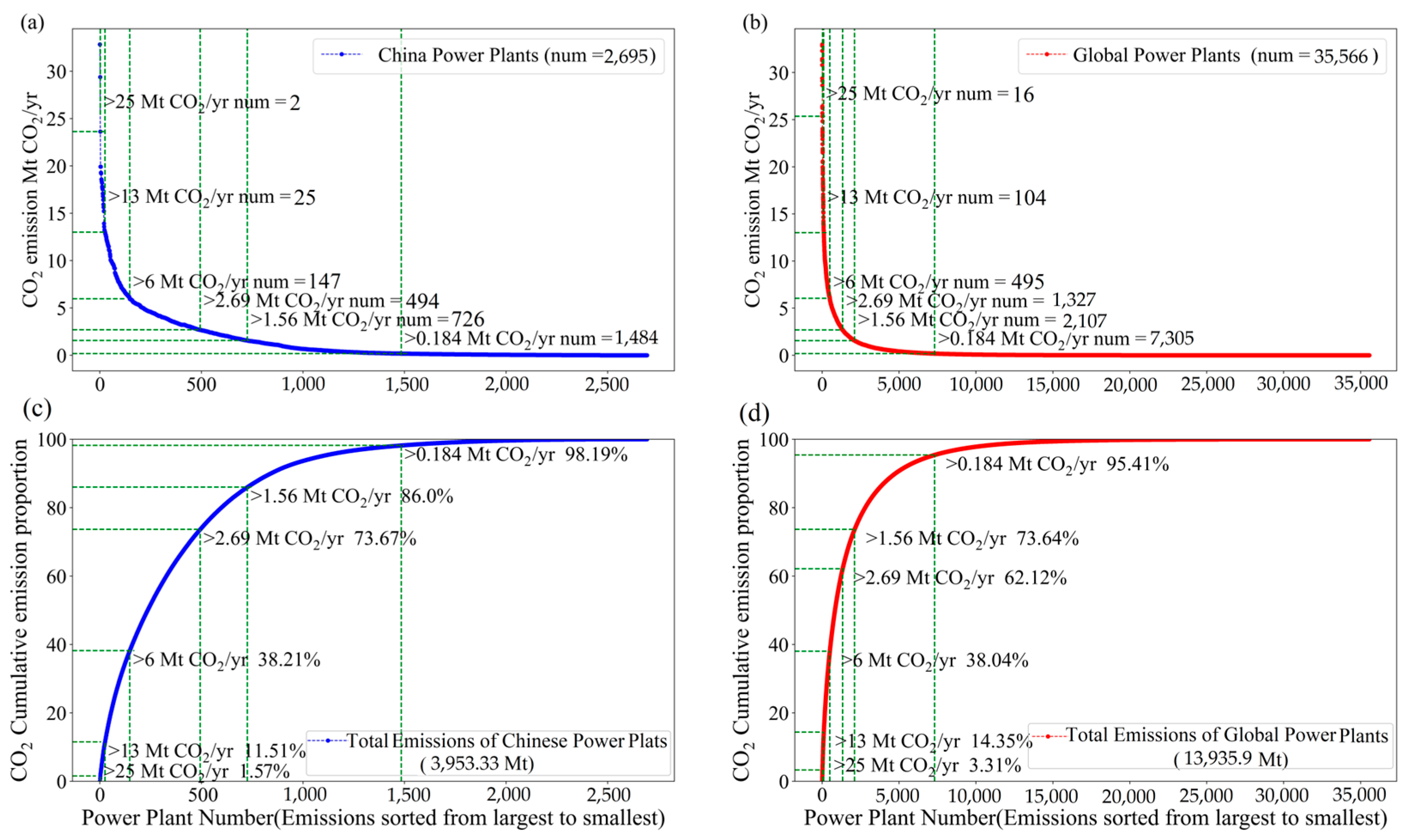
3.1. CO₂ Emission from Plant Power

As the most important point source, CO₂ emissions from power plants constitute a significant portion of global anthropogenic CO₂ sources. In order to evaluate the satellite detection capability of power plants around the world and China, the global power emissions database (GPED) v1.1 was used for counting the CO₂ emission ratio of the satellite-detected amount to the total amount from power plants. GPED is a publicly available bottom-up emission inventory including global plant-level CO₂ emission data of power plants across all countries [32]. Analysis of 2019 emission statistics from GPED v1.1, as illustrated in Figure 1, reveals that power plants with CO₂ emissions of more than 0.184, 6, 13 and 25 Mt CO₂/yr comprise only 20.53%, 13.91%, 0.29% and 0.04% of the global total count, yet their cumulative emissions account for 95.41%, 38.04%, 14.35% and 3.31% of the total amount of CO₂ emission from global power plants, respectively. In the context of China, power plant emissions over 0.184, 6, 13 and 25 Mt CO₂/yr correspond to 55.06%, 5.45%, 0.92% and 0.07% of the total number, contributing 98.19%, 38.21%, 11.51% and 1.57% of the country’s total CO₂ emission, respectively. Here, the reference CO₂ emission level of 0.184 Mt CO₂/yr is one of the high-level policy needs to develop the MVS capacity for anthropogenic CO₂ emissions in the EU, as proposed by Pinty et al. [33]. Furthermore, according to previous studies, emission levels of 6, 13 and 25 Mt CO₂/yr can be employed to categorize low-, medium- and high-sized power plants, respectively [15].The emission rates of power plants in reality are subject to variations due to hardware and external factors, and are not constant. This article simply uses constant emission rates for plume simulation under ideal conditions.

3.2. Detection Capability of Satellite with Different Spatial Resolutions and XCO₂ Precisions

To assess the performance of satellite in the detection of CO₂ plumes from power plants with different CO₂ emission intensities, 6, 13, and 25 Mt CO₂/yr were converted to CO₂ emission rate F to represent the low, medium, and high emission level of point sources, respectively. μ = 4 m/s, a = 156.0 m, θ = 45° were set for the simulation of CO₂ plume over a domain with a pixel size of 0.5 × 0.5 km². Based on existing research findings and the latest XCO₂ measurement results, the background concentration of XCO₂ in this experiment is set to 420 ppm. This value represents an idealized state and is considered universally applicable, without accounting for regional variations. It is solely used for simulating payloads for the next-generation carbon satellite.

Additionally, the space-based XCO₂ error caused by instrument noise and retrieval algorithm is also a primary limitation in the detection of CO₂ plumes. The XCO₂ monitoring precision for the first-generation CO₂ satellites (e.g., GOSAT, GOSAT-2, OCO-2 and Tansat) is ~1.5 ppm [8]. In contrast, the next-generation CO₂ satellites (e.g., CO2M and Tansat2) aim for a more stringent XCO₂ precision of ~0.7 ppm. Noise was superimposed over the simulated enhancements to represent random errors that would occur in true observations. The noise or random error was generated following a normal distribution. Here, to simulate realistic satellite observations with different spatial resolutions, gaussian errors of 0.7 and 1.5 ppm (i.e., ε_s) were added to generate simulated images of satellite observation with different spatial resolutions. The outcomes of these simulations, showcasing the impact of these errors on observational accuracy at different spatial resolutions, are depicted as shown in Figure 2.

According to the simulated XCO₂ enhancement results, it is indicated that for the power plant with low-level emission of 6 Mt CO₂/yr, identifying the emitted CO₂ plume becomes challenging when the spatial resolution is coarser than 1 km. This is primarily because the XCO₂ enhancement from emission is either smaller than or comparable to the XCO₂ error from satellite observation. A notable increase in the capability to detect CO₂ plumes from space is shown when the ε_s is reduced from 1.5 ppm to 0.7 ppm. For satellites with an ε_s of 1.5 ppm, the substantial noise interference significantly weakens the CO₂ plume signal, making it discernible only for emission sources with 25 Mt CO₂/yr at pixel sizes of 0.5, 1 and 2 km. However, for ε_s = 0.7 ppm, power plants emitting more than 13 Mt CO₂/yr emission can be effectively detected by satellite through clearly observable CO₂ plumes at spatial resolutions of 4 km or higher. Even though a distinct shape of CO₂ plume may not be obtained for a simulation region with 1 × 1 km² and lower emission rates, a remarkable XCO₂ enhancement in several specific pixels proximal to the emission source can still be detected by satellite with an ε_s = 0.7 ppm. And such isolated pixels characterized by abnormally high XCO₂ values also have potential for estimating CO₂ emissions from point sources through multiple repeat observations by satellite. Therefore, compared with the first-generation CO₂ satellites, the indicator improvement in XCO₂ precision will enhance the detection of the CO₂ emission plumes and isolated high-level XCO₂ pixels for the next-generation CO₂ satellites, thereby benefiting the capturing of point source emissions. The set satellite monitoring precision and the simulated plume dispersion results at different spatial resolutions in this study are all aimed at meeting the observation requirements of the next-generation carbon satellite. These simulations serve as a forward simulation for determining satellite payload indicators.

To investigate the detection capability of satellite more quantitatively for CO₂ emissions from small- and medium-sized power plants (emissions < 15 Mt CO₂/yr), we conducted a series of plume simulations with a 2 × 2 km² pixel size. These CO₂ plume simulations were generated by changing CO₂ emissions in a range of 0~15 Mt CO₂/yr with a step of 0.1 Mt CO₂/yr. Here, taken 2 × 2 km² as a standard value, the main reason is that 2 km is the designed spatial resolution of both CO2M and Tansat2. As shown in Figure 3, under conditions of μ = 4 m/s and θ = 270°, if the maximum values of XCO₂ enhancement (donated as ΔXCO2_max) in the simulation domain reach up to 0.5, 0.7, 1.0 and 2.0 ppm, the source emissions need to be larger than 3.6, 5.1, 7.3 and 14.5 Mt CO₂/yr, respectively. It is indicated that the ε_s of satellite should be less than 0.5, 0.7, 1.0 and 2.0 ppm, so that the XCO₂ enhancements generated by power plants with an emission of 3.6, 5.1, 7.3 and 14.5 Mt CO₂/yr can be detected, respectively. In addition, considering that power plants with emissions larger than 1.56 or 2.69 Mt CO₂/yr contribute ~85% and ~75% to the total emissions of global power plants based on GPED (Figure 1), emission levels of 1.56 and 2.69 Mt CO₂/yr were also selected as reference emission thresholds with the other four values mentioned above in Section 3.1.

Based on the simulations depicted in Figure 3, satellites with higher spatial resolution can better identify point sources with lower emissions under the same conditions. However, achieving the aim of 0.184 Mt CO₂/yr is still very difficult to realize for space-based instruments with medium spatial resolution. For instance, even for a pixel size of 0.5 × 0.5 km², the ε_s needs be lower than 0.11 ppm if the emitted CO₂ plume or XCO₂ enhancement pixel can be detected by satellite. A notable improvement in detection capabilities is observed when the designed spatial resolution of satellite is enhanced from 2 km to 1 km. Specifically, the ΔXCO2_max values increase by ~0.5, ~0.7, ~1.1 and ~2.2 ppm for emissions of 3.6, 5.1, 7.3 and 14.5 Mt CO₂/yr, respectively. For a satellite with an ε_s of ~1 ppm and spatial resolutions of 2 km, 1 km, or 0.5 km, it could potentially detect power plants with emissions of 7.3, 3.6 or 1.56 Mt CO₂/yr, respectively. But for a satellite with a spatial resolution of 4 km, it can only detect large-sized power plants with CO₂ emissions exceeding 14.5 Mt CO₂/yr.

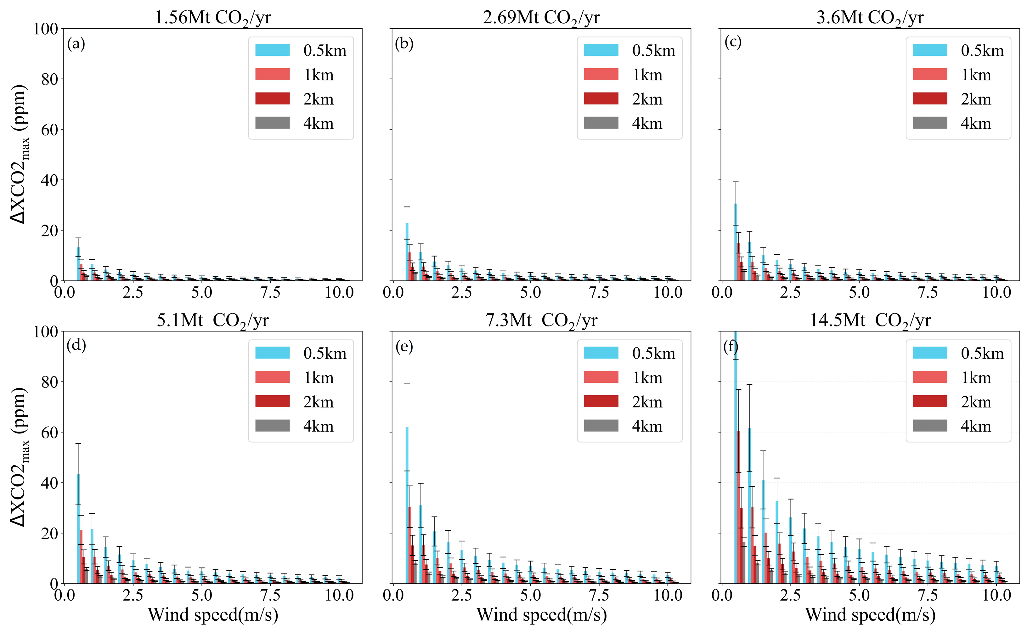
3.3. Detection Capability of Satellite under Different Wind Field Conditions

Compared with power plant emission and satellite-derived XCO₂ precision which are considered relatively stable factors, the wind field exhibits continuous temporal and spatial variability. During the diffusion process of CO₂ plume, the wind speed not only affects the propagation speed of the plume but also has an impact on the XCO₂ gradient within the plume. Consequently, for a relatively fixed CO₂ emission rate of the power plant, whether the emitted CO₂ plume can be identified by satellite mostly depends on both the instantaneous wind speed and wind direction. As shown in Figure 4 and Figure 5 which are similar to Figure 3 with different wind speed and wind direction, the ΔXCO2_max varies from 0.23 to 13.18 ppm for a certain parameter set of CO₂ emission level and satellite spatial resolution. With an increased emission amount and satellite spatial resolution, the impact of wind field on the variation of ΔXCO2_max tends to become stronger. As for a spatial resolution of 2 km and a fixed θ of 270°, the ΔXCO2_max increases by 0.19 to 1.78 ppm as the μ decreases from 4 m/s to 2 m/s. Similarly, altering the θ from 270° to 45°, results in the ΔXCO2_max increase by 0.32~3.02 ppm for a fixed μ of 4 m/s. For a satellite with an ε_s of 0.7 ppm and a spatial resolution of 2 km, it can distinguish a power plant with emission of 5.1 Mt CO₂/yr from the background noise (as shown in Figure 3) at a μ of 4 m/s, but its detection capability can be enhanced to 2.69 Mt CO₂/yr when the μ decreases to 2 m/s.

In order to explore the relationship between the wind field and the satellite capability for the CO₂ plume detection, XCO₂ distribution and ΔXCO2_max were calculated by varying the μ from 0.5 m/s to 10 m/s in increments of 0.5 m/s and the θ from 0° to 360° in increments of 15°. Based on the statistics data of ΔXCO2_max in Figure 6, ΔXCO2_max is inversely proportional to both satellite spatial resolution and μ. ΔXCO2_max rapidly reduces with μ increasing for μ within the range of 1.5 and 5 m/s, while this downward trend slows down for μ greater than 5 m/s. Figure 7 presents the mean and standard deviation results of ΔXCO2_max from XCO₂ distribution simulations, displayed in polar coordinates for a fixed θ across varying μ values. And the concentric rings, from inner to outer, correspond to the ΔXCO2_max simulations for emission levels of 1.56, 2.69, 3.6, 5.1, 7.3 and 14.5 Mt CO₂/yr, respectively. The results indicate that for the wind directions at 45°, 135°, 225° and 315°, both the means and standard deviations of ΔXCO2_max are significantly larger than those for the wind directions at 0°, 90°, 180° and 270°. The main reason is that a greater number of valid 50 m × 50 m grids containing high XCO₂ data within the CO₂ plume image is involved in calculating averaged XCO₂ enhancements when θ is set to 45°, 135°, 225° or 315°.

Figure 8 describes the variation in ΔXCO2_max with the increase in μ for different power plant emission levels and satellite spatial resolutions. The error bars are corresponding to the standard deviations of ΔXCO2_max for all θ values ranging from 0° to 360° in 5°increments, within each binned μ category. For small-sized power plants (emissions < 6 Mt CO₂/yr) and a pixel size of 2 × 2 km², the variation in ΔXCO2_max among different wind directions is very small (<1 ppm) when the μ is larger than 3 m/s, and such difference declines as the wind speed increases. However, for the μ below 1.5 m/s, the difference in ΔXCO2_max among different wind directions can reach up to about 4 to 8 ppm. The ΔXCO2_max standard deviation increases for the power plants with higher emission levels (e.g., mid-sized power plants), meaning a strong impact of wind direction on the ΔXCO2_max. Due to the positive correlation between the pixel size and the satellite-detected ability of CO₂ plume, this trend is further accentuated for smaller pixel sizes, such as 0.5 km and 1 km, where a remarkable growth appears in the ΔXCO2_max standard deviation is observed. Therefore, both wind speed and wind direction are critical parameters which can introduce large uncertainty into CO₂ emission estimation by using satellite-derived XCO₂, especially for power plants at medium/high emission levels.

4. Uncertainty Analysis

4.1. Impact of the Uncertainty in Wind Field

Here, a 10% uncertainty was assumed for both wind speed and wind direction which can be obtained from atmospheric reanalysis or numerical weather prediction data [34]. The uncertainty of the wind field ε_w is quantified as the standard deviation of the ΔXCO2_max variation, which was calculated by separately adding a random error of 10% in both wind speed and wind direction for each plume simulation. The parameters used for these CO₂ plume simulations were consistent with those in Section 3.3, ensuring uniformity and comparability across the study.

The uncertainties of satellite-detected XCO₂ enhancement led by errors of wind field under scenarios of θ = 45° and 270° are shown in Figure 9 and Figure 10, respectively. Generally, compared to the impact of ε_w(θ), ε_w(μ) plays a dominant role in the variation of ε_w for both θ = 45° and 270°. And the uncertainties of ΔXCO₂ caused by the uncertainty in wind speed is more significant than those introduced from the uncertainty in wind direction. Under a condition with the same wind speed and emission level, there is a significant difference in ε_w(μ) and ε_w between θ = 45° and θ = 270° scenarios, while the ε_w(θ) at θ = 45° is similar to that at θ = 270°. For example, in the case of a small-sized power plant with a CO₂ emission of 5.1 Mt CO₂/yr, ε_w(μ) values vary in the range of 0.36~2.80 ppm and 0.17~1.37 ppm for satellite pixel sizes of 1 × 1 km² and 2 × 2 km², respectively, with θ = 45° and μ ranging from 0.5 to 4 m/s. Under the same conditions yet at θ = 270°, ε_w(μ) only spans from 0.13 to 1.06 ppm and 0.06 to 0.53 ppm for the satellite with spatial resolutions of 1 km and 2 km, respectively. In comparison with ε_w(μ), ε_w(θ) is smaller and its variation is more stable. And the ε_w(θ) values at both θ = 45° and 270° are all less than 0.5 ppm. As for the overall uncertainty of ΔXCO₂ arising from both wind speed and wind direction, the maximum difference in ε_w between θ = 45° and θ = 270° is approximately 2.5 times under conditions of point sources emitting less than 6 Mt CO₂/yr, μ below 2 m/s and spatial resolution coarser than 1 km. Taking the power plant with CO₂ emission of 5.1 Mt CO₂/yr at μ = 0.5 m/s as an example, ε_w values at θ = 45° reach up to 2.81 and 1.37 ppm corresponding to satellite spatial resolution of 1 km and 2 km, respectively, whereas they are only 1.09 and 0.54 ppm for θ = 270°. When the μ increases to 4 m/s under these conditions, there is a significant decline in ε_w. These results at θ = 45° are 0.36 and 0.17 ppm for 1 km and 2 km spatial resolutions, respectively, and are 0.14 and 0.06 ppm at θ = 270°. Such difference grows with increasing emission rates from the point source and decreases with rising wind speeds.

To comprehensively investigate the influence of uncertainties in wind speed and wind direction on satellite detection of CO₂ plumes, simulations similar to those in Figure 9 and Figure 10 were extended to θ ranging from 0° to 360° with intervals of 15°. Figure 11a and Figure 11b are the means (ε_w,mean) and standard deviations (ε_w,std) of ε_w values across all wind directions, respectively, for different wind speeds, pixel sizes and emission levels. Both ε_w,mean and ε_w,std are directly proportional to the CO₂ emission rate of the power plant, while inversely correlating with the spatial resolution of satellite. For a point source emitting 5.1 Mt CO₂/yr, the ε_w decreases from 3.75 ± 2.01 ppm (expressed as ε_w,mean ± ε_w,std) to 0.46 ± 0.24 ppm with μ increasing from 0.5 m/s to 4 m/s for a pixel size of 1 × 1 km². Similarly, ε_w reduces from 1.82 ± 0.95 ppm to 0.22 ± 0.11 ppm when the pixel size is downscaled to 2 × 2 km². Figure 11c and 11d illustrate the maximums (ε_w,max) and minimums (ε_w,min) of ε_w across all wind speeds in the range of 0.5~10 m/s for a satellite spatial resolution of 2 km on different wind directions, respectively, where ε_w,max = ε_w,mean + ε_w,std and ε_w,min = ε_w,mean-ε_w,std. The results indicate a more significant difference in ε_w,max compared to that of ε_w,min among different wind directions. For a small-sized power plant with a CO₂ emission of 5.1 Mt CO₂/yr, the ε_w,max across wind directions from 0° to 360° varies from 0.21 ppm to 1.56 ppm with an average of 0.71 ppm, and the ε_w,min ranges only from 0.02 ppm to 0.15 ppm with an average of 0.08 ppm. As the emission rate of the power plant increases, the range of variability also increases. For a large-sized power plant with a CO₂ emission of 14.5 Mt CO₂/yr, the ε_w,max spans from 0.61 ppm to 4.45 ppm, averaging 2.03 ppm, and the ε_w,min ranges from 0.05 to 0.47 ppm, averaging 0.2 ppm.

4.2. Impact of the Uncertainty in CO₂ Emission Level

Developed and developing countries are gradually adopting continuous emission monitoring systems (CEMS) to monitor the real-time carbon emissions from thermal power plants, in order to obtain accurate, complete, and timely emission data. CEMS data are also uncertain, but we assume that those uncertainties are small, i.e., <10% [35,36]. Similar to the analysis of ε_w, an uncertainty of 10% was assumed for the CO₂ emission from power plants. Therefore, ε_e results were calculated by introducing a random error of 10% into the CO₂ emission rate for each plume simulation. The ε_e variations were further examined under different wind speeds and wind directions, as shown in Figure 12. Figure 12a and Figure 12b give the means (ε_e,mean) and standard deviations (ε_e,std) of ε_e values at all wind directions, respectively, for various wind speeds, pixel sizes and emission levels. The variability in ε_e among different wind directions is obvious only at low wind speeds. For instance, for a pixel size of 1 × 1 km², the ε_e varies from 0.11 ± 0.03 ppm to 6.04 ± 1.63 as the μ decreases from 3 m/s to 0.5 m/s, while it correspondingly ranges from 0.05 ± 0.01 ppm to 3.00 ± 0.8 ppm for 2 × 2 km². The maximums (ε_e,max) and minimums (ε_e,min) of ε_e under all scenarios with μ between 0.5 to 10 m/s are shown in Figure 12c and 12d, respectively, for a satellite spatial resolution of 2 km. The results reveal that the ε_e variability due to different wind speeds is closely related to wind direction and exhibits strong regularity. Both ε_e,max and ε_e,min values are relatively small, with ε_e,max and ε_e,mmin results of different CO₂ emission levels below 1.55 ppm and 0.5 ppm, respectively.

4.3. Estimation of Overall Uncertainty

The overall uncertainties in satellite-detected XCO₂ enhancement were derived using Equation (4). Here, the satellite-based XCO₂ error, ε_s, were set at varying levels of 0.5, 0.7, 1.0 and 1.5 ppm. The calculations of ε_w and ε_e correspond to the results in Section 4.1 and Section 4.2, respectively. The overall uncertainties ε with different ε_s values under conditions of θ = 45° are shown in Figure 13a–d, and results for θ = 270° are correspondingly depicted in Figure 14a–d. The variation trend of ε influenced by changes in wind speed, CO₂ emission level and satellite pixel size are similar for both θ = 45° and θ = 270°, but ε calculated for θ = 45° is larger than that for θ = 270° under the same scenario. The wind field significantly influences the variation of ε. Specifically, for an ε_s = 0.7 ppm and a power plant with an emission of 5.1 Mt CO₂/yr, ε simulations on 1 × 1 km² grids vary in the range of 0.74~4.0 ppm with an average of 1.09 ppm when θ = 45° and μ ranging from 0.5 to 4 m/s. And ε results range in the range of 0.70~2.0 ppm with an average of 0.83 ppm for 2 × 2 km² pixel size. On the wind direction of 270°, the ε range for a 1 × 1 km² pixel size is 0.7 to 1.67 ppm, averaging 0.79 ppm, and for a spatial resolution of 2 km, it is 0.70 to 1.03 ppm, averaging 0.72 ppm. When the wind speed is larger than 4 m/s, ε is almost constant for a pixel size bigger than 2 × 2 km².

To further investigate the performance of satellite in detecting CO₂ plumes from power plants with different CO₂ emissions, results of ΔXCO2_max subtracted from ε were analyzed, as shown in Figure 13e–h and Figure 14e–h. Here, blue regions represent the overall uncertainty less than ΔXCO2_max, meaning that satellite can detect the signal of XCO₂ enhancements generated by power plant emissions. White and light red regions suggest a reduced likelihood of satellite detection for CO₂ emission plumes. The detection capability of satellite under θ = 45° is proved more effective than that under θ = 270°. Generally, it is easier for satellite to detect XCO₂ enhancements when wind speed is below 3 m/s, particularly for medium- and large-sized power plants. In order to capture the CO₂ emission from small-sized power plants, the spatial resolution of the satellite should be better designed to be finer than 1 km. The probability of detecting CO₂ plume significantly decreases as the pixel size increases, and it depends to a large extent on the meteorologic condition.

5. Summary

The spatial resolution and the precision of satellite-derived XCO₂ measurements are two key indicators for the payload design of the next-generation CO₂ satellite missions, which decide the satellite’s capability in detecting CO₂ emissions. In this paper, by using the high-resolution Gaussian model, we focused on the simulation and uncertainty factors in satellite detection of CO₂ emissions from power plants on different conditions of satellite pixel sizes, satellite-derived XCO₂ errors and CO₂ emission levels. According to our simulations, detailed conclusions on the detection capabilities of satellites and their associated uncertainties in monitoring CO₂ plumes are found:

(1)

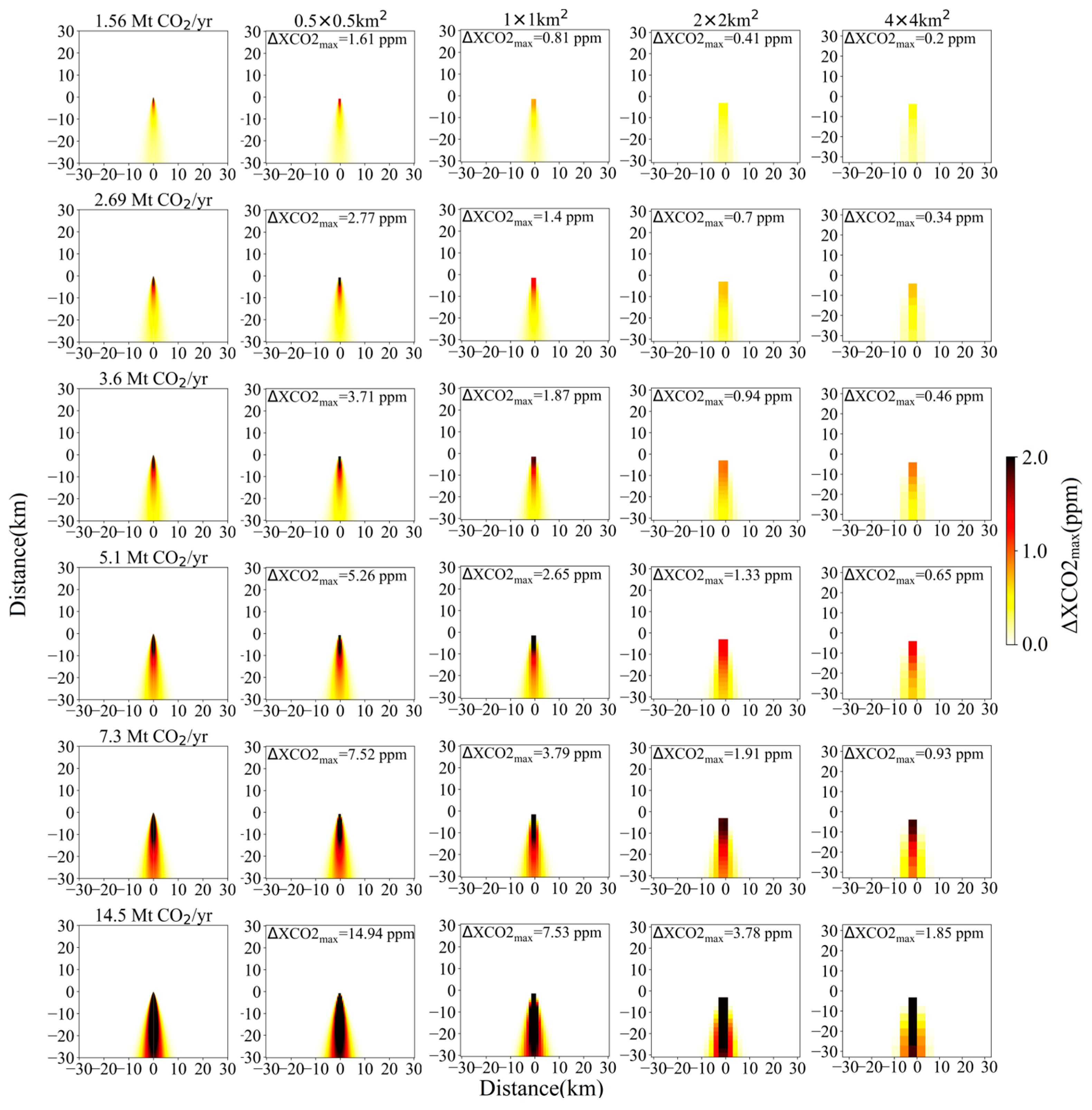
Generally, enhanced spatial resolution of satellite, coupled with improved precision in space-based XCO₂ measurements will be crucial in accurately detecting and quantifying CO₂ emissions from various-sized power plants under diverse meteorological conditions. For low-level emissions (6 Mt CO₂/yr), detecting CO₂ plumes becomes challenging when the satellite spatial resolution is coarser than 1 km, because of its CO₂ enhancement being comparable to satellite observational errors. A reduction in the satellite-retrieved XCO₂ precision from 1.5 ppm to 0.7 ppm can significantly enhance the detection capabilities. For high emission levels (25 Mt CO₂/yr), the plumes are just observable at pixel sizes of 0.5, 1, and 2 km for ε_s = 1.5 ppm. However, for ε_s = 0.7 ppm, power plants with emissions greater than 13 Mt CO₂/yr could be detected with a spatial resolution of 4 km or higher.

(2)

Wind speed and wind direction significantly impact the detectability of CO₂ plumes for satellites. Variations in wind conditions lead to substantial differences in the maximum detectable CO₂ enhancement. For a satellite by an ε_s of 0.7 ppm and a spatial resolution of 2 km, it is capable of differentiating a power plant with an emission of 5.1 Mt CO₂/yr from ambient background noise at a wind speed of 4 m/s. Notably, this detection threshold is further improved when the wind speed is reduced to 2 m/s, allowing for the identification of power plants with an emission of 2.69 Mt CO₂/yr.

(3)

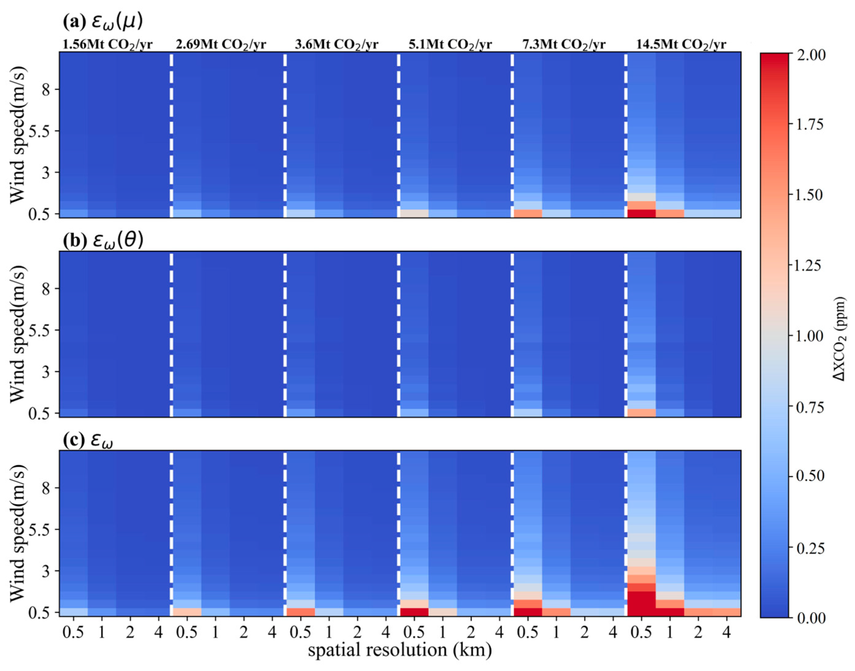
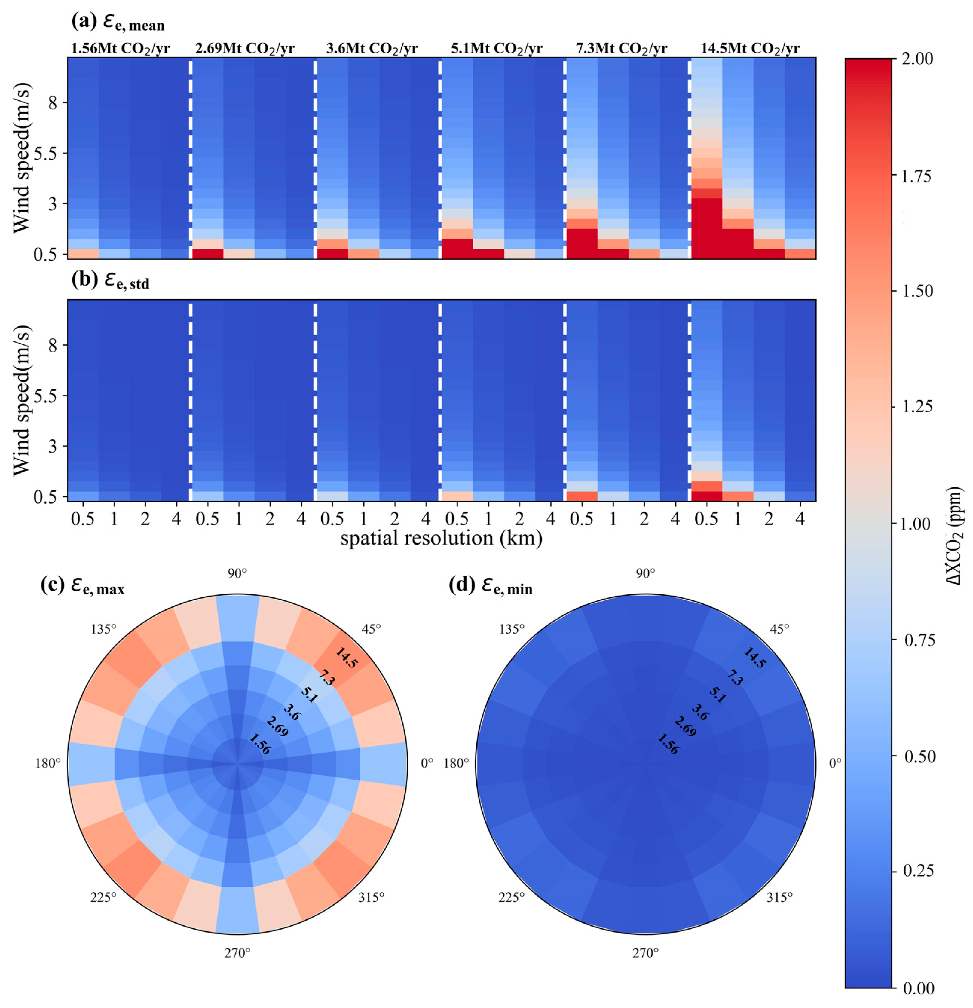
Our results indicate that ε_w(μ) plays a dominant role in the variation of simulated XCO₂ uncertainty introduced by uncertainties in both wind speed and wind direction. With the assumption of a 10% uncertainty in both wind speed and wind direction, for a small-sized power plant (5.1 Mt CO₂/yr) under conditions of wind speed increasing from 0.5 m/s to 4 m/s, the ε_w reduces from 3.75 ± 2.01 ppm to 0.46 ± 0.24 ppm for 1 × 1 km² pixel size, while it changes from 1.82 ± 0.95 ppm to 0.22 ± 0.11 ppm for 1 × 1 km². These variations highlight the sensitivity of satellite detection capabilities to meteorological conditions.

(4)

The overall uncertainty in satellite-detected XCO₂ enhancement was calculated using a combination of uncertainties in wind field, satellite-derived XCO₂ error, and CO₂ emission levels, considering various ε_s levels (0.5, 0.7, 1.0, and 1.5 ppm) and 10% uncertainty for obtained wind field and CO₂ emission data. The results indicate that ε is significantly influenced by the wind field. Although ε for θ = 45° is larger than that for θ = 270° under the same scenario, satellite has a more effective capability for detecting CO₂ emission at θ = 45° due to a more rapid growth of ΔXCO2_max. A designed spatial resolution of satellite better than 1 km is suggested, because the CO₂ emission from small-sized power plants is much more likely be detected when the wind speed is below 3 m/s.

6. Conclusions

In designing satellite payloads, our approach involves forward simulation of plume dispersion at specific spatial resolutions, allowing us to assess whether these results meet the monitoring precision requirements set by the satellite. Once the satellite’s resolution and monitoring precision are confirmed, further refinement of parameters such as signal-to-noise ratio, sampling rate, and spectral resolution will continue. Throughout the simulation process, we strive to incorporate meteorological factors that influence plume dispersion in real-world scenarios. By leveraging scientifically simulated outcomes, this study offers practical insights for refining payload specifications to meet the demands of scientific missions and achieve effective pollution monitoring results.

This research holds significant implications for the design and operation of future CO₂ monitoring satellites, such as the Chinese Tansat2. By focusing on simulating plume dispersion based on satellite spatial resolution and monitoring precision, we explore the satellite’s capability to identify plumes under various conditions. With a monitoring precision of 0.7 ppm, the satellite demonstrates effective capturing of emissions from small to medium-scale ground point sources. Through simulations of point sources with different emission capacities and consideration of wind errors, point source emission rate errors, and satellite monitoring errors, we conduct a quantitative analysis of plume simulation accuracy at different resolutions. Our findings indicate that under typical wind speed conditions, a satellite spatial resolution of 1 km enables effective monitoring of ground point source emissions.

The quantitative analysis of uncertainties and detection capabilities across different scenarios serves as a foundation for future advancements in satellite monitoring of anthropogenic CO₂ emissions, essential for addressing challenges related to climate change. Subsequent work could focus on refining these simulations with actual satellite data and extending the analysis using complex models to simulate more realistic CO₂ plumes.

References

1. Intergovernmental Panel on Climate Change (IPCC). Summary for Policymakers. In Climate Change 2021—The Physical Science Basis: Working Group I Contribution to the Sixth Assessment Report of the Intergovernmental Panel on Climate Change; Climate Change 2021—The Physical Science Basis; Cambridge University Press: Cambridge, UK, 2023; pp. 3–32. [Google Scholar] [CrossRef]
2. UNFCCC. UNFCCC (United Nation Framework Convention on ClimateChange): Decision 18/CMA.1 Modalities, Procedures Andguidelines for the Transparency Framework for Action Andsupport Referred to in Article 13 of the Paris Agreement, FCCC/PA/CMA/2018/Add.2. 2018. Available online: https://unfccc.int/sites/default/files/resource/cma2018_3_add2_new_advance.pdf (accessed on 19 July 2020).
3. Janssens-Maenhout, G.; Pinty, B.; Dowell, M.; Zunker, H.; Andersson, E.; Balsamo, G.; Bézy, J.L.; Brunhes, T.; Bösch, H.; Bojkov, B.; et al. Toward an Operational Anthropogenic CO2 Emissions Monitoring and Verification Support Capacity. Bull. Am. Meteorol. Soc. 2020, 101, E1439–E1451. [Google Scholar] [CrossRef]
4. Ritchie, H.; Rosado, P.; Roser, M. CO2 and Greenhouse Gas Emissions. Our World Data. 2020. Available online: https://ourworldindata.org/co2-and-greenhouse-gas-emissions (accessed on 1 January 2024).
5. Taylor, T.E.; Eldering, A.; Merrelli, A.; Kiel, M.; Somkuti, P.; Cheng, C.; Rosenberg, R.; Fisher, B.; Crisp, D.; Basilio, R.; et al. OCO-3 early mission operations and initial (vEarly) XCO2 and SIF retrievals. Remote Sens. Environ. 2020, 251, 112032. [Google Scholar] [CrossRef]
6. Hakkarainen, J.; Szeląg, M.E.; Ialongo, I.; Retscher, C.; Oda, T.; Crisp, D. Analyzing nitrogen oxides to carbon dioxide emission ratios from space: A case study of Matimba Power Station in South Africa. Atmos. Environ. X 2021, 10, 100110. [Google Scholar] [CrossRef]
7. Kuhlmann, G.; Henne, S.; Meijer, Y.; Brunner, D. Quantifying CO2 Emissions of Power Plants with CO2 and NO2 Imaging Satellites. Front. Remote Sens. 2021, 2, 689838. [Google Scholar] [CrossRef]
8. Liu, L.Y.; Chen, L.F.; Liu, Y.; Yang, D.X.; Zhang, X.Y.; Lu, N.M.; Ju, W.M.; Jiang, F.; Yin, Z.S.; Liu, G.H.; et al. Satellite remote sensing for global stocktaking: Methods, progress and perspectives. Natl. Remote Sens. Bull. 2022, 26, 243–267. [Google Scholar] [CrossRef]
9. He, Z.; Lei, L.; Zeng, Z.-C.; Sheng, M.; Welp, L.R. Evidence of Carbon Uptake Associated with Vegetation Greening Trends in Eastern China. Remote Sens. 2020, 12, 718. [Google Scholar] [CrossRef]
10. Sheng, M.; Lei, L.; Zeng, Z.-C.; Rao, W.; Song, H.; Wu, C. Global land 1° mapping dataset of XCO2 from satellite observations of GOSAT and OCO-2 from 2009 to 2020. Big Earth Data 2022, 7, 170–190. [Google Scholar] [CrossRef]
11. Oda, T.; Feng, L.; Palmer, P.I.; Baker, D.F.; Ott, L.E. Assumptions about prior fossil fuel inventories impact our ability to estimate posterior net CO2 fluxes that are needed for verifying national inventories. Environ. Res. Lett. 2023, 18, 124030. [Google Scholar] [CrossRef]
12. Yao, L.; Liu, Y.; Yang, D.; Cai, Z.; Wang, J.; Lin, C.; Lu, N.; Lyu, D.; Tian, L.; Wang, M.; et al. Retrieval of solar-induced chlorophyll fluorescence (SIF) from satellite measurements: Comparison of SIF between TanSat and OCO-2. Atmos. Meas. Tech. 2022, 15, 2125–2137. [Google Scholar] [CrossRef]
13. Mousavi, S.M.; Dinan, N.M.; Ansarifard, S.; Sonnentag, O. Analyzing spatio-temporal patterns in atmospheric carbon dioxide concentration across Iran from 2003 to 2020. Atmos. Environ. X 2022, 14, 100163. [Google Scholar] [CrossRef]
14. Zheng, B.; Chevallier, F.; Ciais, P.; Broquet, G.; Wang, Y.; Lian, J.; Zhao, Y. Observing carbon dioxide emissions over China’s cities and industrial areas with the Orbiting Carbon Observatory-2. Atmos. Chem. Phys. 2020, 20, 8501–8510. [Google Scholar] [CrossRef]
15. Hill, T.; Nassar, R. Pixel Size and Revisit Rate Requirements for Monitoring Power Plant CO2 Emissions from Space. Remote Sens. 2019, 11, 1608. [Google Scholar] [CrossRef]
16. Reuter, M.; Buchwitz, M.; Schneising, O.; Krautwurst, S.; O’Dell, C.W.; Richter, A.; Bovensmann, H.; Burrows, J.P. Towards monitoring localized CO2 emissions from space: Co-located regional CO2 and NO2; enhancements observed by the OCO-2 and S5P satellites. Atmos. Chem. Phys. 2019, 19, 9371–9383. [Google Scholar] [CrossRef]
17. Kiel, M.; Eldering, A.; Roten, D.D.; Lin, J.C.; Feng, S.; Lei, R.; Lauvaux, T.; Oda, T.; Roehl, C.M.; Blavier, J.-F.; et al. Urban-focused satellite CO2 observations from the Orbiting Carbon Observatory-3: A first look at the Los Angeles megacity. Remote Sens. Environ. 2021, 258, 112314. [Google Scholar] [CrossRef]
18. Liu, J.; Bowman, K.W.; Schimel, D.S.; Parazoo, N.C.; Jiang, Z.; Lee, M.; Bloom, A.A.; Wunch, D.; Frankenberg, C.; Sun, Y.; et al. Contrasting carbon cycle responses of the tropical continents to the 2015–2016 El Nino. Science 2017, 358, eaam5690. [Google Scholar] [CrossRef] [PubMed]
19. Palmer, P.I.; Feng, L.; Baker, D.; Chevallier, F.; Bosch, H.; Somkuti, P. Net carbon emissions from African biosphere dominate pan-tropical atmospheric CO2 signal. Nat. Commun. 2019, 10, 3344. [Google Scholar] [CrossRef] [PubMed]
20. Eldering, A.; Taylor, T.E.; O’Dell, C.W.; Pavlick, R. The OCO-3 mission: Measurement objectives and expected performance based on 1 year of simulated data. Atmos. Meas. Tech. 2019, 12, 2341–2370. [Google Scholar] [CrossRef]
21. Mousavi, S.M.; Dinan, N.M.; Ansarifard, S.; Borhani, F.; Ezimand, K.; Naghibi, A. Examining the Role of the Main Terrestrial Factors Won the Seasonal Distribution of Atmospheric Carbon Dioxide Concentration over Iran. J. Indian Soc. Remote Sens. 2023, 51, 865–875. [Google Scholar] [CrossRef]
22. Falahatkar, S.; Mousavi, S.M.; Farajzadeh, M. Spatial and temporal distribution of carbon dioxide gas using GOSAT data over IRAN. Environ. Monit. Assess. 2017, 189, 627. [Google Scholar] [CrossRef]
23. Golkar, F.; Mousavi, S.M. Variation of XCO2 anomaly patterns in the Middle East from OCO-2 satellite data. Int. J. Digit. Earth 2022, 15, 1219–1235. [Google Scholar] [CrossRef]
24. Shim, C.; Han, J.; Henze, D.K.; Yoon, T. Identifying local anthropogenic CO2 emissions with satellite retrievals: A case study in South Korea. Int. J. Remote Sens. 2018, 40, 1011–1029. [Google Scholar] [CrossRef]
25. Sierk, B.; Fernandez, V.; Bézy, J.L.; Meijer, Y.; Durand, Y.; Bazalgette Courrèges-Lacoste, G.; Pachot, C.; Löscher, A.; Nett, H.; Minoglou, K.; et al. The Copernicus CO2M mission for monitoring anthropogenic carbon dioxide emissions from space. In Proceedings of the International Conference on Space Optics—ICSO 2020, Online, 30 March–2 April 2021. [Google Scholar]
26. Lin, X.; van der A, R.; de Laat, J.; Eskes, H.; Chevallier, F.; Ciais, P.; Deng, Z.; Geng, Y.; Song, X.; Ni, X.; et al. Monitoring and quantifying CO2 emissions of isolated power plants from space. Atmos. Chem. Phys. 2023, 23, 6599–6611. [Google Scholar] [CrossRef]
27. Sutton, O.G. A theory of eddy diffusion in the atmosphere. Proc. R. Soc. Lond. Ser. A 1932, 135, 143–165. [Google Scholar]
28. Bovensmann, H.; Buchwitz, M.; Burrows, J.P.; Reuter, M.; Krings, T.; Gerilowski, K.; Schneising, O.; Heymann, J.; Tretner, A.; Erzinger, J. A remote sensing technique for global monitoring of power plant CO2 emissions from space and related applications. Atmos. Meas. Tech. 2010, 3, 781–811. [Google Scholar] [CrossRef]
29. Pasquill, F. The estimation of the dispersion of windborne material. Meteorol. Mag. 1961, 90, 33–49. [Google Scholar]
30. Gan, L.; Lu, T.; Shu, Y. Diffusion and Superposition of Ship Exhaust Gas in Port Area Based on Gaussian Puff Model: A Case Study on Shenzhen Port. J. Mar. Sci. Eng. 2023, 11, 330. [Google Scholar] [CrossRef]
31. Hu, Y.; Shi, Y. Estimating CO2 Emissions from Large Scale Coal-Fired Power Plants Using OCO-2 Observations and Emission Inventories. Atmosphere 2021, 12, 811. [Google Scholar] [CrossRef]
32. Tong, D.; Zhang, Q.; Davis, S.J.; Liu, F.; Zheng, B.; Geng, G.; Xue, T.; Li, M.; Hong, C.; Lu, Z.; et al. Targeted emission reductions from global super-polluting power plant units. Nat. Sustain. 2018, 1, 59–68. [Google Scholar] [CrossRef]
33. Pinty, B.; Janssens-Maenhout, G.; Dowell, M.; Zunker, H.; Brunhes, T.; Ciais, P.; Dee, D.; Denier Van Der Gon, H.; Dolman, H.; Drinkwater, M.; et al. An Operational Anthropogenic CO2 Emissions Monitoring & Verification System: Baseline Requirements, Model Components and Functional Architecture; Publications Office of the European Union: Luxembourg, 2021. [Google Scholar]
34. Nassar, R.; Hill, T.G.; McLinden, C.A.; Wunch, D.; Jones, D.B.A.; Crisp, D. Quantifying CO2 Emissions From Individual Power Plants From Space. Geophys. Res. Lett. 2017, 44, 10045–10053. [Google Scholar] [CrossRef]
35. Peischl, J.; Ryerson, T.B.; Holloway, J.S.; Parrish, D.D.; Trainer, M.; Frost, G.J.; Aikin, K.C.; Brown, S.S.; Dubé, W.P.; Stark, H.; et al. A top-down analysis of emissions from selected Texas power plants during TexAQS 2000 and 2006. J. Geophys. Res. Atmos. 2010, 115, D16303. [Google Scholar] [CrossRef]
36. Angevine, W.M.; Peischl, J.; Crawford, A.; Loughner, C.P.; Pollack, I.B.; Thompson, C.R. Errors in top-down estimates of emissions using a known source. Atmos. Chem. Phys. 2020, 20, 11855–11868. [Google Scholar] [CrossRef]
Figure 1. Statistics of power plant number (a,b) and cumulative emission (c,d) in 2019 from GPED v1.1. Left column is for power plants in China, and right column is for global data.
Sensors 24 01881 g001
Figure 2. Plume simulations of XCO2 observations relative to a constant 420 ppm background for satellite-based XCO2 error of 0.7 ppm (a) and 1.5 ppm (b). Column 1 shows the simulated Gaussian plume at 50 m resolution for each power plant emission rate against a clean background. Columns 2~5 are simulated observations with a spatial resolution of 0.5, 1, 2 and 4 km, respectively. Top to bottom rows in each panel are simulated observations for CO2 emission of 6, 13, and 25 Mt CO2/yr, respectively.
Sensors 24 01881 g002
Figure 3. XCO2 enhancement distribution and ΔXCO2max simulations with μ = 4 m/s and θ = 270°. Column 1 shows the simulated Gaussian plume at 50 m resolution for each power plant emission rate against a clean background. Columns 2~5 are simulated observations with a spatial resolution of 0.5, 1, 2 and 4 km, respectively. Top to bottom rows are simulated observations for CO2 emissions of 0.184, 1.56, 2.69, 3.6, 5.1, 7.3 and 14.5 Mt CO2/yr, respectively.
Sensors 24 01881 g003
Figure 4. XCO2 enhancement distribution and ΔXCO2max simulations with μ = 2 m/s and θ = 270°. Column 1 shows the simulated Gaussian plume at 50 m resolution for each power plant emission rate against a clean background. Columns 2~5 are simulated observations with a spatial resolution of 0.5, 1, 2 and 4 km, respectively. Top to bottom rows are simulated observations for CO2 emissions of 0.184, 1.56, 2.69, 3.6, 5.1, 7.3 and 14.5 Mt CO2/yr, respectively.
Sensors 24 01881 g004
Figure 5. XCO2 enhancement distribution and ΔXCO2max simulations with μ = 4 m/s and θ = 45°. Column 1 shows the simulated Gaussian plume at 50 m resolution for each power plant emission rate against a clean background. Columns 2~5 are simulated observations with a spatial resolution of 0.5, 1, 2 and 4 km, respectively. Top to bottom rows are simulated observations for CO2 emissions of 0.184, 1.56, 2.69, 3.6, 5.1, 7.3 and 14.5 Mt CO2/yr, respectively.
Sensors 24 01881 g005
Figure 6. Box plots and line charts of the ΔXCO2max simulation results for θ = 270° and μ from 0.5 to 10 m/s. (af) are corresponding to emissions of 1.56, 2.69, 3.6, 5.1, 7.3 and 14.5 Mt CO2/yr, the green dotted and orange lines represent the mean and median, respectively.
Sensors 24 01881 g006
Figure 7. Means (a) and standard deviations (b) of ΔXCO2max for fixed θ and different μ values (0.5~10 m/s) in polar coordinates.
Sensors 24 01881 g007
Figure 8. ΔXCO2max means with fixed μ and different θ values (0°~360°) for different spatial resolutions of satellite. Error bars show the standard deviations of ΔXCO2max in the binned μ. (af) are corresponding to emissions of 1.56, 2.69, 3.6, 5.1, 7.3 and 14.5 Mt CO2/yr, respectively.
Sensors 24 01881 g008
Figure 9. The simulated uncertainties of ΔXCO2 associated with the wind field for θ = 45°. (a), (b) and (c) are for εw(μ), εw(θ) and εw, respectively.
Sensors 24 01881 g009
Figure 10. The simulated uncertainties of ΔXCO2 associated with the wind field for θ = 270°. (a), (b) and (c) are for εw(μ), εw(θ) and εw, respectively.
Sensors 24 01881 g010
Figure 11. Statistical results of the simulated uncertainties in ΔXCO2 associated with the wind field. (a) and (b) are for means and standard deviations of εw values at different wind speeds, respectively. (c) and (d) are for maximums and minimums of εw at different wind directions, respectively.
Sensors 24 01881 g011
Figure 12. Statistical results of the simulated uncertainties in ΔXCO2 associated with the wind field. (a) and (b) are for means and standard deviations of εe values at different wind speeds, respectively. (c) and (d) are for maximums and minimums of εe at different wind directions, respectively.
Sensors 24 01881 g012
Figure 13. Overall uncertainties in satellite-detected XCO2 enhancement and the difference between them and ΔXCO2max for θ = 45°. (ad) are ε values calculated from εs = 0.5, 0.7, 1.0 and 1.5 ppm, respectively. (eh) are results of ΔXCO2max subtracted from ε for εs = 0.5, 0.7, 1.0 and 1.5 ppm, respectively.
Sensors 24 01881 g013
Figure 14. Overall uncertainties in satellite-detected XCO2 enhancement and the difference between them and ΔXCO2max for θ = 270°. (ad) are ε values calculated from εs = 0.5, 0.7, 1.0 and 1.5 ppm, respectively. (eh) are results of ΔXCO2max subtracted from ε for εs = 0.5, 0.7, 1.0 and 1.5 ppm, respectively.
Sensors 24 01881 g014
Disclaimer/Publisher’s Note: The statements, opinions and data contained in all publications are solely those of the individual author(s) and contributor(s) and not of MDPI and/or the editor(s). MDPI and/or the editor(s) disclaim responsibility for any injury to people or property resulting from any ideas, methods, instructions or products referred to in the content.