Abstract
In this article, the issue of joint state and fault estimation is ironed out for delayed state-saturated systems subject to energy harvesting sensors. Under the effect of energy harvesting, the sensors can harvest energy from the external environment and consume an amount of energy when transmitting measurements to the estimator. The occurrence probability of measurement loss is computed at each instant according to the probability distribution of the energy harvesting mechanism. The main objective of the addressed problem is to construct a joint state and fault estimator where the estimation error covariance is ensured in some certain sense and the estimator gain is determined to accommodate energy harvesting sensors, state saturation, as well as time delays. By virtue of a set of matrix difference equations, the derived upper bound is minimized by parameterizing the estimator gain. In addition, the performance evaluation of the designed joint estimator is conducted by analyzing the boundedness of the estimation error in the mean-squared sense. Finally, two experimental examples are employed to illustrate the feasibility of the proposed estimation scheme.
1. Introduction
In recent years, state estimation has gained unprecedented enthusiasm due to the swift advancement of information technology and signal processing, notably in automatic control systems, target tracking, and navigation positioning [1,2,3]. Ongoing research strives for more precise, robust, and computationally efficient state estimation methods to address the evolving demands of applications. Generally, the existing algorithms have been categorized by diverse performance criteria, including Kalman filtering and its variants, estimation scheme, and recursive state estimation. Specifically, the well-known Kalman filtering performs as a global optimal estimation scheme with the assumption of the statistical characteristics of the system noise being known accurately, while filtering relies on the infinite norm of the output-to-interference signal ratio. It should be pointed out that both the above-mentioned estimation schemes exhibit significant deviation when it comes to the nonlinearities/uncertainties. As a suboptimal Kalman-type estimation scheme, recursive state estimation is applied to accommodate the nonlinearities/uncertainties in the sense of the upper bound on estimation error covariances being minimized [4,5,6].
In existing state estimation algorithms, sensors are often assumed to operate without faults. Unfortunately, in engineering practice, various destabilizing factors emerge, including unknown external disturbances, unpredictable fluctuations in parameters, and alterations in system structure [7,8,9]. Such factors give rise to randomly occurring faults, resulting in performance degradation and/or extreme system instability. Especially in sensor networks, such faults are unmeasurable. It is essential to incorporate fault estimation, utilizing known information to estimate fault signals. To date, considerable research has been dedicated to exploring fault estimation [10,11,12,13]. For example, in [11], the issue of distributed fault-tolerant state estimation in stochastic systems across sensor networks affected by intermittent faults was explored. In [13], the investigation delved into a novel hybrid observer-based fault estimation scheme within cyber–physical systems for the joint estimation of state and faults. However, the majority of current research does not account for the impact of random faults on the results of state estimation, which constitutes one of the motivations of this article.
It is well known that measurement is one of the most crucial parts of the issue of state estimation. The conventional battery-powered approach relies on wireless sensor networks and is actually facing a series of limitations, especially the limited battery capacity [14,15]. For the sake of avoiding the energy depletion of communication devices, the so-called energy harvesting technology is invented which has the prominent feature of capturing the scattered energy resources from the external environment, encompassing solar energy, wind energy, mechanical vibration, etc. [16,17]. Then the harvested energy is converted into internally stored energy, replacing the traditional sensor power supply methods. Therefore, the wireless sensor networks achieve sustainable self-sufficiency and liberation from the limitations of sensor battery lifespans [18,19]. Nevertheless, energy harvesting sensors still bring some new challenges. Different from sensors powered by conventional batteries, a significant aspect lies in that the energy collected by the energy harvesting sensors is actually random and intermittent [20,21]. This characteristic primarily arises from the stochastic nature of the energy harvested from the external environment.
Hence, in the widespread usage of energy-harvesting sensors, ensuring continuous adequacy of stored energy at all times becomes a formidable challenge. Insufficient energy levels in sensors can lead to inevitable communication interruptions between adjacent nodes, consequently causing missing measurements. Currently, regarding the mentioned issues, energy harvesting technology has sparked a series of research interests; see, e.g., [22,23,24,25]. For instance, in [24], researchers addressed energy-dependent remote state estimation in nonlinear time-delayed systems, employing a recursive calculation for the energy level probability distribution. In [25], the state and fault estimation problem for time-varying systems with energy harvesting sensors has been investigated. In addition, inherent physical constraints in practical applications contribute to the prevalent occurrence of inevitable state saturation. Generally, state saturation is essentially the specific nonlinearity that constrains state variables in a certain boundary, which may lead to a degradation in the performance of state estimation algorithms [26,27,28]. Therefore, it is crucial to account for this phenomenon when tackling filtering/state estimation challenges. In the past decade, a substantial number of solutions and strategies have arisen for specific state estimation problems with state saturation; see, e.g., [29,30,31,32]. For example, in [30], the joint estimation problem with saturation and nonlinearity was studied, where the system was reorganized into a singular system and an estimator was designed at each node for effective estimation. In [32], a recursive filter was designed against state saturations and probabilistic attacks in an array of two-dimensional shift-varying systems.
To the best of the author’s knowledge, there has not been sufficient research on the joint estimation of state and fault with the system equipped with energy harvesting sensors, not to mention addressing the time-delayed system involving state saturation, nonlinearity, and parameter uncertainty. It is worth mentioning that most current research cannot provide performance analysis of estimation algorithms in such a complex time-delayed system. Meanwhile, existing state estimation algorithms have not fully considered the complex situations in engineering applications, making it difficult to ensure the stability of algorithm performance. As such, the main purpose of this article is to narrow such a gap by comprehensively and deeply researching a novel joint estimation scheme and establishing a sufficient condition to complete the performance analysis of the proposed algorithm. Motivated by the discussions above, the article is dedicated to investigating a joint state and fault estimation scheme for a state-saturated system subject to energy harvesting sensors. The main contributions of the article are outlined as follows:
- The joint state and fault estimation scheme is, for the first time, comprehensively and deeply studied for delayed nonlinear systems with energy harvesting sensors and state saturation;
- A set of matrix difference equations are firstly resorted to recursively compute the upper bound on the estimation error covariance (EEC) and the desired estimator gain is obtained by minimizing the trace of the upper bound on EEC;
- A new approach is invented to compensate for the performance degradation of the estimator caused by random faults, measurement loss due to insufficient energy level as well as sensor saturation;
- The mean-squared exponential boundedness of the estimation error in such a complex engineering context is first analyzed by establishing a sufficient condition.
Finally, two experimental examples are exploited to validate the feasibility of the proposed estimation algorithm.
Notation: The notations used in this article are standard except where otherwise stated. and are the transposition and the inverse of A, respectively. For symmetric matrices U and V, (respectively, ), means that is a positive semi-defined (positive definite) matrix. stands for the mathematical expectation of the stochastic variable . means the trace of the matrix M. represents the occurrence probability of event “”.
2. Problem Formulation
The joint state and fault estimation configuration for a state-saturated system with energy harvesting sensors is shown in Figure 1, where the obtained signals are first processed through a saturation function and the sensors harvest energy for storage. The current energy level of the sensor determines whether the measurement can be transmitted. Meanwhile, the workflow of the joint estimation scheme proposed in this article can be seen in Figure 2. The system under consideration with measurements is given as follows:
where and are, respectively, the state and measurement output at time instant s. and are zero-mean Gaussian white-noise sequences with covariances and . represents the constant delay. , , and are known matrices with compact dimensions. In addition, and are parameter uncertainties with the following relationship
where , and are known time-varying matrices, and denotes the parameter uncertainty satisfying .
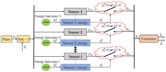
Figure 1.
The joint state and fault estimation configuration for state-saturated system with energy harvesting sensors.

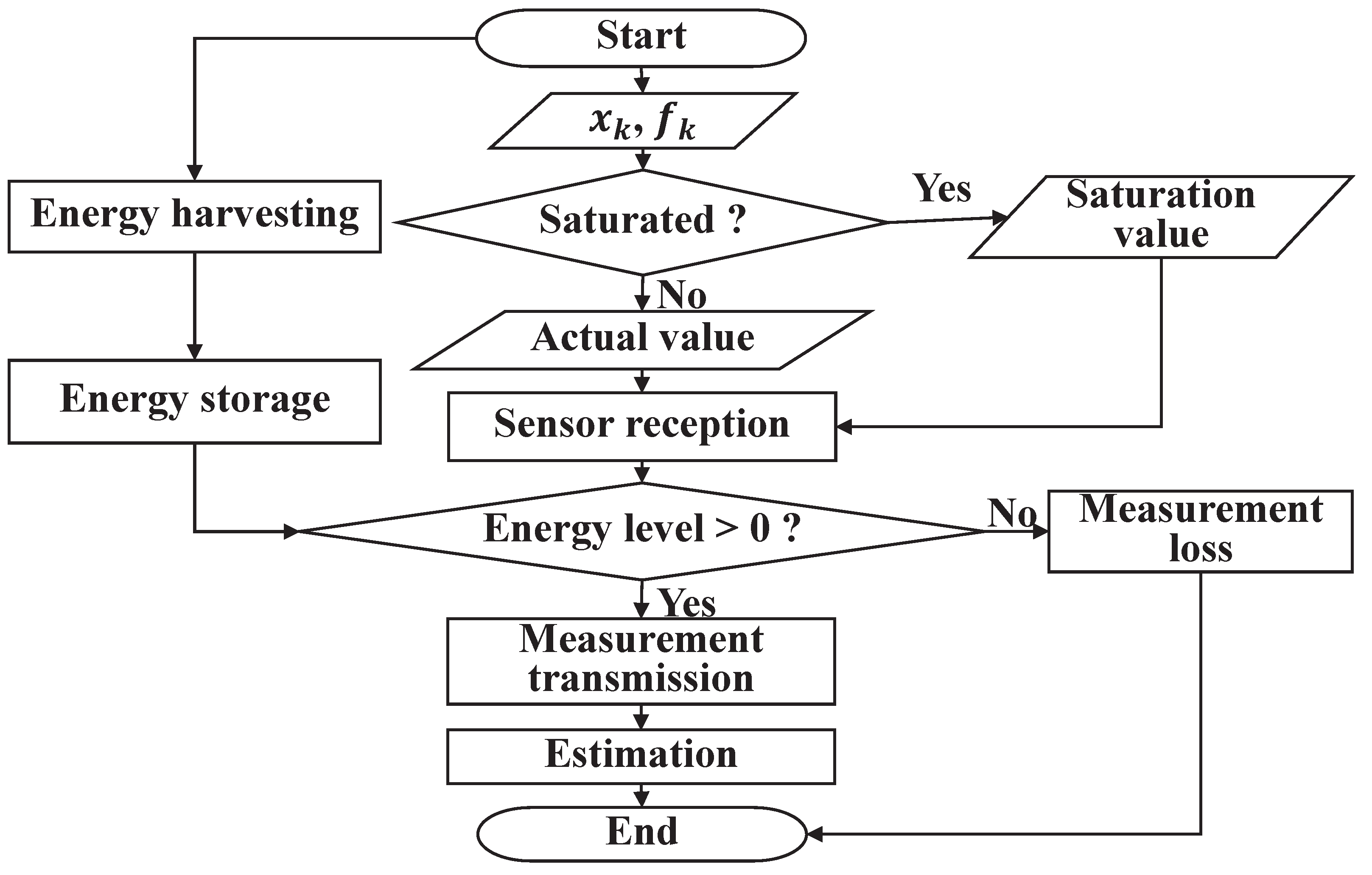
Figure 2.
The workflow diagram of the joint state and fault estimation scheme.
The known nonlinear function satisfies
for all and a known scalar.
The saturation function : ↦ is defined by
with = , where and stand for the ith element of q and saturation level. In addition, denotes the signum function.
The dynamic characteristics of the fault is modeled by
where is a known matrix with appropriate dimension.
The variable is used to characterize the random nature of the fault, which satisfies the following Bernoulli distribution
where is a known scalar.
Remark 1.
The purpose of this article is to design a joint estimation scheme for state and fault, which estimates randomly occurring faults while completing state estimation. The fault involved in this article is a sudden and random fault, which is very common in industrial processes. Its dynamic model is represented by Equation (5). When a fault signal occurs, it will be detected by the system in a timely manner, and then the fault estimation scheme will be used to estimate it. Due to the complexity of the scenarios considered in this article, accurate estimation of fault signals can improve the performance of state estimation.
Assumption A1.
The initial values with the mean and covariance are mutually uncorrelated with , , and .
At each instant s, the energy level of the sensor i is denoted by , where represents the maximum storage capacity of sensor i. The energy harvested by the ith sensor at s is denoted by , which follows an independent identically distributed random process:
with , where and .
When the energy harvesting sensor stores non-zero energy units, it can transmit the measurement to a remote estimator and consumes one unit of energy. Hence, the dynamics of the energy level of the sensor is denoted by
and the measurement transmitted to the remote joint estimator can be written by
where is an indicator variable. where can be given as
Remark 2.
The energy harvesting sensor can be understood as a rechargeable battery that can self charge, and it can harvest, convert, and store energy through the energy harvesting mechanism. When it is necessary to transmit measurement values to a remote estimator, the sensor will evaluate its own energy level. If the energy level meets the consumption demand, the measurement transmission is completed. Otherwise, the measurement loss will emerge. Although energy harvesting sensors also have the risk of measurement loss, their loss rate is far lower than traditional power supply methods, and the impact in industrial processes is minimal.
Setting . Based on Equation (1), we have the following augmented system:
where
Based on the received measurements , we construct the joint estimator as follows.
where and represent the one-step prediction and the estimation of at s, respectively. is the estimator gain to be designed, and .
Letting the prediction error be and the estimation error be , the following error dynamics are obtained from Equations (11) and (13):
The main purpose of this article is to design a joint state and fault estimator of the form Equation (13) for the considered state-saturated system Equation (1) equipped with energy harvesting sensors such that for all energy-harvesting-induced measurements and state saturations, the upper bound on EEC is guaranteed and minimized by the estimator gain . Furthermore, a sufficient condition is given to evaluate the boundedness analysis of the estimation error in a mean-squared sense.
3. Joint State and Fault Estimation
This section provides an upper bound on EEC through mathematical induction, and then such upper bound is minimized by a set of matrix difference equations. Furthermore, a sufficient criterion has been formulated to verify the exponential boundedness of the estimation error in a mean-squared sense. The following lemmas will facilitate further development of the article.
Lemma 1.
Suppose that and are given scalars, there exists a constant matrix such that
where stands for the saturation function in Equation (4).
Proof.
When , we can have that and then we can get . When , we can get that and then we can choose any real number . Similarly, when , it is easy to complete the proof. □
Lemma 2.
Given any vectors and , the following inequality holds
where is an arbitrary scalar.
Proof.
The proof can refer to [33], omitted here. □
Lemma 3.
The measurement of transmission probability at s is derived as
Proof.
The probability distribution of the energy level can be written by
Based on Equation (8), the energy is independent of . Hence, for , we have:
Then, the probability can be expressed by
Here, for the energy level in Equation (8), the recursion of the probability distribution can be computed by
where and
According to Equation (10), one immediately has
which ends the proof. □
With the help of Lemma 1, Equation (14) can be rewritten as
where with .
By noting and , the prediction error covariance and EEC are, respectively, given by
and
Theorem 1.
then is an upper bound on , i.e., .
Let the positive scalars be given. The prediction error covariance and EEC are given in Equations (16) and (17), respectively. If the matrices satisfy the following equations
and
with , where
Proof.
The proof of Theorem 1 is given in Appendix A. □
In the following theorem, the joint estimator gain has been design to minimize the upper bound in Theorem 1.
Theorem 2.
The trace of the upper bound on EEC in Theorem 1 is minimized by the following estimator gain
where
Proof.
The trace of the can be computed as follows:
In order to compute the optimal estimator gain , we take the partial derivative of the trace of with respect to
Letting , one has
which ends the proof. □
Remark 3.
Based on the above discussion, we obtained an upper bound on the EEC in Theorem 1, and in Theorem 2, we obtained the estimator gain by minimizing this upper bound. Therefore, we have successfully resolved the issue of the joint state and fault estimation for the state-saturated system equipped with energy harvesting sensors. In addition, to better demonstrate the workflow of our algorithm, a simple flowchart is shown in Figure 2.
In the following theorem, we are poised to assess the effectiveness of the designed estimation scheme and establish a sufficient condition to ensure the exponential boundedness of the estimation error in a mean-squared sense.
Definition 1.
The stochastic process is considered to be exponentially bounded in mean-squared sense if there exist real numbers and such that
holds for any .
Theorem 3.
Suppose that , , , , , , , , , , , , , , , , , , , , , , , , , , , are positive scalars, if the following inequalities
hold, then the estimation error is exponentially bounded in mean-squared sense.
Proof.
The proof of Theorem 3 is given in Appendix B. □
4. Simulation Experiments
In this section, we intend to provide two experimental examples to show the feasibility of the proposed joint state and fault estimation scheme. Moreover, in Example 1, a performance comparison was made between the Kalman filtering and the proposed algorithm.
Example 1.

Consider the delayed state-saturated system Equation (1) equipped with energy harvesting sensors with the following parameters:
The noise and are zero-mean Gaussian noises, respectively, with covariances and . The time delay is set as and the saturation level is set as . Suppose that the initial energy unit stored in the sensor is , meanwhile, the sensor has a maximum storage capacity of energy units. The random variable is chosen as . Based on the above parameters, the estimator parameter can be computed at each instant by recurring to Equation (20). Furthermore, the recursive computation of the probability distribution of the sensor energy level and the expectation of the measurement transmission is presented in Table 1.
Table 1.
Results for energy harvesting sensors.
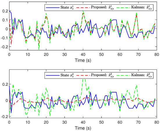
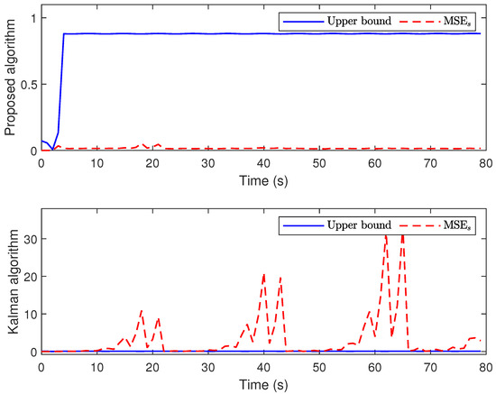
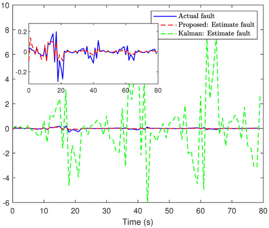
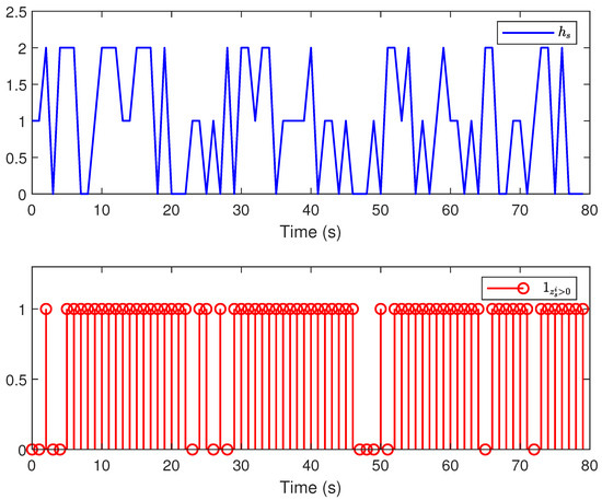
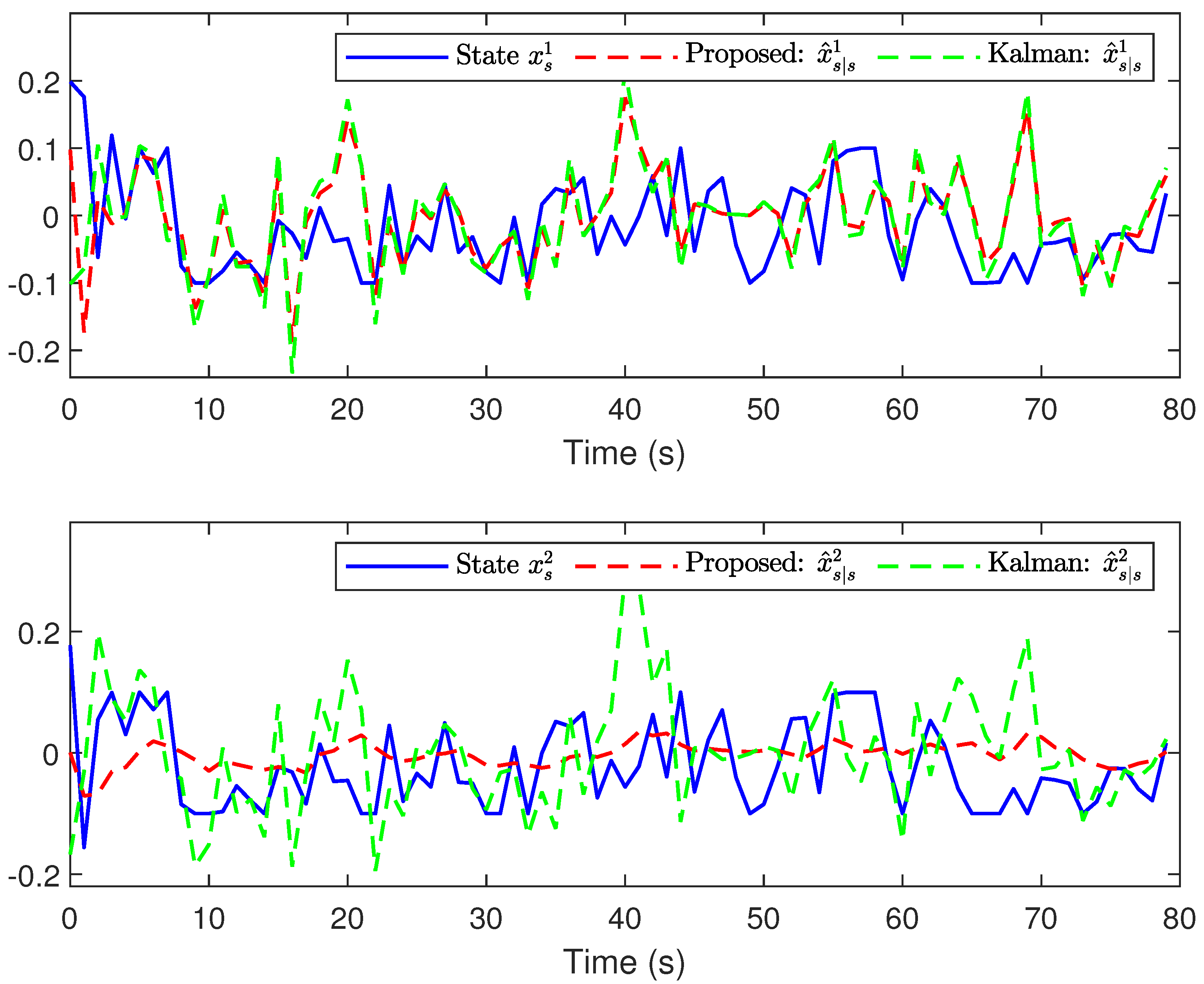
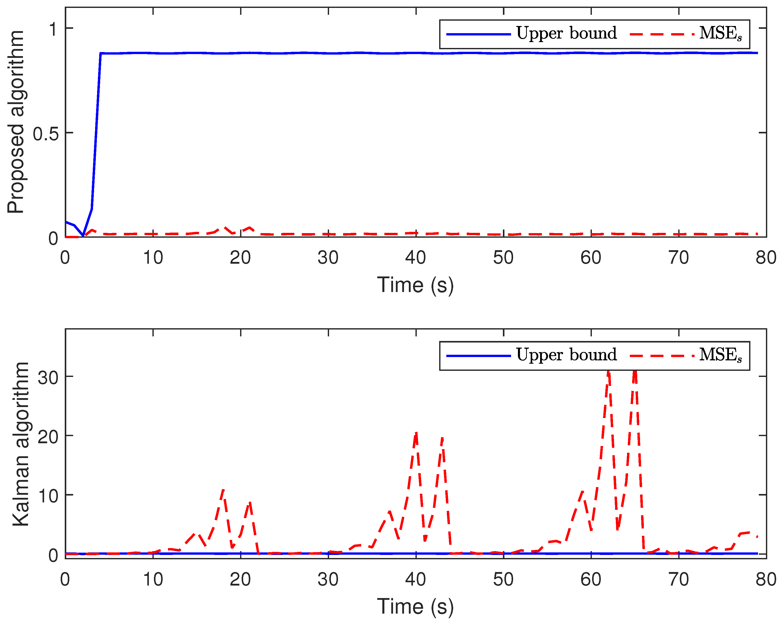
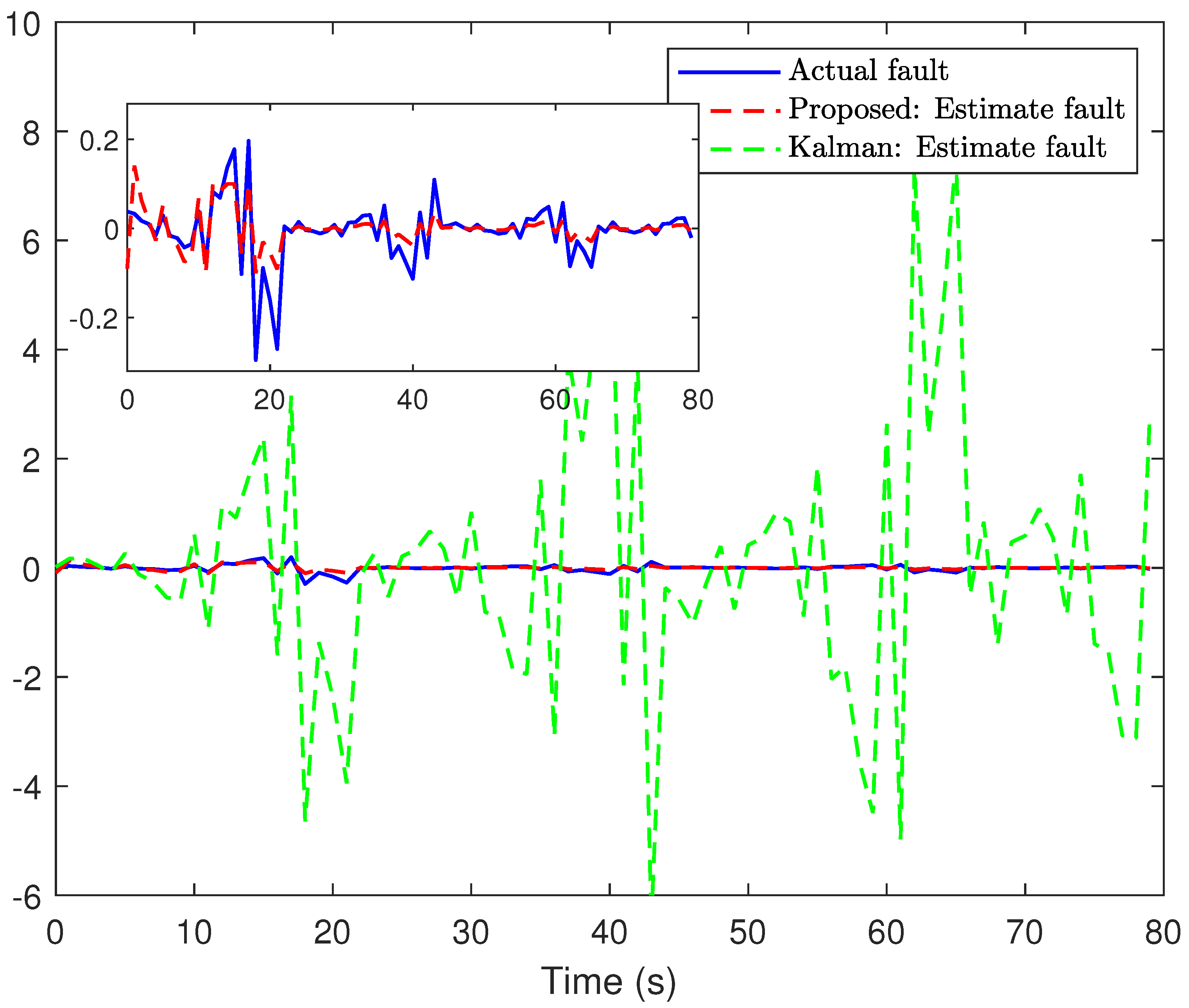
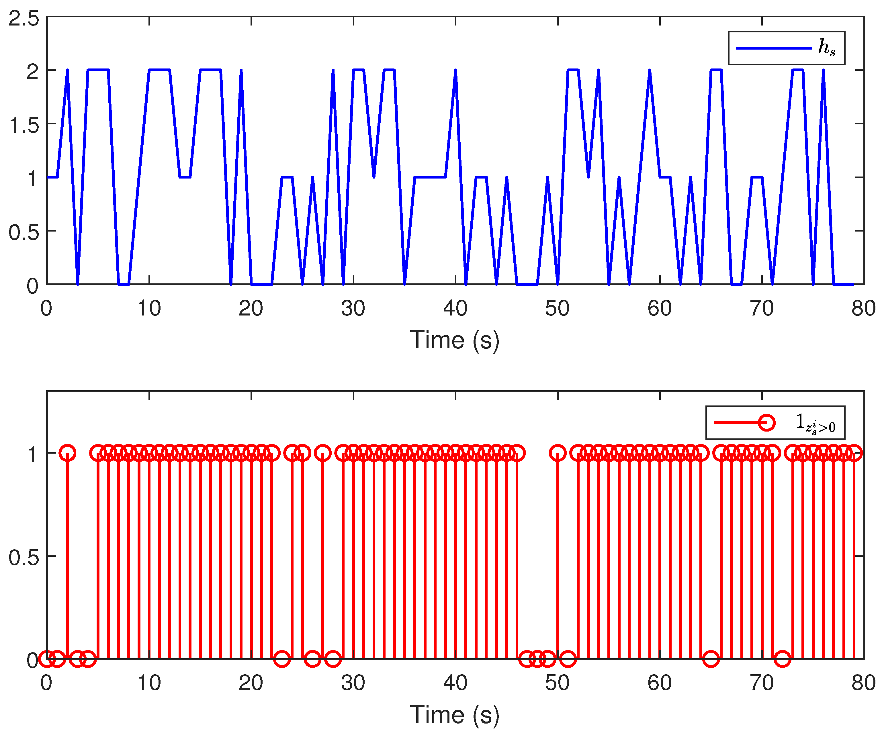
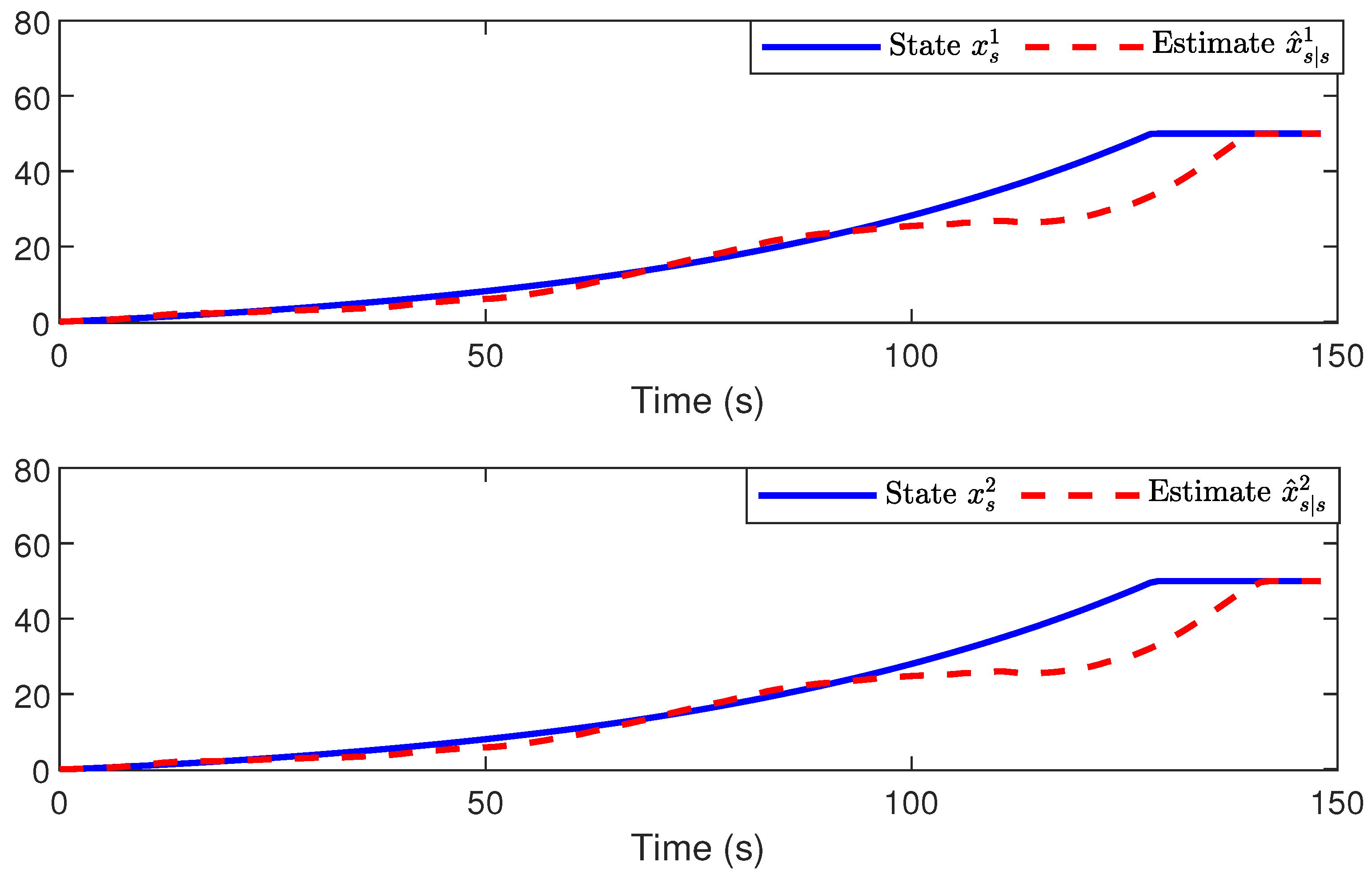
The main results are listed in Figure 3, Figure 4, Figure 5 and Figure 6. Figure 3 plots the actual states and their estimates for and . Figure 5 depicts the trace of the minimum upper bound and the mean square error (MSE) (defined by ) for the estimation of the state variables. The faults and their estimates are depicted in Figure 4. Figure 6 depicts the values of and at each instant. Overall, based on the comparison results between the proposed algorithm and the Kalman filtering algorithm shown in Figure 3, Figure 4 and Figure 5, it is not difficult to find that the proposed algorithm has better estimation performance when facing the complex situations considered in this article.
Figure 3.
State , and their estimates.
Figure 4.
The trace of the upper bounds and estimation error covariances.
Figure 5.
The faults and their estimates.
Figure 6.
The energy harvested and energy consumption at time instant s.
Example 2.
Considering the target tracking task [34] in Equation (1) with the following parameters:
The initial state of the target system is given as . We set and , and we choose the saturation levels as . The sampling period is selected as . Other parameters are the same as Example 1.
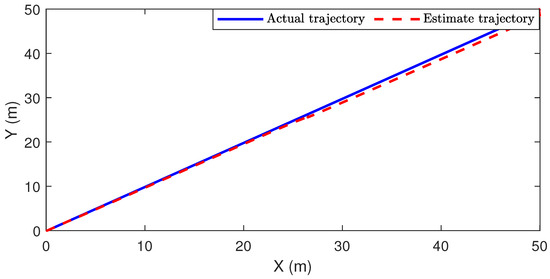
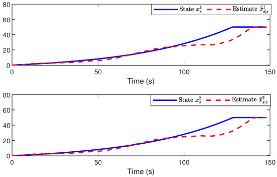
The simulation results are shown in Figure 7 and Figure 8. To be specific, Figure 7 plots the actual moving trajectory and the position estimate of the target in the two-dimensional plane. Moreover, the plotted figures in Figure 8 illustrate both the actual coordinates and of the target position and their corresponding estimates. It is evident that the proposed estimation scheme exhibits satisfactory performance.
Figure 7.
The actual moving trajectory and the position estimate of the target.
Figure 8.
The actual coordinates and of the target position and their estimates.
5. Conclusions
In this article, we have committed to studying a joint state and fault estimation scheme for state-saturated system subject to energy harvesting sensors. The energy-harvesting-induced missing measurements have been considered where the occurrence probability of this phenomenon has been computed at each instant. A joint state and fault estimator has been developed where upper bound on EEC has been ensured and then be minimized by appropriately designing the joint estimator gain. Moreover, the performance of the estimation scheme has been conducted by analyzing the boundedness of the estimation error. Finally, two experimental examples are employed to illustrate the effectiveness of the proposed estimation scheme, and the results show that the designed estimator has excellent estimation performance and performs well in target tracking. With the continuous expansion of application scenarios, state estimation/filtering algorithms are facing increasingly unstable factors, and relevant research should be based on industrial applications to make algorithms adapt to actual demands. In the future, based on the research results of this article, we will devote to the state estimation problems subject to time-correlated fading channels [35] and multiple description coding scheme [36].
Author Contributions
Methodology, Q.S., R.G. and P.P.; Software, L.Z.; Formal analysis, L.Z.; Investigation, C.H. and R.G.; Resources, P.P.; Writing—original draft, L.Z. and P.P.; Writing—review and editing, C.H. and Q.S.; Supervision, C.H. and Q.S. All authors have read and agreed to the published version of the manuscript.
Funding
This work was supported in part by the National Natural Science Foundation of China under Grant 62001254 and 52202496, the 333 Talent Technology Research Project of Jiangsu under Grants 2022021, and the Natural Science Foundation of the Higher Education Institutions of Jiangsu Province under Grants 22KJB510040, the Basic Science Research Program of Nantong City under Grant JC12022028, and the Nantong social livelihood science and technology project under Grant MS12022015.
Institutional Review Board Statement
Not applicable.
Informed Consent Statement
Not applicable.
Data Availability Statement
No new data were created or analyzed in this study. Data sharing is not applicable to this article.
Conflicts of Interest
The authors declare no conflicts of interest.
Appendix A
Proof.
We tend to proof this theorem through mathematical derivation. It is can be seen from the initial condition that . Suppose that , then we only need to show that .
By utilizing Lemma 2, it can be derived from Equation (16) that
Using Lemma 2 again, the term and can be computed as:
and
Furthermore, since the is constrained by the saturation function, which implies
and
Combining Equations (A2)–(A5), one has
and
It follows from Equations (A1), (A6) and (A7) that
Furthermore, it can also be obtained that
Therefore, combining Equations (A8) and (A9), one has
Subsequently, we are in a position to prove that . By virtue of Lemma 2, it can be obtained from Equation (17) that
By noting Lemma 2 and Equation (3), the upper bound of can be derived as follows:
It follows from Equations (19), (A10) and (A11) that . The proof is now complete. □
Appendix B
Proof.
According to Equation (15), we have
where
From Equation (20), we have
Similarly, it is clear from the first term in Equation (A14) that
Next, it follows from Lemma 2 and Equation (24) that
and
Subsequently, contemplate the following iterative matrix equation
where and is a scalar. Then, based on the above iterative matrix equation, we arrive at
where is defined as in Equation (24).
It can be deduced from that
On the other hand, we have
Considering Equations (A21) and (A22), two positive scalars and can be identified such that holds for all .
Set . It follows from Lemma 2 and Equation (A13) that
In light of the matrix inversion lemma and the definition of the matrix , we have
Substituting Equation (A24) into Equation (A23), which implies
with . Then, based on Equation (A25), we have
where . It is not difficult to see that for . Furthermore, we obtain that
In accordance with Definition 1, we conclude that the stochastic process is exponentially bounded in mean-squared sense. □
References
- Duník, J.; Biswas, S.K.; Dempster, A.G.; Pany, T.; Closas, P. State estimation methods in navigation: Overview and application. IEEE Aerosp. Electron. Syst. Mag. 2020, 35, 16–31. [Google Scholar] [CrossRef]
- Liu, Y.; Ji, X.; Yang, K.; He, X.; Na, X.; Liu, Y. Finite-time optimized robust control with adaptive state estimation algorithm for autonomous heavy vehicle. Mech. Syst. Signal Process. 2020, 139, 106616. [Google Scholar] [CrossRef]
- Zhou, L.; Lai, X.; Li, B.; Yao, Y.; Yuan, M.; Weng, J.; Zheng, Y. State estimation models of lithium-ion batteries for battery management system: Status, challenges, and future trends. Batteries 2023, 9, 131. [Google Scholar] [CrossRef]
- Chen, T.; Ren, H.; Foo, E.; Li, P.; Amaratunga, G. An agent-based distributed state estimation approach for interconnected power systems. IEEE Syst. J. 2023, 17, 3016–3025. [Google Scholar] [CrossRef]
- Shen, Y.; Wang, Z.; Dong, H.; Lu, G.; Alsaadi, F.E. Distributed recursive state estimation for a class of multi-rate nonlinear systems over wireless sensor networks under flexray protocols. IEEE Trans. Netw. Sci. Eng. 2023, 10, 1551–1563. [Google Scholar] [CrossRef]
- Shen, B.; Wang, Z.; Wang, D.; Liu, H. Distributed state-saturated recursive filtering over sensor networks under round-robin protocol. IEEE Trans. Cybern. 2020, 50, 3605–3615. [Google Scholar] [CrossRef] [PubMed]
- Dong, H.; Wang, Z.; Ding, S.; Gao, H. Finite-horizon estimation of randomly occurring faults for a class of nonlinear time-varying systems. Automatica 2014, 50, 3182–3189. [Google Scholar] [CrossRef]
- Huang, C.; Coskun, S.; Zhang, X.; Mei, P. State and fault estimation for nonlinear systems subject to censored measurements: A dynamic event-triggered case. Int. J. Robust Nonlinear Control 2022, 32, 4946–4965. [Google Scholar] [CrossRef]
- Huang, C.; Shen, B.; Zou, L.; Shen, Y. Event-triggering state and fault estimation for a class of nonlinear systems subject to sensor saturations. Sensors 2021, 21, 1242. [Google Scholar] [CrossRef]
- Guo, J.; Wang, Z.; Li, H.; Yang, Y.; Huang, C.; Yazdi, M.; Kang, H. A hybrid prognosis scheme for rolling bearings based on a novel health indicator and nonlinear Wiener process. Reliab. Eng. Syst. Saf. 2024, 245, 110014. [Google Scholar] [CrossRef]
- Niu, Y.; Gao, M.; Sheng, L. Fault-tolerant state estimation for stochastic systems over sensor networks with intermittent sensor faults. Appl. Math. Comput. 2022, 416, 126723. [Google Scholar] [CrossRef]
- Sheng, L.; Liu, S.; Gao, M.; Huai, W.; Zhou, D. Moving horizon fault estimation for nonlinear stochastic systems with unknown noise covariance matrices. IEEE Trans. Instrum. Meas. 2024, 73, 3502913. [Google Scholar] [CrossRef]
- Yan, J.; Deng, C.; Che, W.; Liu, X. Fault estimation for cyber–physical systems with intermittent measurement transmissions via a hybrid observer approach. J. Frankl. Inst. 2024, 361, 1497–1509. [Google Scholar] [CrossRef]
- Li, S.; Li, Z.; Fernando, T.; Lu, H.H.; Wang, Q.; Liu, X. Application of event-triggered cubature kalman filter for remote nonlinear state estimation in wireless sensor network. IEEE Trans. Ind. Electron. 2021, 68, 5133–5145. [Google Scholar] [CrossRef]
- Wang, S.; Wang, Z.; Dong, H.; Chen, Y. Recursive state estimation for stochastic nonlinear non-Gaussian systems using energy-harvesting sensors: A quadratic estimation approach. Automatica 2023, 147, 110671. [Google Scholar] [CrossRef]
- Knorn, S.; Dey, S. Optimal energy allocation for linear control with packet loss under energy harvesting constraints. Automatica 2017, 77, 259–267. [Google Scholar] [CrossRef]
- Sun, J.; Shen, B.; Liu, Y. A resilient outlier-resistant recursive filtering approach to time-delayed spatial–temporal systems with energy harvesting sensors. ISA Trans. 2022, 127, 41–49. [Google Scholar] [CrossRef]
- Tarighati, A.; Gross, J.; Jaldén, J. Decentralized hypothesis testing in energy harvesting wireless sensor networks. IEEE Trans. Signal Process. 2017, 65, 4862–4873. [Google Scholar] [CrossRef]
- Liu, Q.; Wang, Z.; Dong, H.; Jiang, C. Remote estimation for energy harvesting systems under multiplicative noises: A binary encoding scheme with probabilistic bit flips. IEEE Trans. Autom. Control 2023, 68, 343–354. [Google Scholar] [CrossRef]
- Chen, W.; Wang, Z.; Ding, D.; Yi, X.; Han, Q.L. Distributed state estimation over wireless sensor networks with energy harvesting sensors. IEEE Trans. Cybern. 2023, 53, 3311–3324. [Google Scholar] [CrossRef] [PubMed]
- Sah, D.K.; Amgoth, T. Renewable energy harvesting schemes in wireless sensor networks: A survey. Inf. Fusion 2020, 63, 223–247. [Google Scholar] [CrossRef]
- Chen, S.; Ho, D. Distributed energy-based estimation over harvesting-constrained sensor networks. IEEE Trans. Cybern. 2023. [Google Scholar] [CrossRef]
- Salim, M.M.; Wang, D.; Elsayed, H.A.E.A.; Liu, Y.; Elaziz, M.A. Joint optimization of energy-harvesting-powered two-way relaying D2D communication for IoT: A rate–energy efficiency tradeoff. IEEE Internet Things J. 2020, 7, 11735–11752. [Google Scholar] [CrossRef]
- Shen, B.; Wang, Z.; Wang, D.; Luo, J.; Pu, H.; Peng, Y. Finite-horizon filtering for a class of nonlinear time-delayed systems with an energy harvesting sensor. Automatica 2019, 100, 144–152. [Google Scholar] [CrossRef]
- Wang, Y.A.; Shen, B.; Zou, L. Recursive fault estimation with energy harvesting sensors and uniform quantization effects. IEEE/CAA J. Autom. Sin. 2022, 9, 926–929. [Google Scholar] [CrossRef]
- Hou, N.; Wang, Z.; Dong, H.; Hu, J.; Liu, X. Sensor fault estimation for nonlinear complex networks with time delays under saturated innovations: A binary encoding scheme. IEEE Trans. Netw. Sci. Eng. 2022, 9, 4171–4183. [Google Scholar] [CrossRef]
- Liu, D.; Michel, A.N. Asymptotic stability of discrete-time systems with saturation nonlinearities with applications to digital filters. IEEE Trans. Circuits Syst. I Fundam. Theory Appl. 1992, 39, 798–807. [Google Scholar] [CrossRef]
- Qu, B.; Wang, Z.; Shen, B.; Dong, H. Distributed state estimation for renewable energy microgrids with sensor saturations. Automatica 2021, 131, 109730. [Google Scholar] [CrossRef]
- Liu, Y.; Huang, C.; Li, Q.; Shen, B. An event-triggered approach to robust recursive filtering for time-delayed systems with state saturations. In Proceedings of the 2018 37th Chinese Control Conference, Wuhan, China, 25–27 July 2018. [Google Scholar] [CrossRef]
- Liu, Y.; Wang, Z.; Zou, L.; Zhou, D.; Chen, W.H. Joint state and fault estimation of complex networks under measurement saturations and stochastic nonlinearities. IEEE Trans. Signal Inf. Process. Netw. 2022, 8, 173–186. [Google Scholar] [CrossRef]
- Suo, J.; Li, N.; Li, Q. Event-triggered H∞ state estimation for discrete-time delayed switched stochastic neural networks with persistent dwell-time switching regularities and sensor saturations. Neurocomputing 2021, 455, 297–307. [Google Scholar] [CrossRef]
- Wang, F.; Wang, Z.; Liang, J.; Silvestre, C. A recursive algorithm for secure filtering for two-dimensional state-saturated systems under network-based deception attacks. IEEE Trans. Netw. Sci. Eng. 2022, 9, 678–688. [Google Scholar] [CrossRef]
- Hu, J.; Wang, Z.; Gao, H.; Stergioulas, L. Extended kalman filtering with stochastic nonlinearities and multiple missing measurements. Automatica 2012, 48, 2007–2015. [Google Scholar] [CrossRef]
- Bai, X.; Wang, Z.; Zou, L.; Cheng, C. Target tracking for wireless localization systems with degraded measurements and quantization effects. IEEE Trans. Ind. Electron. 2018, 65, 9687–9697. [Google Scholar] [CrossRef]
- Tan, H.; Shen, B.; Shu, H. Robust recursive filtering for stochastic systems with time-correlated fading channels. IEEE Trans. Syst. Man, Cybern. Syst. 2022, 52, 3102–3112. [Google Scholar] [CrossRef]
- Wang, L.; Wang, Z.; Shen, B.; Wei, G. Recursive filtering with measurement fading: A multiple description coding scheme. IEEE Trans. Autom. Control 2021, 66, 5144–5159. [Google Scholar] [CrossRef]


Disclaimer/Publisher’s Note: The statements, opinions and data contained in all publications are solely those of the individual author(s) and contributor(s) and not of MDPI and/or the editor(s). MDPI and/or the editor(s) disclaim responsibility for any injury to people or property resulting from any ideas, methods, instructions or products referred to in the content. |
© 2024 by the authors. Licensee MDPI, Basel, Switzerland. This article is an open access article distributed under the terms and conditions of the Creative Commons Attribution (CC BY) license (https://creativecommons.org/licenses/by/4.0/).