


A Multistage Hemiplegic Lower-Limb Rehabilitation Robot: Design and Gait Trajectory Planning
 ,
, 
Abstract
1. Introduction
2. Mechanical Design
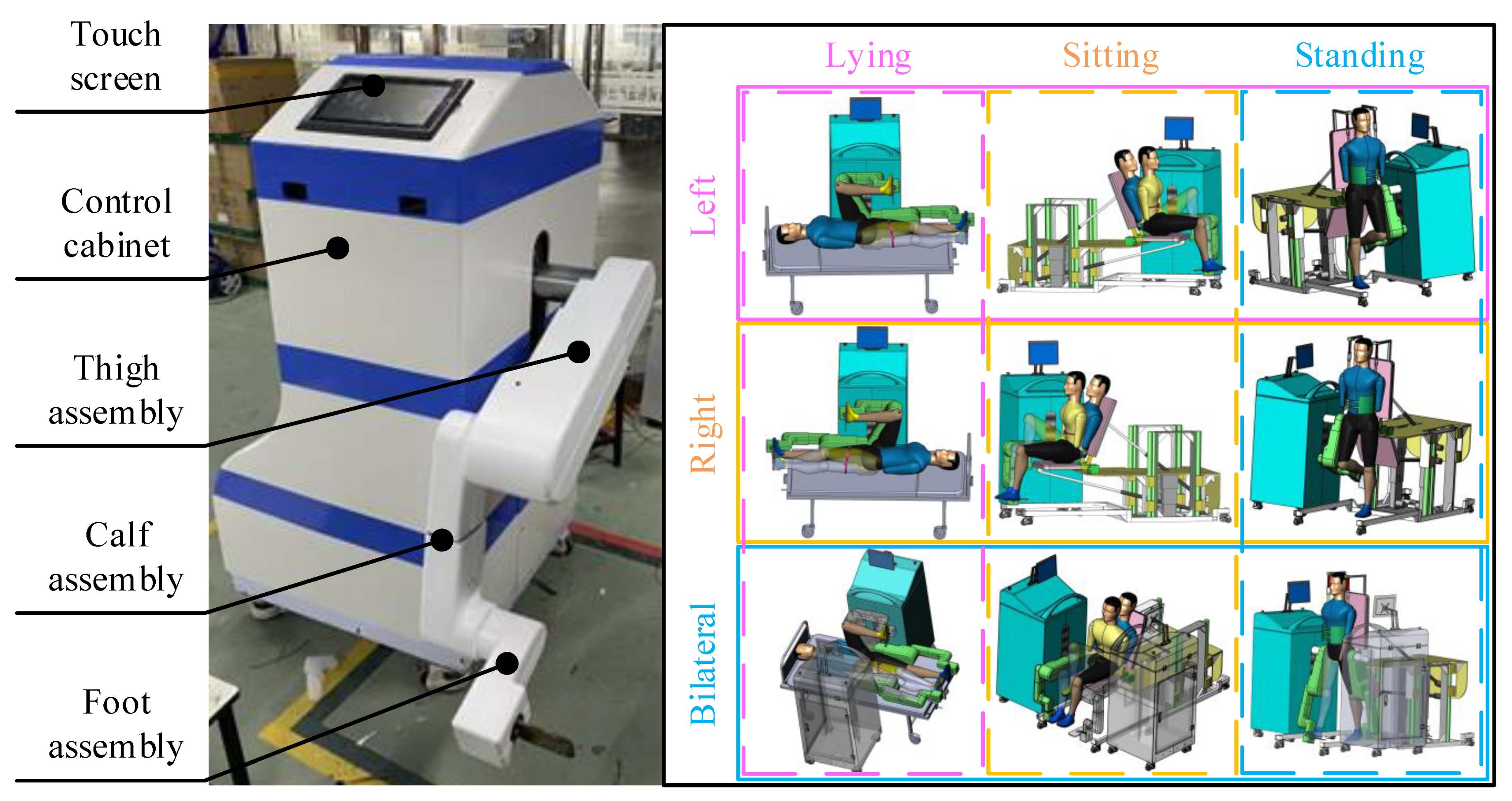
2.1. Overall Structure
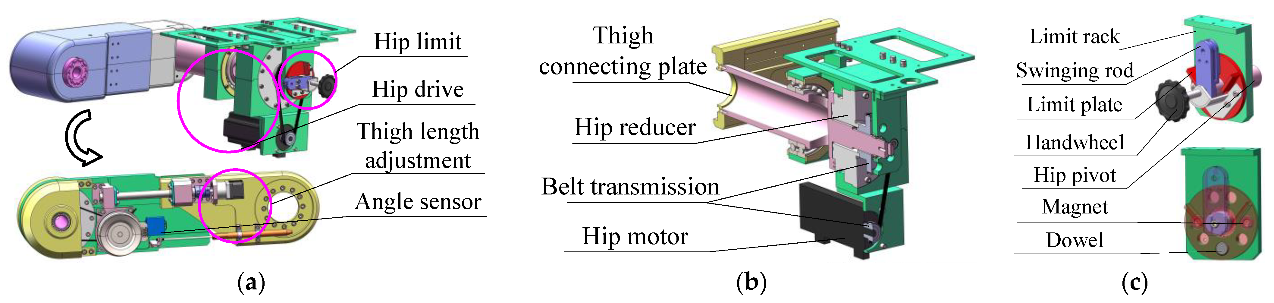
2.2. Thigh Assembly
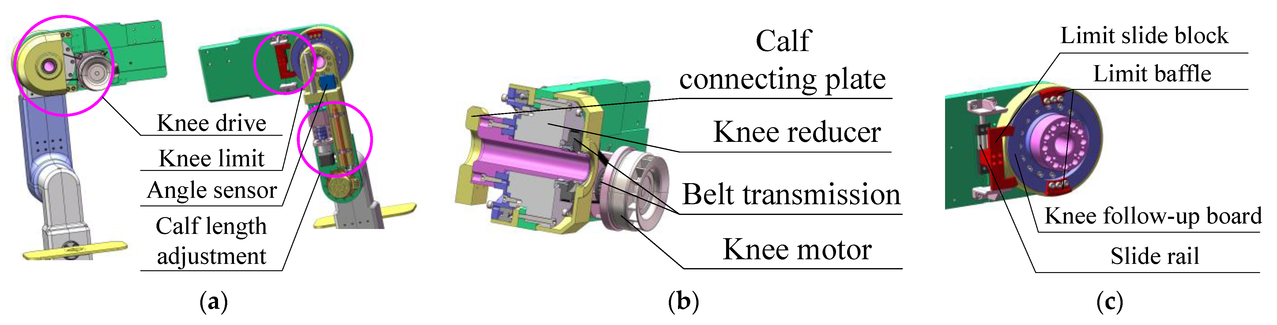
2.3. Calf Assembly
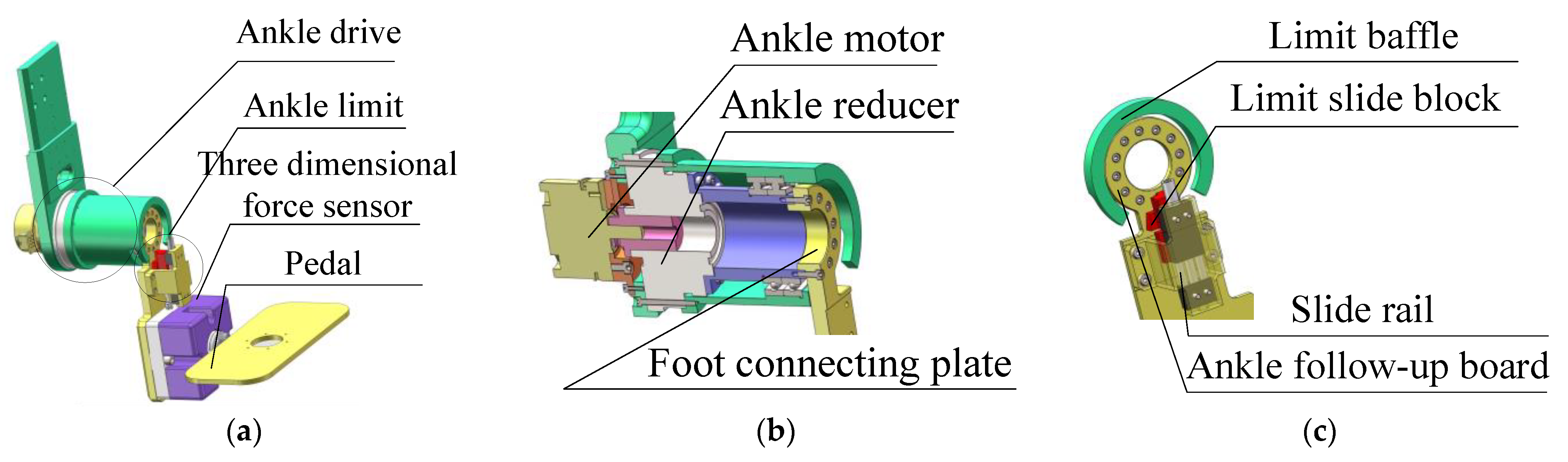
2.4. Foot Assembly
3. Gait Trajectory Planning Based on the Gait Models
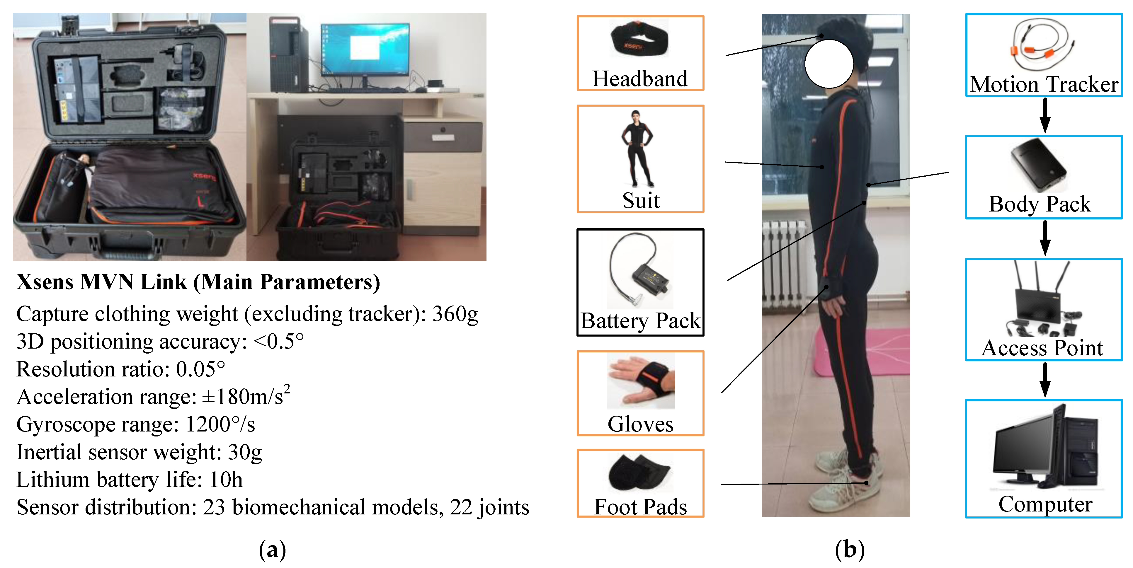
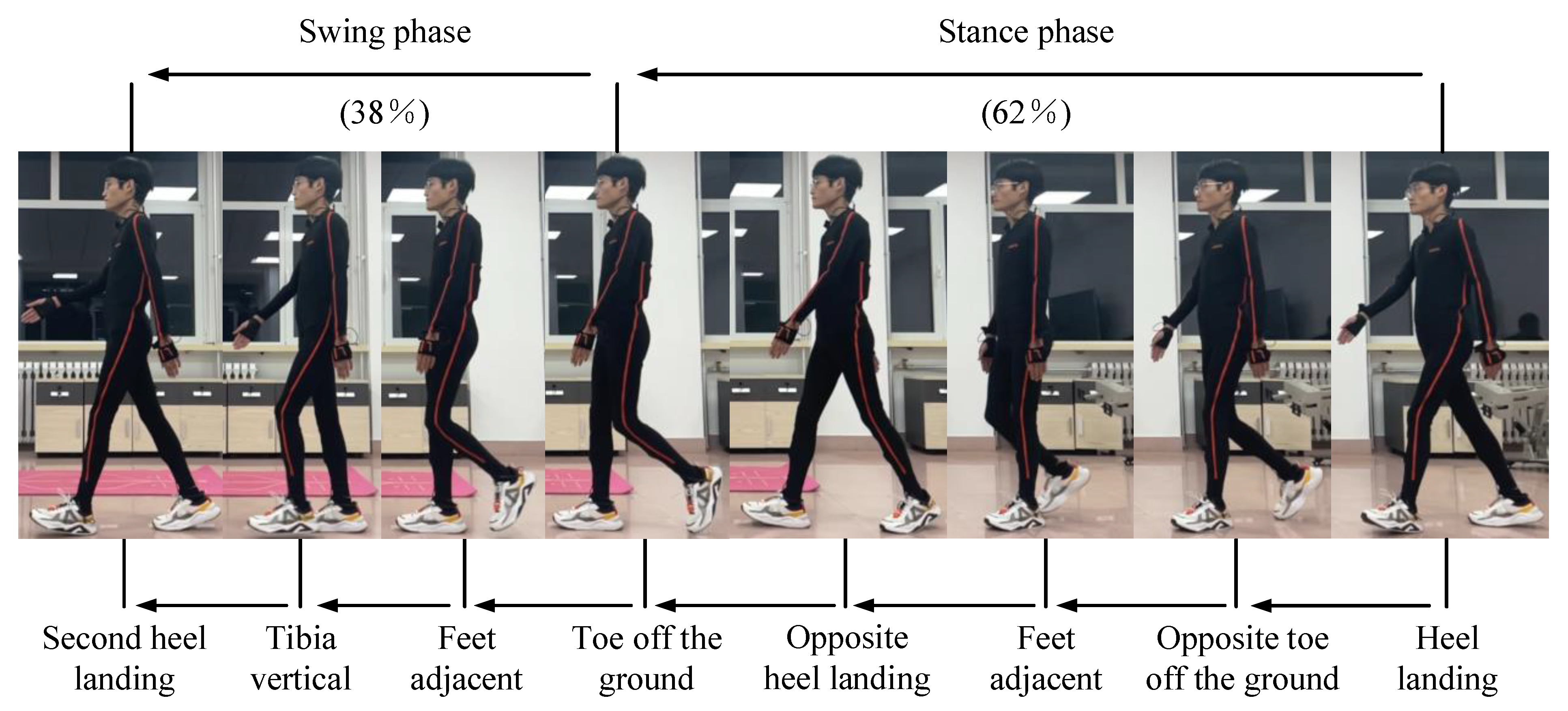
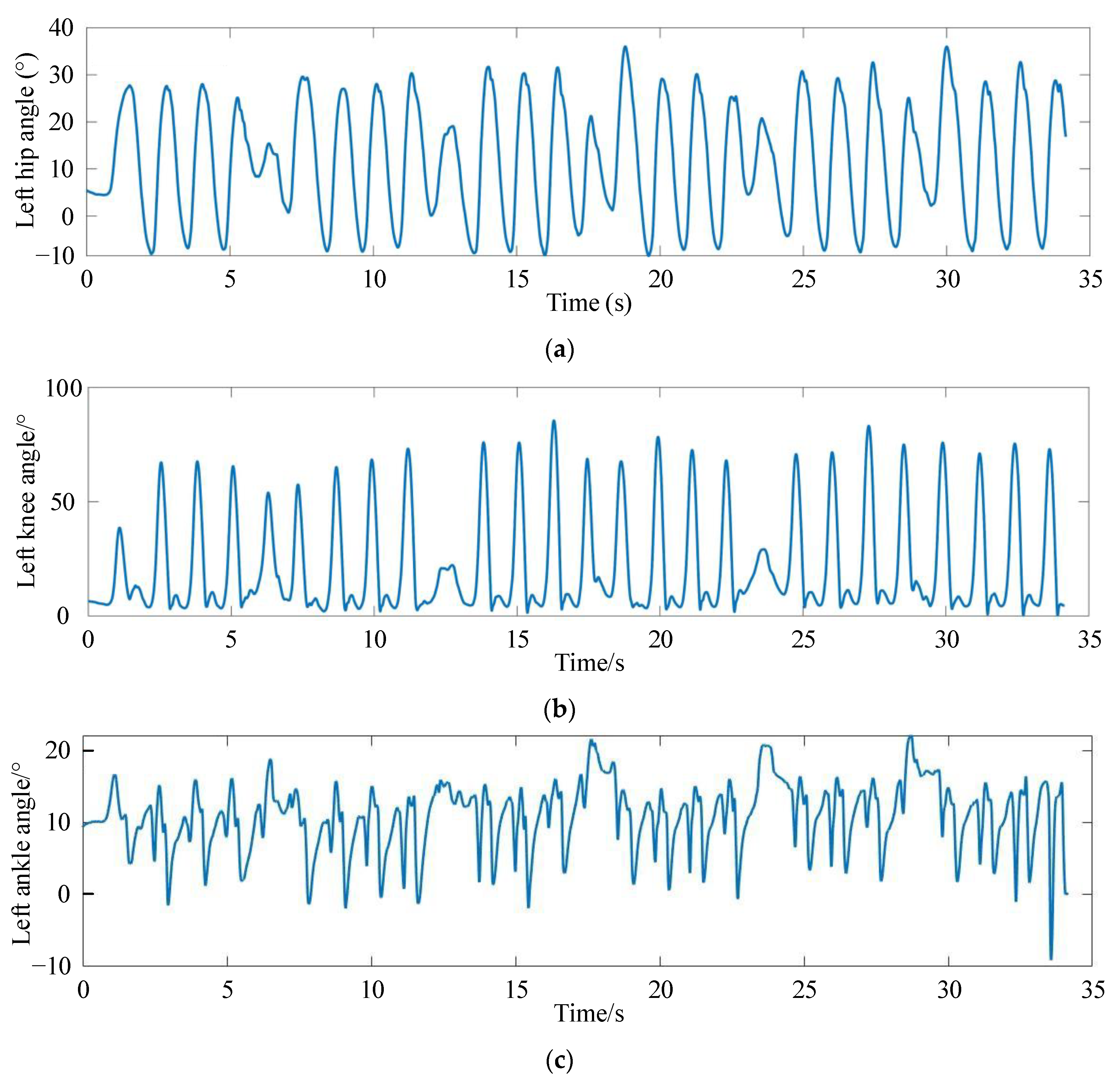
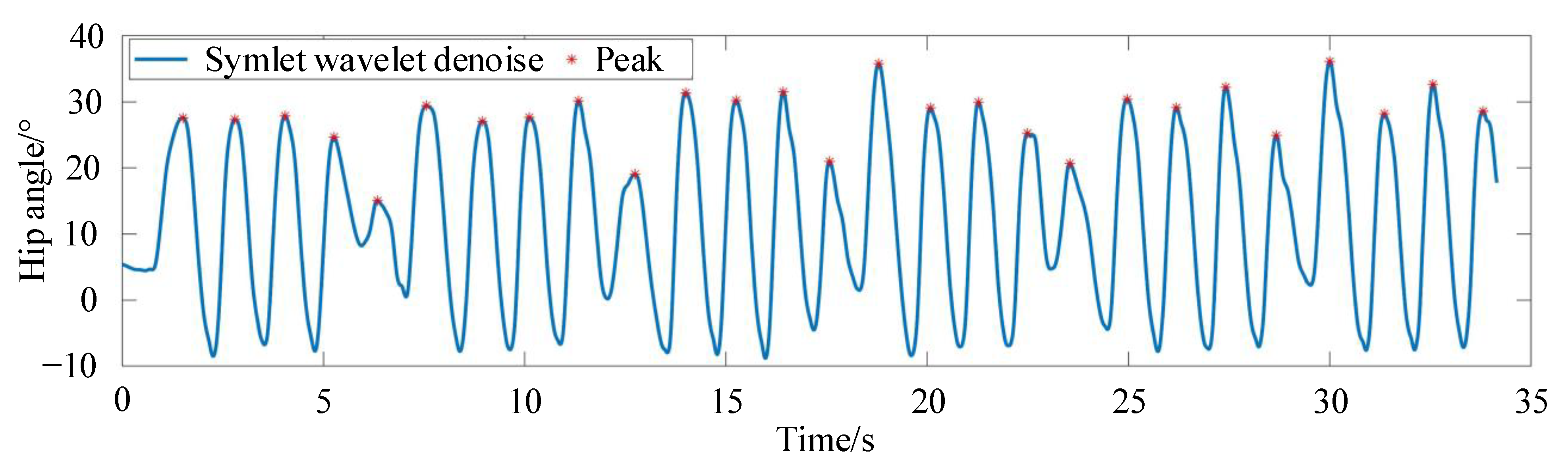
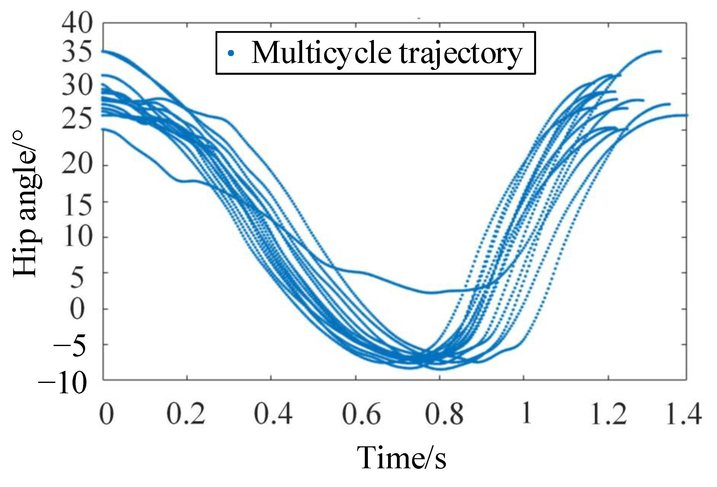
3.1. Gait Trajectory Collection
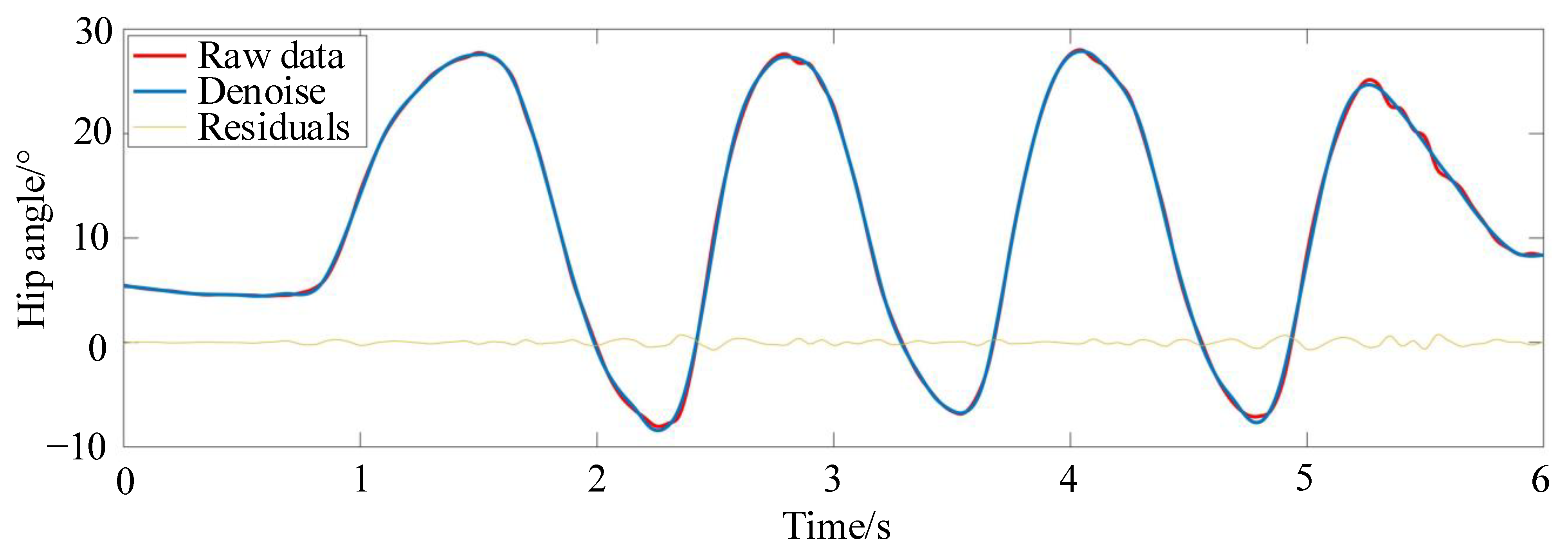
3.2. Periodic Information Extraction
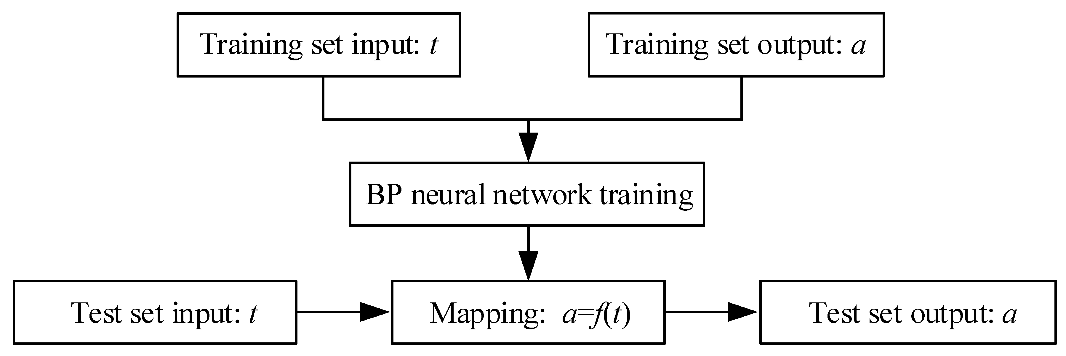
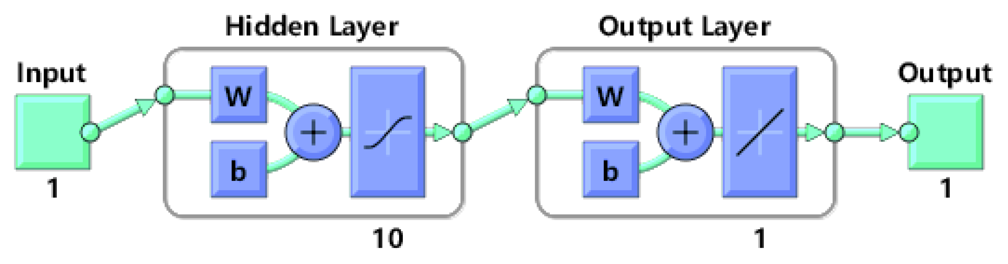
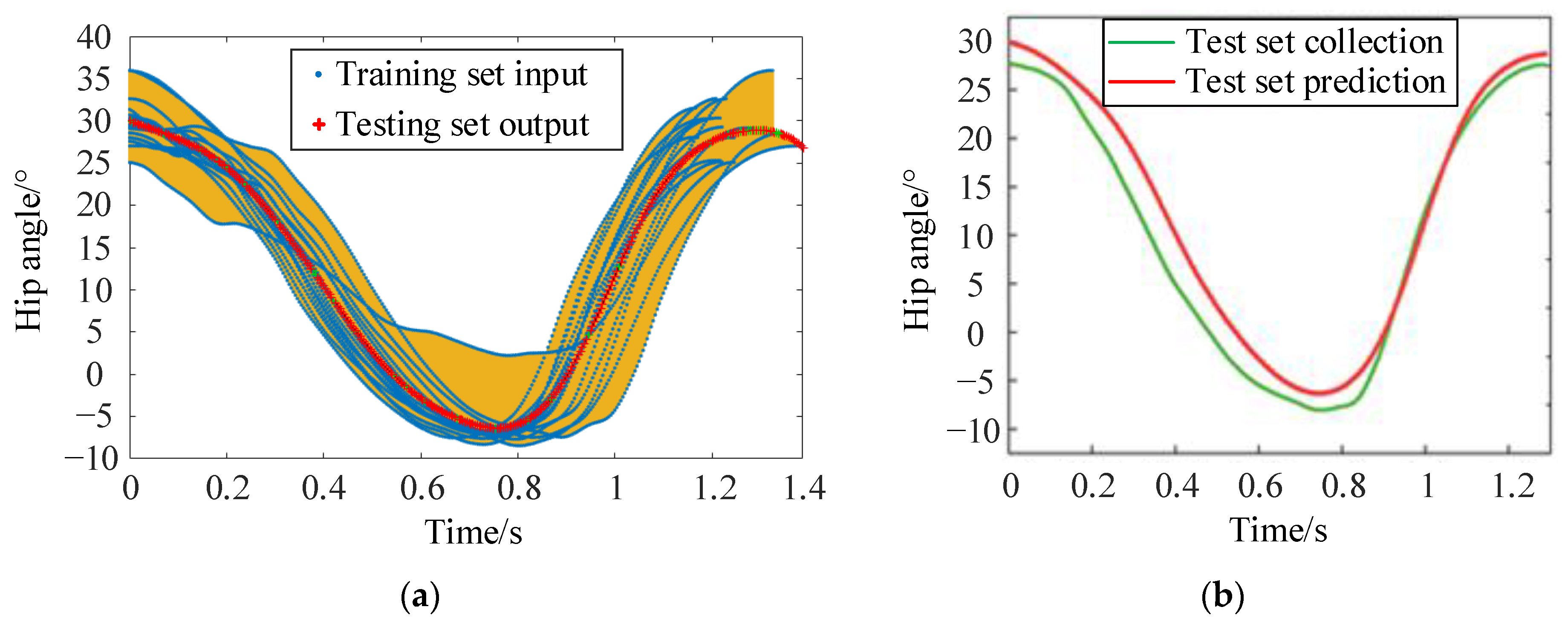
3.3. BP Neural Network Calibration
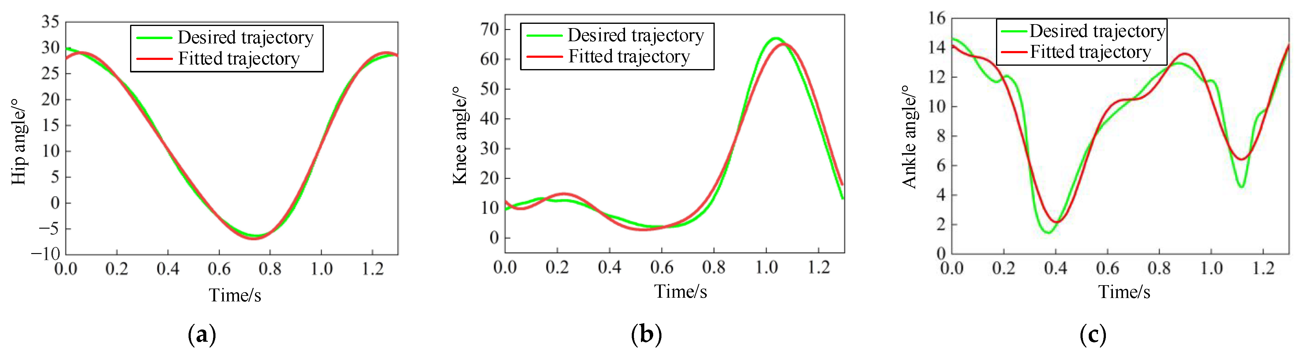
3.4. Fourier Function Curve Fitting
3.5. Digital Model Accuracy Verification
4. Gait Trajectory Tracking
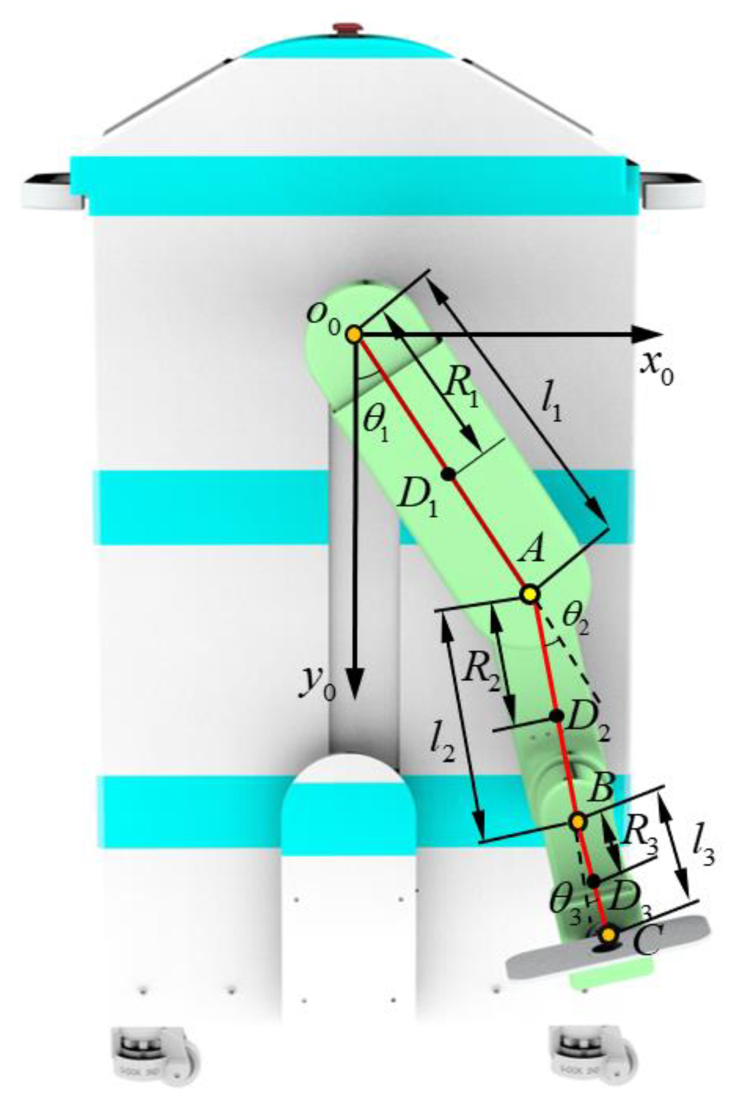
4.1. Dynamic Modeling of the MHLRR
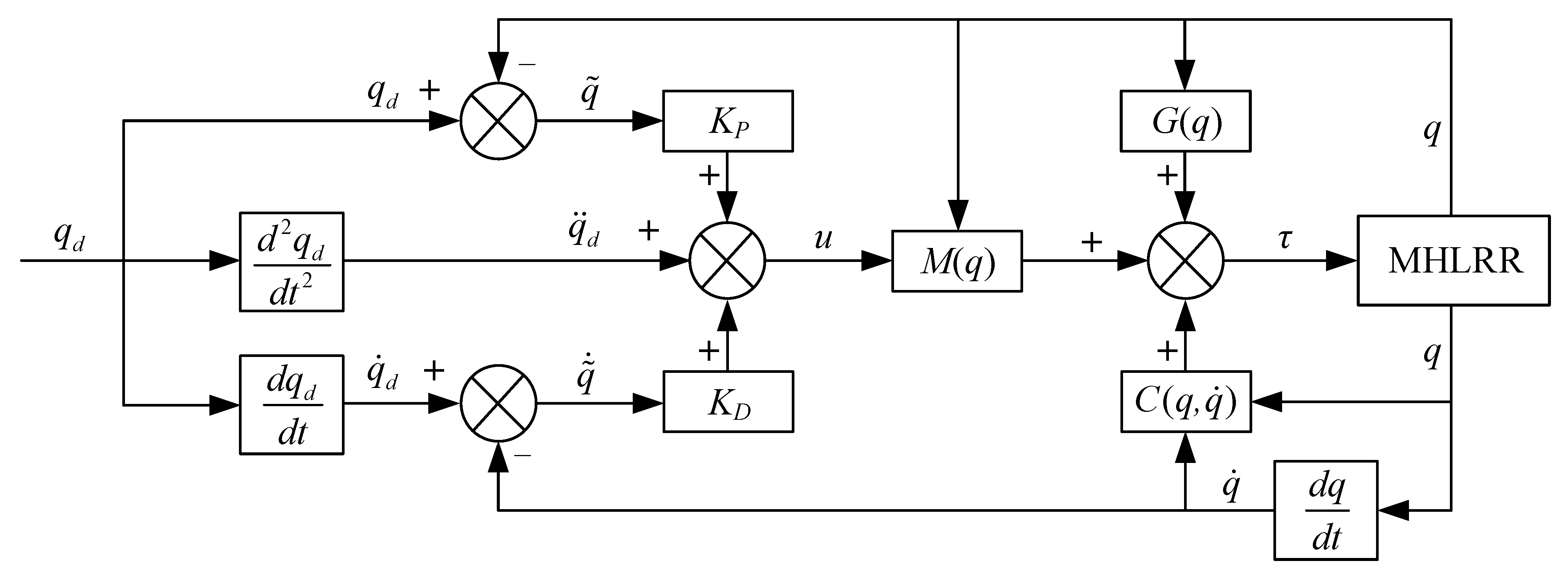
4.2. Controller Design for Adaptive Trajectory Tracking
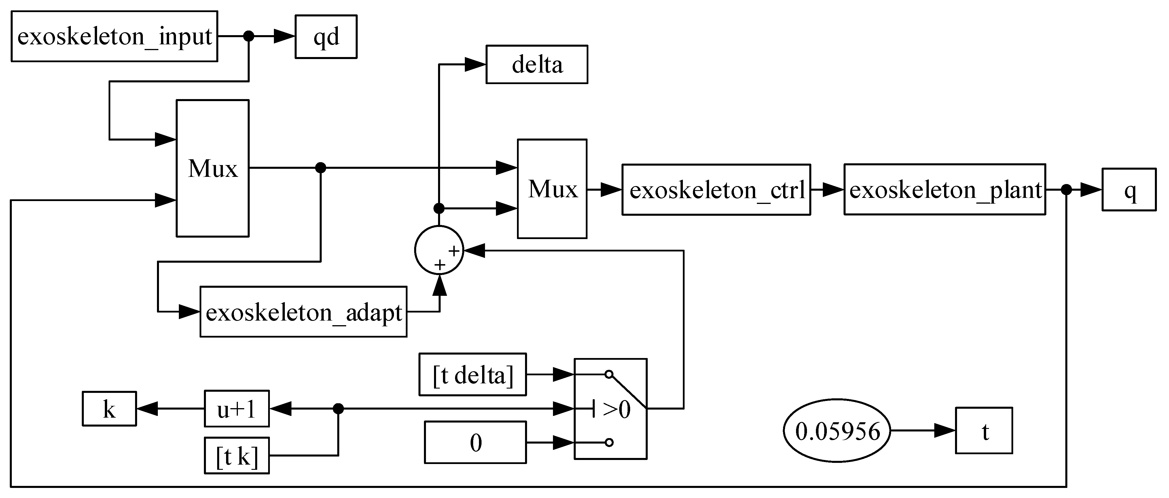
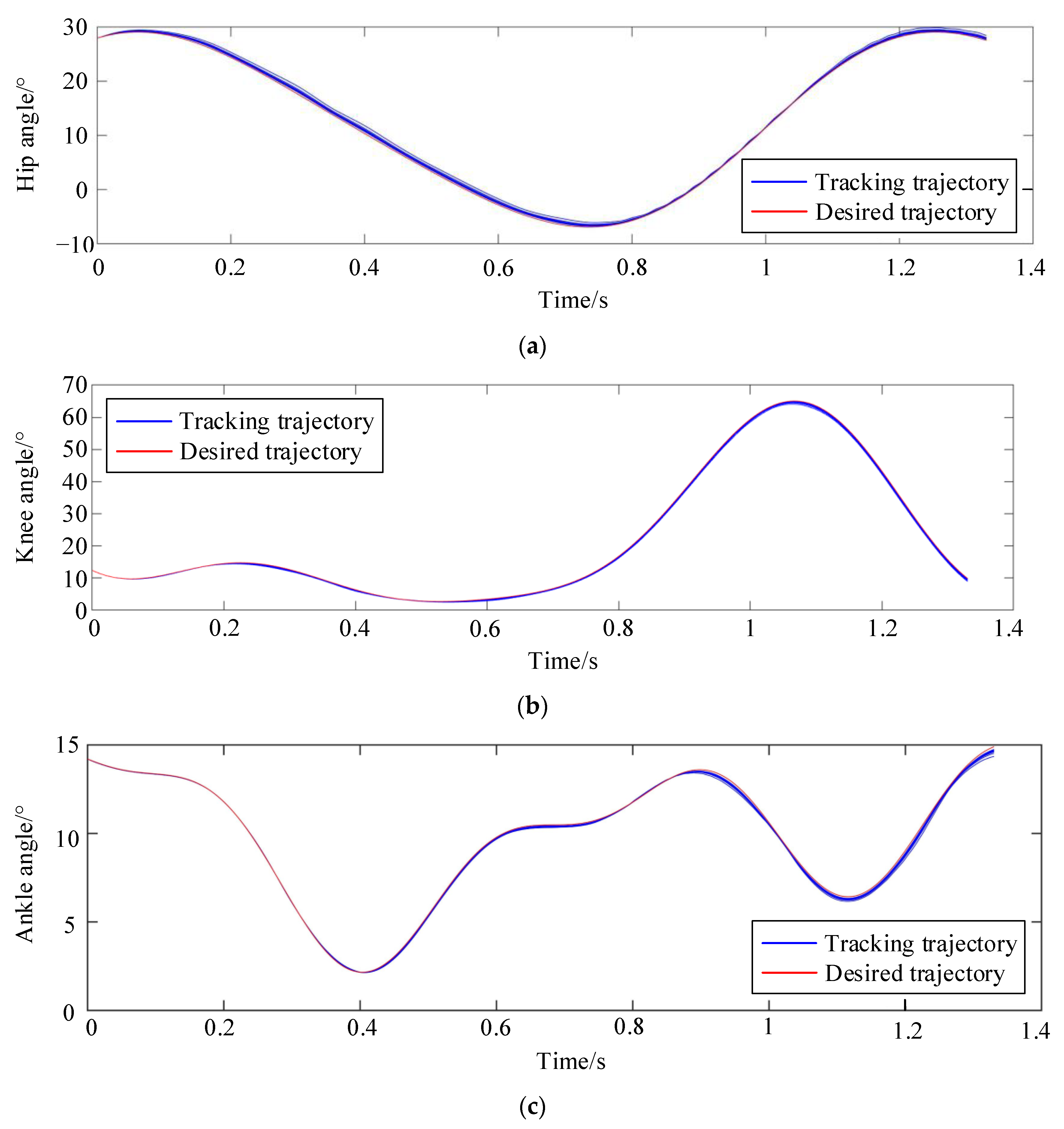
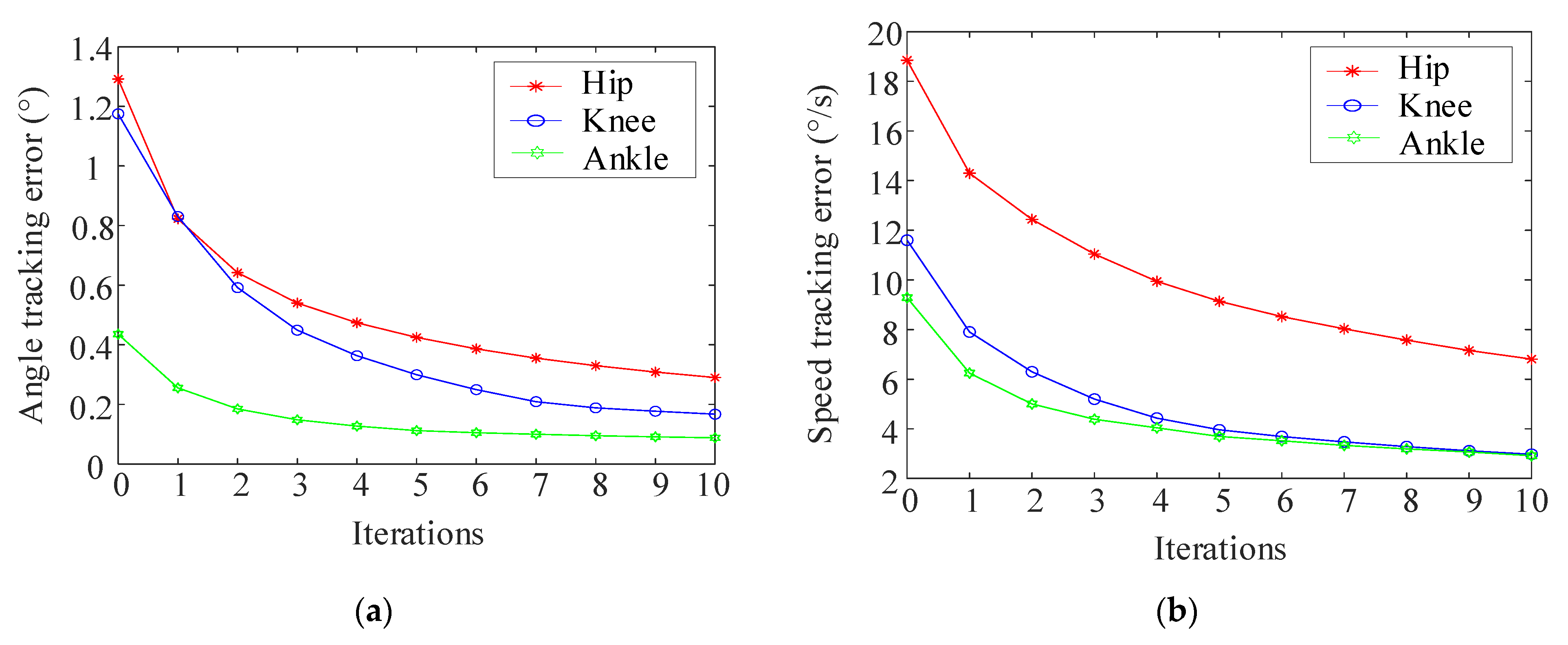
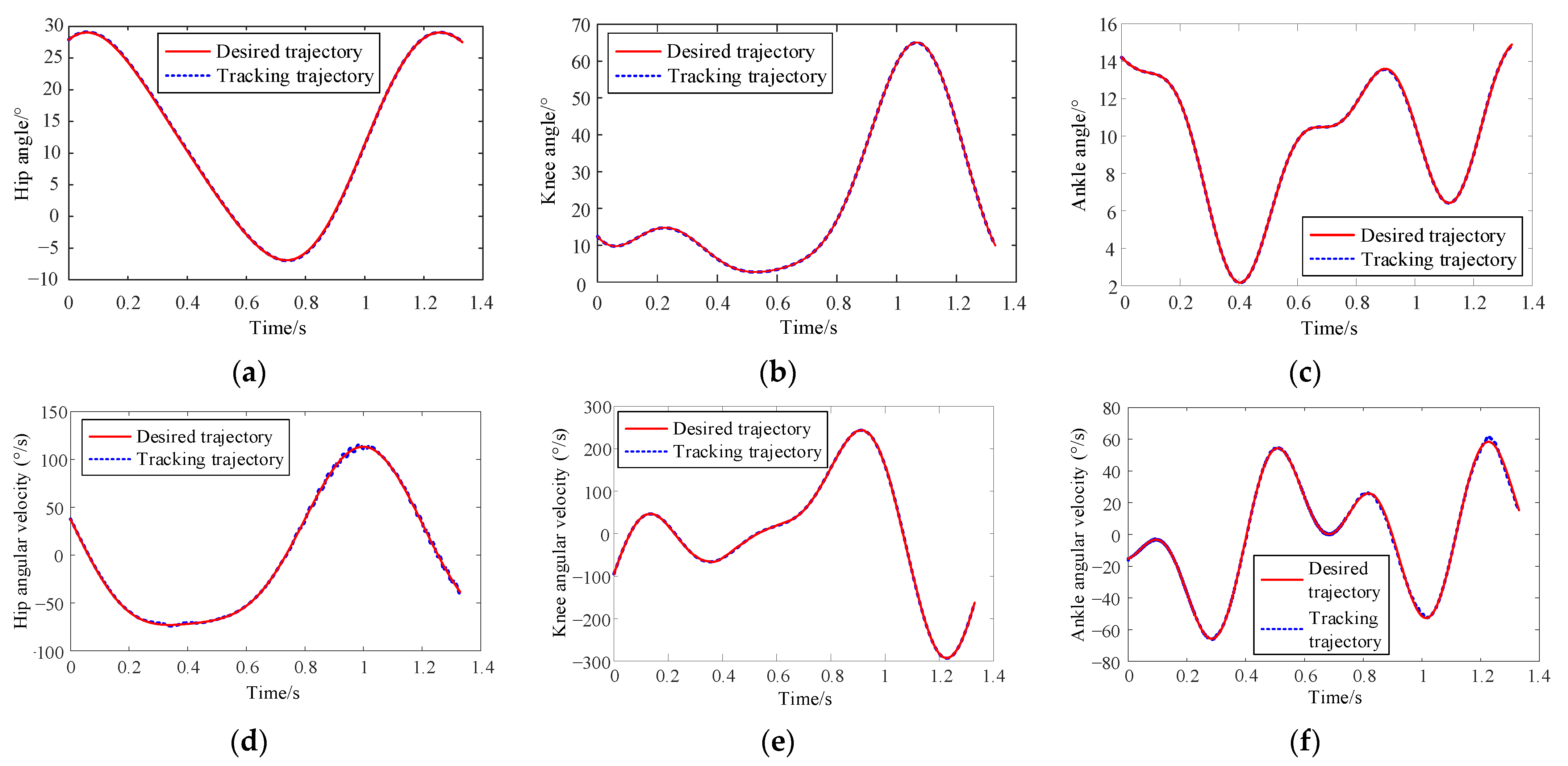
4.3. Simulation of Adaptive Trajectory Tracking
5. Experiment
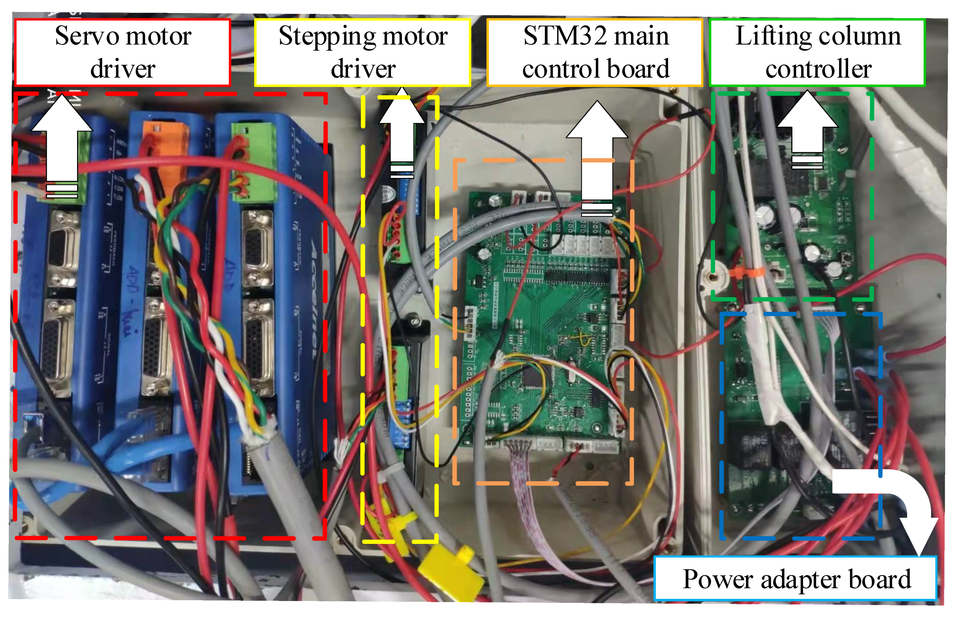
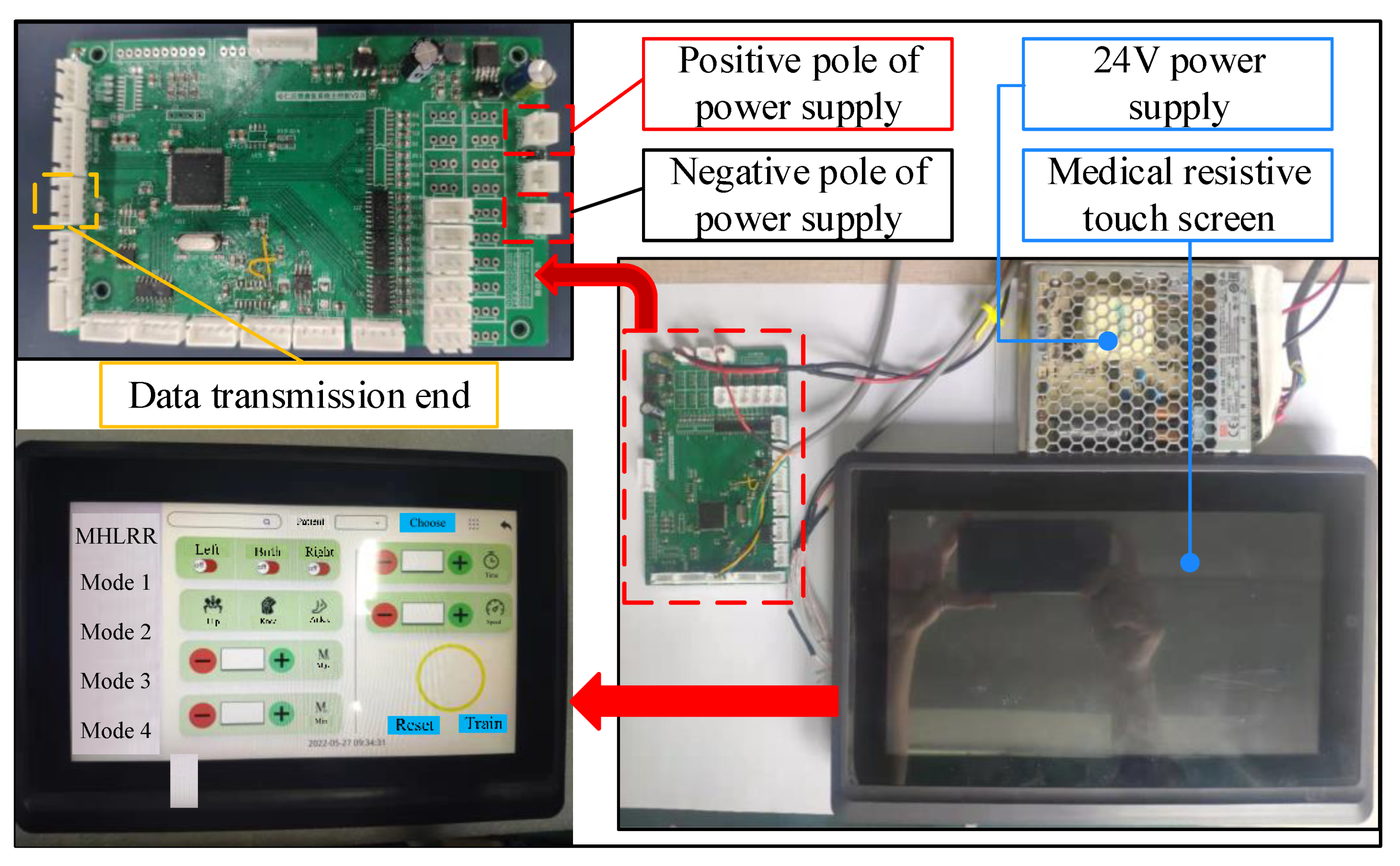
5.1. Experimental Platform
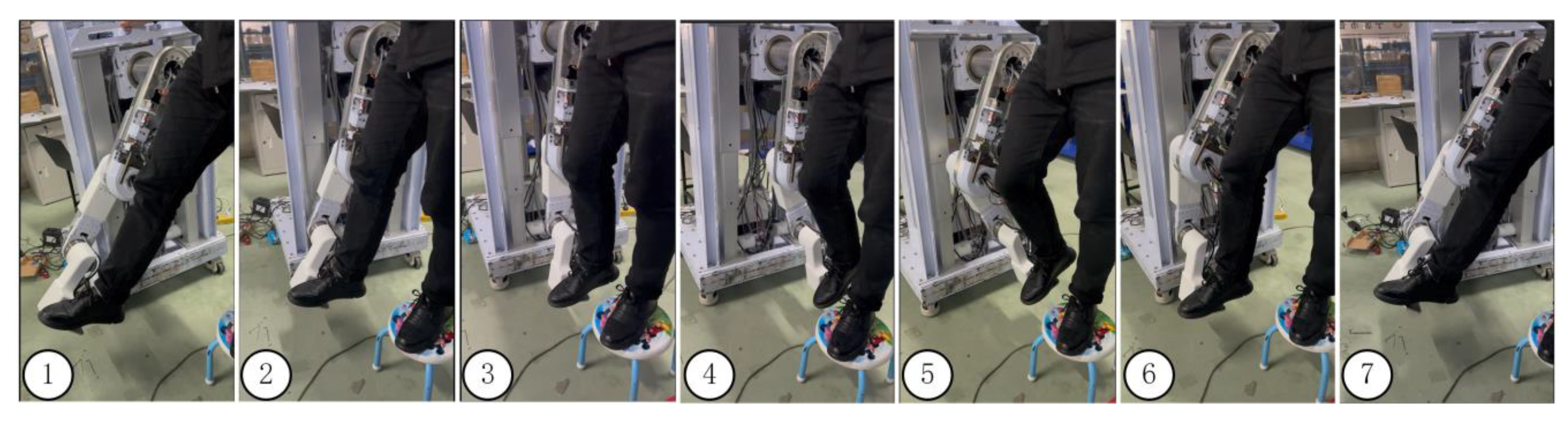
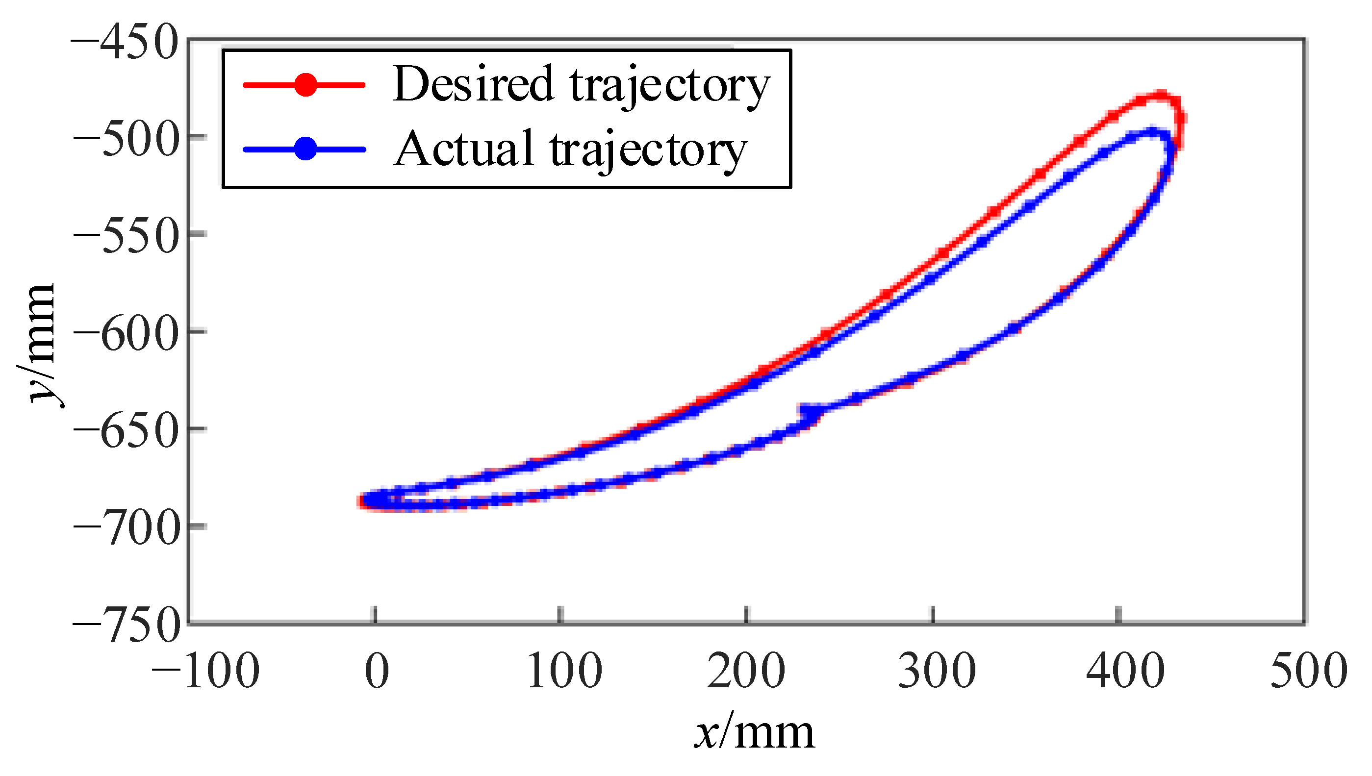
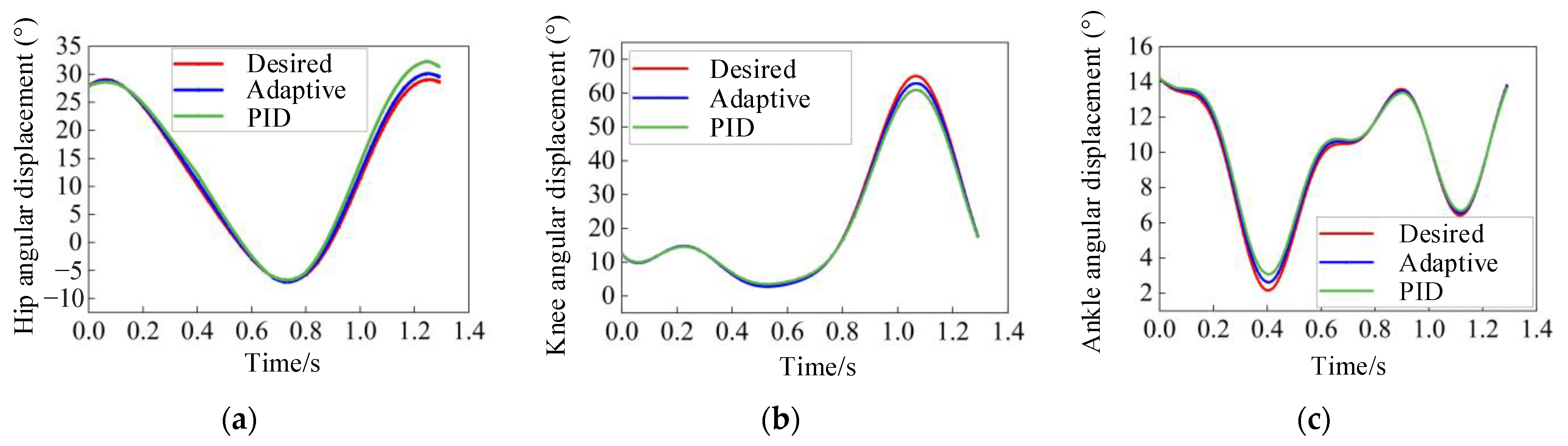
5.2. Gait Trajectory Tracking
6. Conclusions and Future Work
Author Contributions
Funding
Institutional Review Board Statement
Informed Consent Statement
Data Availability Statement
Conflicts of Interest
References
- Markus, H.S. Reducing disability after stroke. Int. J. Stroke 2022, 17, 249–250. [Google Scholar] [CrossRef] [PubMed]
- Feigin, V.L.; Nguyen, G.; Cercy, K.; Johnson, C.O.; Alam, T.; Parmar, P.G.; Abajobir, A.A.; Abate, K.H.; Abd-Allah, F.; Abejie, A.N. Global, Regional, and Country-Specific Lifetime Risks of Stroke, 1990 and 2016. N. Engl. J. Med. 2018, 379, 2429–2437. [Google Scholar] [PubMed]
- Feigin, V.L.; Stark, B.A.; Johnson, C.O.; Roth, G.A.; Bisignano, C.; Abady, G.G.; Hamidi, S. Global, regional, and national burden of stroke and its risk factors, 1990–2019: A systematic analysis for the Global Burden of Disease Study 2019. Lancet Neurol. 2021, 20, 795–820. [Google Scholar] [CrossRef]
- Flansbjer, U.B.; Holmbck, A.M.; Downham, D.; Patten, C.; Lexell, J. Reliability of gait performance in men and women with hemiparesis after stroke. J. Rehabil. Med. 2005, 37, 75–82. [Google Scholar] [PubMed]
- Sunilkumar, P.; Mohan, S.; Mohanta, J.K.; Wenger, P.; Rybak, L. Design and motion control scheme of a new stationary trainer to perform lower limb rehabilitation therapies on hip and knee joints. Int. J. Adv. Robot. Syst. 2022, 19, 172988142210751. [Google Scholar] [CrossRef]
- Ming, F.; Foong, R.; Yu, H. A Supine Gait Training Device for Stroke Rehabilitation. ASME J. Med. Devices 2014, 8, 020926. [Google Scholar] [CrossRef]
- Guzman-Valdivia, C.H.; Blanco-Ortega, A.; Oliver-Salazar, M.A.; Gomez-Becerra, F.A.; Carrera-Escobedo, J.L. HipBot—The design, development and control of a therapeutic robot for hip rehabilitation. Mechatronics 2015, 30, 55–64. [Google Scholar] [CrossRef]
- Komada, S.; Hashimoto, Y.; Okuyama, N.; Hisada, T.; Hirai, J. Development of a Biofeedback Therapeutic-Exercise-Supporting Manipulator. IEEE Trans. Ind. Electron. 2009, 56, 3914–3920. [Google Scholar] [CrossRef]
- Schmitt, C.; Métrailler, P.; AI-Khodairy, A.; Brodard, R.; Clavel, R. The Motion Maker™: A Rehabilitation System Combining an Orthosis with Closed-Loop Electrical Muscle Stimulation. In Proceedings of the 8th Vienna International Workshop on Functional Electrical Stimulation, Vienna, Austria, 27 January 2004. [Google Scholar] [CrossRef]
- Metrailler, P.; Blanchard, V.; Perrin, I.; Brodard, R.; Frischknecht, R.; Schmitt, C.; Fournier, J.; Bouri, M.; Clavel, R. Improvement of rehabilitation possibilities with the MotionMaker. In Proceedings of the First IEEE/RAS-EMBS International Conference on Biomedical Robotics and Biomechatronics, Pisa, Italy, 20–22 February 2006. [Google Scholar] [CrossRef]
- Wang, X.; Wang, H.; Hu, X.; Tian, Y.; Lin, M.; Yan, H.; Niu, J.; Sun, L. Adaptive Direct Teaching Control with Variable Load of the Lower Limb Rehabilitation Robot (LLR-II). Machines 2021, 9, 142. [Google Scholar] [CrossRef]
- Zhang, F.; Hou, Z.G.; Cheng, L.; Wang, W.Q.; Chen, Y.X.; Hu, J.; Peng, L.; Wang, H.B. iLeg—A lower limb rehabilitation robot: A proof of concept. IEEE Trans. Hum.-Mach. Syst. 2016, 46, 761–768. [Google Scholar] [CrossRef]
- Akdogan, E.; Adli, M.A. The design and control of a therapeutic exercise robot for lower limb rehabilitation: Physiotherabot. Mechatronics 2011, 21, 509–522. [Google Scholar] [CrossRef]
- Chisholm, K.J.; Klumper, K.; Mullins, A.; Ahmadi, M. A task oriented haptic gait rehabilitation robot. Mechatronics 2014, 24, 1083–1091. [Google Scholar] [CrossRef]
- Tomisaki, H. Development of portable therapeutic exercise machine TEM LX2 type D. In 36th International Symposium on Robotics Symposium Digest; Keidanren Kaikan: Tokyo, Japan, 2005. [Google Scholar]
- Daunoraviciene, K.; Adomaviciene, A.; Svirskis, D.; Griskevicius, J.; Juocevicius, A. Necessity of early-stage verticalization in patients with brain and spinal cord injuries: Preliminary study. Technol. Health Care 2018, 26, S613–S623. [Google Scholar] [CrossRef] [PubMed]
- Pérez, V.Z.; Yepes, J.C.; Vargas, J.F.; Franco, J.C.; Escobar, N.I.; Betancur, L.; Sánchez, J.; Betancur, M.J. Virtual Reality Game for Physical and Emotional Rehabilitation of Landmine Victims. Sensors 2022, 22, 5602. [Google Scholar] [CrossRef] [PubMed]
- Yepes, J.C.; Portela, M.A.; Saldarriaga, J.; Pérez, V.Z.; Betancur, M.J. Myoelectric control algorithm for robot-assisted therapy: A hardware-in-the-loop simulation study. Biomed. Eng. Online 2019, 18, 3. [Google Scholar] [CrossRef] [PubMed]
- Hidler, J.; Wisman, W.; Neckel, N. Kinematic trajectories while walking within the Lokomat robotic gait-orthosis. Clin. Biomech. 2008, 23, 1251–1259. [Google Scholar] [CrossRef] [PubMed]
- Fleerkotte, B.M.; Koopman, B.; Buurke, J.H.; van Asseldonk, E.H.F.; van der Kooij, H.; Rietman, J.S. The effect of impedance-controlled robotic gait training on walking ability and quality in individuals with chronic incomplete spinal cord injury: An explorative study. J. NeuroEng. Rehabil. 2014, 11, 26. [Google Scholar] [CrossRef] [PubMed]
- Veneman, J.F.; Kruidhof, R.; Hekman, E.E.G.; Ekkelenkamp, R.; Van Asseldonk, E.H.F.; van der Kooij, H. Design and evaluation of the LOPES exoskeleton robot for interactive gait rehabilitation. IEEE Trans. Neural Syst. Rehabil. Eng. 2007, 15, 379–386. [Google Scholar] [CrossRef] [PubMed]
- Banala, S.K.; Kim, S.H.; Agrawal, S.K.; Scholz, J.P. Robot Assisted Gait Training with Active Leg Exoskeleton (ALEX). IEEE Trans. Neural Syst. Rehabil. Eng. 2009, 17, 2–8. [Google Scholar] [CrossRef]
- Winfree, K.N.; Stegall, P.; Agrawal, S.K. Design of a minimally constraining, passively supported gait training exoskeleton: ALEX II. In Proceedings of the 2011 IEEE International Conference on Rehabilitation Robotics, Zurich, Switzerland, 29 June–1 July 2011. [Google Scholar]
- Freivogel, S.; Mehrholz, J.; Husak-Sotomayor, T.; Schmalohr, D. Gait training with the newly developed ‘LokoHelp’-system is feasible for non-ambulatory patients after stroke, spinal cord and brain injury, A feasibility study. Brain Inj. 2008, 22, 625–632. [Google Scholar] [CrossRef]
- Freivogel, S.; Schmalohr, D.; Mehrholz, J. Improved walking ability and reduced therapeutic stress with an electromechanical gait device. J. Rehabil. Med. 2009, 41, 734–739. [Google Scholar] [CrossRef] [PubMed]
- Stauffer, Y.; Allemand, Y.; Bouri, M.; Fournier, J.; Clavel, R.; Metrailler, P.; Brodard, R.; Reynard, F. The WalkTrainer-A New Generation of Walking Reeducation Device Combining Orthoses and Muscle Stimulation. IEEE Trans. Neural Syst. Rehabil. Eng. 2009, 17, 38–45. [Google Scholar] [CrossRef] [PubMed]
- Luu, T.P.; Low, K.H.; Qu, X.; Lim, H.B.; Hoon, K.H. Hardware Development and Locomotion Control Strategy for an Over-Ground Gait Trainer: NaTUre-Gaits. IEEE J. Transl. Eng. Health Med.-JTEHM 2014, 2, 2100209. [Google Scholar] [CrossRef] [PubMed]
- Strausser, K.A.; Swift, T.A.; Zoss, A.B.; Kazerooni, H.; Bennett, B.C. Mobile exoskeleton for spinal cord injury: Development and testing. In Proceedings of the ASME Dynamic Systems and Control Conference and Bath/ASME Symposium on Fluid Power and Motion Control (DSCC 2011), Arlington, VA, USA, 31 October–2 November 2011. [Google Scholar]
- Ogata, T.; Abe, H.; Samura, K.; Hamada, O.; Nonaka, M.; Iwaasa, M.; Higashi, T.; Fukuda, H.; Shiota, E.; Tsuboi, Y.; et al. Hybrid Assistive Limb (HAL) Rehabilitation in Patients with Acute Hemorrhagic Stroke. Neurol. Med.-Chir. 2015, 55, 901–906. [Google Scholar] [CrossRef] [PubMed]
- Rose, L.; Bazzocchi, M.C.F.; de Souza, C.; Vaughan-Graham, J.; Patterson, K.; Nejat, G. A framework for mapping and controlling exoskeleton gait patterns in both simulation and real-world. In Proceedings of the 2020 Design of Medical Devices Conference (DMD2020), Minneapolis, MN, USA, 6–9 April 2020. [Google Scholar]
- Fazel, R.; Shafei, A.M.; Nekoo, S.R. A new method for finding the proper initial conditions in passive locomotion of bipedal robotic systems. Commun. Nonlinear Sci. Numer. Simul. 2024, 130, 107693. [Google Scholar] [CrossRef]
- Added, E.; Gritli, H.; Belghith, S. Trajectory tracking-based control of the chaotic behavior in the passive bipedal compass-type robot. Eur. Phys. J.-Spec. Top. 2022, 231, 1071–1084. [Google Scholar] [CrossRef]
- Park, J.; Haan, J.; Park, F.C. Convex optimization algorithms for active balancing of humanoid robots. IEEE Trans. Robot. 2007, 23, 817–822. [Google Scholar] [CrossRef]
- Tayebi, A. Adaptive iterative learning control for robot manipulators. Automatica 2004, 40, 1195–1203. [Google Scholar] [CrossRef]


| Height | Shoulder Height | Hip Height | Knee Height | Ankle Height |
|---|---|---|---|---|
| 168 cm | 138 cm | 94 cm | 47 cm | 9 cm |
| Number | 1 | 2 | 3 | 4 | 5 | 6 |
| Cycle interval (s) | 1.512–2.8 | 2.8–4.046 | 4.046–5.263 | 7.558–8.946 | 8.046–10.12 | 10.12–11.34 |
| Number | 7 | 8 | 9 | 10 | 11 | 12 |
| Cycle interval (s) | 14–15.25 | 15.25–16.42 | 18.8–20.08 | 20.08–21.27 | 21.27–22.49 | 24.97–26.19 |
| Number | 13 | 14 | 15 | 16 | 17 | 18 |
| Cycle interval (s) | 26.19–27.42 | 27.42–28.67 | 28.67–30 | 30–31.35 | 31.35–32.56 | 32.56–33.81 |
| Number of Hidden Layer Nodes | Mean Absolute Error (MAE) | Mean Squared Error (MSE) | Root Mean Square Error (RMSE) |
|---|---|---|---|
| 5 | 2.3207 | 7.9289 | 2.8158 |
| 10 | 2.2851 | 7.6949 | 2.7740 |
| 15 | 2.3101 | 8.0051 | 2.8229 |
| Joint Angular Displacement | Fitting Times | Variance (SSE) | Root-Mean-Square (RMSE) | Correction Coefficient (R-Square) |
|---|---|---|---|---|
| Hip | 2 | 117 | 0.6203 | 0.9977 |
| Knee | 3 | 314.4 | 1.02 | 0.9976 |
| Ankle | 4 | 247.1 | 0.8872 | 0.9416 |
| Joint | Hip | Knee | Ankle |
|---|---|---|---|
| Motor Model | SMP8024 | NBL9040 | EC60 |
| Rated Power (W) | 382 | 335 | 150 |
| Rated Torque (N·m) | 1 | 0.9 | 0.401 |
| Rated Voltage (V) | 24 | 24 | 24 |
| Rated Speed (rpm) | 3650 | 4700 | 3480 |
| Reducer Model | HSG40 | HSG32 | HSG20 |
| Reduction Ratio | 100 | 100 | 100 |
| Rated Torque (N·m) | 345 | 178 | 52 |
Disclaimer/Publisher’s Note: The statements, opinions and data contained in all publications are solely those of the individual author(s) and contributor(s) and not of MDPI and/or the editor(s). MDPI and/or the editor(s) disclaim responsibility for any injury to people or property resulting from any ideas, methods, instructions or products referred to in the content. |
© 2024 by the authors. Licensee MDPI, Basel, Switzerland. This article is an open access article distributed under the terms and conditions of the Creative Commons Attribution (CC BY) license (https://creativecommons.org/licenses/by/4.0/).
Share and Cite
Wang, X.; Wang, H.; Zhang, B.; Zheng, D.; Yu, H.; Cheng, B.; Niu, J. A Multistage Hemiplegic Lower-Limb Rehabilitation Robot: Design and Gait Trajectory Planning. Sensors 2024, 24, 2310. https://doi.org/10.3390/s24072310
Wang X, Wang H, Zhang B, Zheng D, Yu H, Cheng B, Niu J. A Multistage Hemiplegic Lower-Limb Rehabilitation Robot: Design and Gait Trajectory Planning. Sensors. 2024; 24(7):2310. https://doi.org/10.3390/s24072310
Chicago/Turabian StyleWang, Xincheng, Hongbo Wang, Bo Zhang, Desheng Zheng, Hongfei Yu, Bo Cheng, and Jianye Niu. 2024. "A Multistage Hemiplegic Lower-Limb Rehabilitation Robot: Design and Gait Trajectory Planning" Sensors 24, no. 7: 2310. https://doi.org/10.3390/s24072310
APA StyleWang, X., Wang, H., Zhang, B., Zheng, D., Yu, H., Cheng, B., & Niu, J. (2024). A Multistage Hemiplegic Lower-Limb Rehabilitation Robot: Design and Gait Trajectory Planning. Sensors, 24(7), 2310. https://doi.org/10.3390/s24072310