3.1. Grey Correlation Analysis Based on SBAS-InSAR Deformation Analysis and Using Multiple Impact Factors
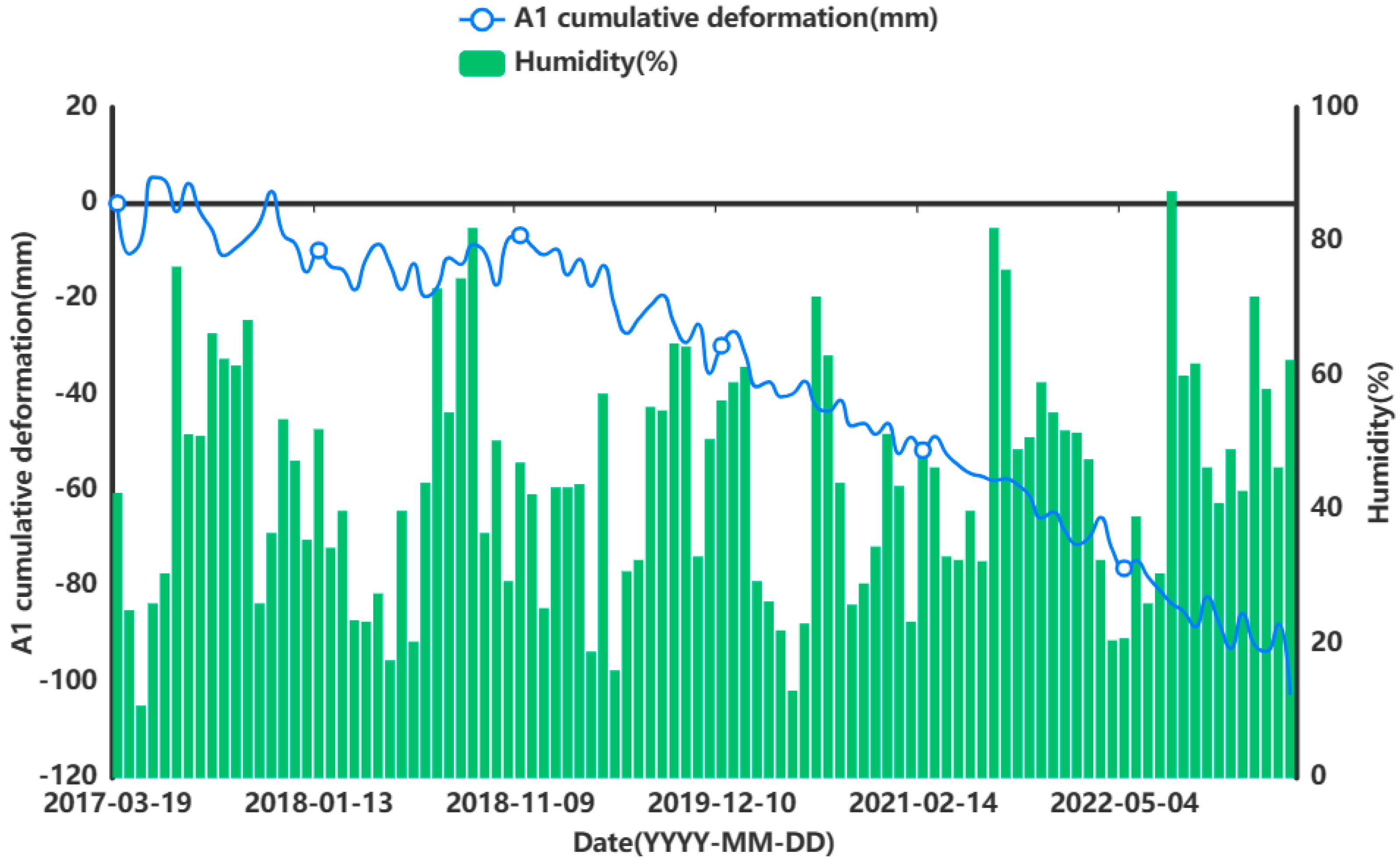
In order to prove that the influencing factors will affect the surface deformation of the city to a certain extent, and also indirectly prove that it is feasible to consider multiple factors in a prediction study of surface change, in this paper, we obtained the surface deformation data for the Hohhot urban area by using SBAS-InSAR (ENVI 5.3) technology and used grey correlation to analyse the correlation degree between multiple factors and the surface changes.
The SBAS-InSAR technique [
21,
22,
23,
24] performs deformation measurements by means of a small baseline differential interferometric atlas, which can reduce the influence of spatial de-correlation and terrain errors, and then applies the singular value decomposition (SVD) method based on the least-paradigm criterion of the deformation rate to obtain the deformation rate of coherent targets and their time series [
25]. Its technological flow is shown in
Figure 2.
In this paper, SBAS-InSAR processing is performed on 100-view Sentinel-1A radar image data [
26,
27]. The specific data processing steps are as follows:
- (1)
Interferometric connectivity map generation. By means of interferometric image pair pairing of 100-view image data, the 15 January 2020 image is selected as the super-controller image, the SAR image is optimally combined to form a short baseline set, and the generated spatio-temporal baseline condition is shown in
Figure 3a,b. The interferogram controller sub-image is sorted in chronological order to obtain the controller–client image sequence,
,
, and
; all the differential interferograms can be combined into a system of observation equations:
- (2)
Differential interference workflow. After the aligning, deplaning, and topographic phase processing of interfering pairs, adaptive filtering is used to consistently phase out noise and obtain smooth differential interferograms. Then, phase de-entanglement is carried out using the least-cost flow method, and interfering pairs with poor coherence or de-entangled phase transitions are rejected and re-decomposed.
- (3)
Orbital refinement and re-delevelling. A reference point (the GCP point) is selected as the orbit refinement control point, and the GCP point is used to estimate and remove the residual constant phase, as well as the phase ramps that remain after unwrapping. The GCP reference point is shown in
Figure 4.
- (4)
Deformation rate and DEM coefficient estimation. The differential phase of any image element (x, y) on the kth interferogram can be simplified by using a polynomial model to assist the external DEM for orbit refinement and re-deplaning, removing the terrain phase and ignoring the noise and other phases (see Equation (2)). The deformation and elevation information of all image pairs are inverted based on the linear model to estimate the deformation rate and residual terrain phase. This is shown in Equation (3).
- (5)
Atmospheric phase and terrain residual phase removal. Atmospheric delayed phases are estimated and removed using spatio-temporal filtering, and orbital error residual phases are updated to separate line-of-sight deformation information, as shown in Equation (4).
- (6)
Geocoding. Geocoding the SBAS results after atmospheric correction, the final deformation rate information is obtained for 539,184 points, and the obtained surface deformation results are shown in
Figure 5.
PS-InSAR is a surface deformation monitoring technique that uses multi-scene SAR imagery of the same area to analyse scattering points that are coherent and stable over time, in terms of time series amplitude and phase, and are not easily affected by spatial and temporal incoherence factors [
28]. Through the main and auxiliary imaging standards, differential interference SAR image processing uses the primary digital elevation model (DEM) to remove the terrain phase, generate the interference atlas, use the amplitude separation index to select the candidate point and use the three-dimensional diluted separation network to solve the phase. The nonlinear deformation and the atmosphere are separated through time- and space-domain filtering, and finally, the millimetre-level surface transformation information is obtained through geographical coding.
In order to verify the correctness of the InSAR results, the PS-InSAR technology obtains the surface transformation data of the research area, and the 963 settings of the same name are selected to compare the data with SBAS-InSAR for comparative verification. The surface transformation of the PS-InSAR technology is shown in
Figure 6, and the correlation analysis plot between PS-InSAR and SBAS-InSAR is shown in
Figure 7.
The results from the above comparison analysis prove that the surface transformation data that were obtained using SBAS-InSAR technology in the research area are reliable.
Grey correlation analysis is based on grey correlation by comparing the degree of similarity between the geometric relationship of the data series and the geometric shape of the curve. It is an analytical method that can be used to analyse the degree of correlation between factors of a system by assessing the relative strength of the influence of a certain item compared with the other factors in the grey system [
29]. The key steps are as follows:
Determine the multi-column matrix data that affect the behaviour of the system, as shown in Equation (5).
To exclude the impact of the difference between the units of each indicator and their value in the order of magnitude of the disparity that is brought about by the phenomenon of irrationality, reduce the absolute value of the data differences. A dimensionless matrix holds the initial value in this method, as well as the average value, etc., and in this paper, the initial value of the dimensionless matrix is calculated as shown in Equation (6).
Calculate the difference sequence, the absolute difference between the corresponding elements of each evaluated object’s indicator sequence (comparison sequence), and the pre-reference sequence, as shown in Equation (7).
Calculate the maximum and minimum difference between the two levels, as shown in Equation (8).
Calculate the grey correlation coefficient, as shown in Equation (9).
where
,
,
is the discrimination coefficient of the degree of association between the balanced indicators of the model, using values within (0, 1). The larger the value is, the smaller the difference between the coefficients of association is, and the weaker the ability to distinguish, generally 0.5, will be.
To calculate the grey correlation degree, since the grey correlation coefficient (
) is used to evaluate the degree of relationship between different levels of each factor and the standard indicators, the difference in the grey correlation coefficients of different levels of the same factor results in a more dispersed evaluation of the factor’s degree of influence on the system as a whole [
30]. Therefore, the average value of the grey correlation coefficients at different levels of the factors is usually taken to be the quantitative value for evaluating the degree of association between the original factor columns and the standard columns, as shown in Equation (10).
3.2. Surface Deformation Prediction Model Based on SSA-CNN-LSTM Neural Network
The SSA-CNN-LSTM model is a multi-influence surface deformation prediction model constructed by using the SSA, CNN, and LSTM neural network [
31,
32]. Combining the fast optimisation parameter search of the SSA, the strong feature information extraction function of the CNN, and the short-term fine prediction capability of the LSTM model, the optimal parameter values are searched for by the SSA. Ultimately, the purpose of minimising the prediction value error of the CNN-LSTM model is achieved, and the prediction accuracy is improved. As shown in
Figure 8, the specific steps of the SSA-CNN-LSTM neural network prediction model are as follows:
- (1)
Data preparation and analysis stage: The SBAS-InSAR technique was used to acquire time series surface deformation data in the study area. The air temperature, humidity, precipitation, and ground temperature at 5 cm, 10 cm, and 15 cm below the surface in the study area were used as input data, and the time series cumulative surface deformation data at the feature points were used as the output. The acquired data were normalized to remove the effect of magnitude, and the data were chemically divided, including 70 groups for the training set, 21 groups for the test set, and 9 groups for the validation set.
- (2)
SSA parameter optimisation phase: Initialise the number of sparrow populations, update the sparrow population position, determine the quantitative evaluation method of adaptation, and calculate the adaptation value and the adaptation function. Input the data into the CNN-LSTM network, construct the network structure, randomly initialise the network weights as inputs for the SSA algorithm, initialise the sparrow population, divide the population into discoverers and followers, and then under the influence of the optimal search of the network hyperparameters, continuously update the network by updating the discoverer position and follower position. Update the randomly selected vigilantes and update the position to determine whether the optimal hyperparameter iteration stopping condition is satisfied. If so, obtain the optimal hyperparameters of the CNN-LSTM network. Otherwise, go back to the division of the population again. The SSA is used to obtain the optimal learning rate, number of hidden nodes, and regularisation coefficients and constraints in the CNN-LSTM model. Among them, the parameters of the sparrow search algorithm are shown in
Table 2.
- (3)
Predictive modelling stage: Randomly initialise the network weights and transfer the optimal network hyperparameters that were obtained by means of the SSA to the CNN-LSTM model, which decodes these to obtain the optimal values of the learning rate, hidden nodes, and regularisation coefficients. The optimised convolutional layer performs feature extraction on the input data, inputs them into the LSTM layer for feature extraction, updates the weights of the entire neural network model, determines whether it meets the accuracy requirements or reaches the maximum number of iterations, and if it does not meet the iterative stopping conditions, then the convolutional layer returns to the parameter optimisation step and re-processes to ensure that it meets the conditions and ultimately obtains the timing prediction results. The main SSA-CNN-LSTM parameter settings are shown in
Table 3.
The SSA algorithm can be used to control the movement position between the sparrow and the food according to the fitness value, which increases with the number of iterations, thus achieving an iterative optimisation of the food structure and the optimal solution of the global problem. Using this approach, the final optimised network model and parameters can be obtained by passing different input data through the convolutional and LSTM layers, respectively. The CNN extracts the features from different input data, while the LSTM layer learns the features that have been extracted by the CNN and then inputs the output features into the fully connected layer for prediction. The training set that is obtained from data processing is used for network simulation training, and finally, the test set data are predicted to derive the error between the predicted output value and the actual value. In this process, the value of the SSA fitness function is continuously reduced to minimise the mean square error with the increase in the number of iterations, and the resulting network model is optimal, which in turn minimises the error between the predicted value and the true value [
33,
34].
The SSA is a global optimisation algorithm based on the foraging and anti-predation activities of sparrow populations [
19]. It has significant advantages in terms of convergence speed and convergence accuracy. The basic idea of the sparrow search algorithm is to optimise the parameters by dividing the population, updating the guidance mechanism for the population’s location, determining the optimal food source according to the fitness function, and finally, determining the global optimal parameters.
Discoverers provide a foraging direction for the population and guidance for followers, and the location updates are shown in Equation (11).
where
is the number of iterations,
is the preset maximum number of iterations,
and
denote the position of the sparrow at time t and at time t + 1, respectively, after the update,
is a random number in [0, 1], and
is the alarm threshold. When
, it indicates that the sparrow is discovering, entering search mode, and updating its location. When
, it indicates that the vigilant in the population has detected a danger and the discoverer stops foraging at this time and flies to a safe location.
The identities of discoverers and followers will shift, but the proportion of both in the population is fixed, there are no predators in the foraging environment, and the producers can perform the optimal search and provide optimal guidance to the joiners. The first m sparrows with high adaptation in each generation are discoverers,
n-m sparrows are followers, and the follower’s position is updated as shown in Equation (12).
where
is the worst position in the global search of the population,
is the optimal position in the population at the current moment, and
is a dimensional matrix with elements with random values of −1 or 1.
In the sparrow population, the initial positions of all sparrows are randomly generated. Assuming that a small percentage of sparrows will be aware of the danger and will quickly move closer to their surrounding companions to reduce the risk of their own predation, the position of this category of sparrows is updated as shown in Equation (13).
where
is the global optimal position at the current moment,
is a parameter that obeys a normal distribution and is used for step size control,
is a random number within
,
is a constant that avoids a denominator of 0,
is the value of the fitness function,
is the current optimal fitness value,
is the current worst fitness value, and
indicates that the population is centred and secure within a certain range around it. When
, the sparrows at the edge of the population are aware of the risk, and when
, it indicates that the sparrows in the middle of the population are moving closer to their peers.
The minimum mean squared error (MSE) between the prediction set and the validation set is taken as the condition for the iterative termination of the SSA algorithm in order to find the optimal parameters, as shown in Equation (14).
where
is the predicted value of the moment
obtained after network training,
is the true value of moment
in the validation set, and
is the length of the time series.
The network model searches for a set of hyperparameters that have the optimal fitness function to minimise the training error of the network based on the iterative variation in the MSE. The smaller the value of the MSE is, the better the predictive performance is, indicating that the model has a higher degree of accuracy.
A CNN is a deep feed-forward neural network structural model, designed and developed based on inspiration from biological visual nerves [
35,
36], and the model of its basic constituent unit structure is shown in
Figure 9.
In this paper, the DenseNet network structure is used as the CNN backbone network to extract the features of the input data. DenseNet adopts multiple DenseBlock connections, 2D convolution is selected, the dense connection between the convolutional layers is established by the feature cascade within each DenseBlock, and the main convolutional unit within the DenseBlock module is the BN-ReLU-Conv cascade, where BN (batch normalisation) is the batch normalisation layer, ReLU (Rectified Linear Unit) is the linear rectification activation layer, and Conv is the convolutional layer. The LSTM neural network goes through an input stage, a selective memory stage, and an output stage. Its CNN-LSTM neural network prediction model flow is as follows:
The convolutional layer is applied to the 2D input by sliding the convolution layer to create a dot product using the input matrix and the convolution kernel, as shown in Equation (15).
where
is the original data input matrix and
is the convolution kernel.
In order to solve the problem of size reduction of the output matrix of the data input data matrix I after the operation of the convolutional layer, data padding (padding) is applied to the matrix before the input convolutional layer. Let the size of the matrix before convolution be and the size of the convolution kernel be . The amplitude of the padding is set to . Then, the output of the convolved matrix is . Ensure that the size of the matrix before and after the convolution remains the same size.
The output matrix of each layer is the feature matrix, and the area that is covered by each element in the window of the convolution kernel of the original input matrix is referred to as the sensory field, as shown in Equation (16).
where
and
are the convolutional kernel window’s shift step and the convolutional kernel’s size for the corresponding layer
, respectively.
Pooling layer: After the data pass through the pooling layer, the pooling layer performs a pooling operation on the data and uses the statistical characteristics of the pooling window area, such as the maximum value or the average value, to represent the value of the entire pooling window, which is essentially a down sampling of the input data and reduces the size of the data. This can reduce the complexity of the feature computation and prevent overfitting during model training, and it enhances the robustness of the network.
The Flat Layer collapses the spatial dimension of the input into a channel dimension, facilitating its transition to a fully connected layer.
The fully connected layer comes after the convolutional layer and the pooling layer and is mainly used to map the learned features to the sample space and retain the complexity of the model to some extent.
Output layer: the output is performed using the softmax function (MATLAB R2022b), as shown in Equation (17).
A linear function was used to fit the predictions, as shown in Equation (18).
The learning method used is the Stochastic Gradient Descent (SGD), with the following basic steps:
- (1)
Initialise the parameters and weights of all the convolution kernels in the network.
- (2)
Input the data and perform the forward steps (convolution, activation, pooling, and fully connected forward propagation).
- (3)
Calculate the output layer error.
- (4)
Calculate the gradient of the error relative to the weights using the backpropagation algorithm, and reduce and update the parameters and weights of all convolutional kernels using gradient descent. Return to step (3) to calculate the error of the output layer and keep looping until the iteration stops by satisfying the limit difference.
LSTM is a kind of neural network with a unique time series processing ability in order to prevent the problem of gradient disappearance and the explosion of a recurrent neural network, the core of which lies in the forgetting gate, input gate, and output gate, which is able to make full use of the historical time series data and capture the temporal features in the data, as well as selectively retaining and forgetting the information to predict the future data more accurately [
37,
38,
39,
40]. The structure of its network model unit is shown in
Figure 10.
Building of LSTM feature learning layer: Learning the correlation between the time series and the sequence data, the features that were extracted from the CNN are fed into the LSTM layer for learning.
Input phase: Selective forgetting of information from the previous moment’s input message is performed [
41]. Whether the input is forgotten or not is controlled by the forgetting gating
, which controls the previous moment’s cell state,
. It is obtained by multiplying the splice vector
of the hidden state
of the previous moment and the input value
of the current moment by means of the weight matrix, followed by the bias term
, and then by an activation function
; the function is shown in
Figure 11.
is the control gate with a value range of 0 to 1, which is used to forget and retain the information, and
represents the weighting matrix for forgetting stages
and
.
represents the forgotten information from the previous state .
The selective memory stage decides to selectively “remember” the input information at the current moment, enhancing the memory of important information and reducing the memory of unimportant information [
42], while generating candidate cell states through the tanh function. The tanh function is shown in
Figure 12 and is used to prevent the gradient from exploding or vanishing.
denotes the input gating, and
determines the information enhancement.
represents the information that is enhanced by the current input content.
The outcome of passing the next node is obtained by adding the results that were obtained in the forgetting and selective memory stages (see Equation (24)).
The output phase determines the output information of the current cell state [
43]. The sigmoid layer is run first to compute the output gate, and then, the output cell state
that passed to the next node is multiplied by the tanh activation function to multiply the original output information pair-by-pair to obtain the final output (see Equation (25)) and the hidden state (see Equation (26)).
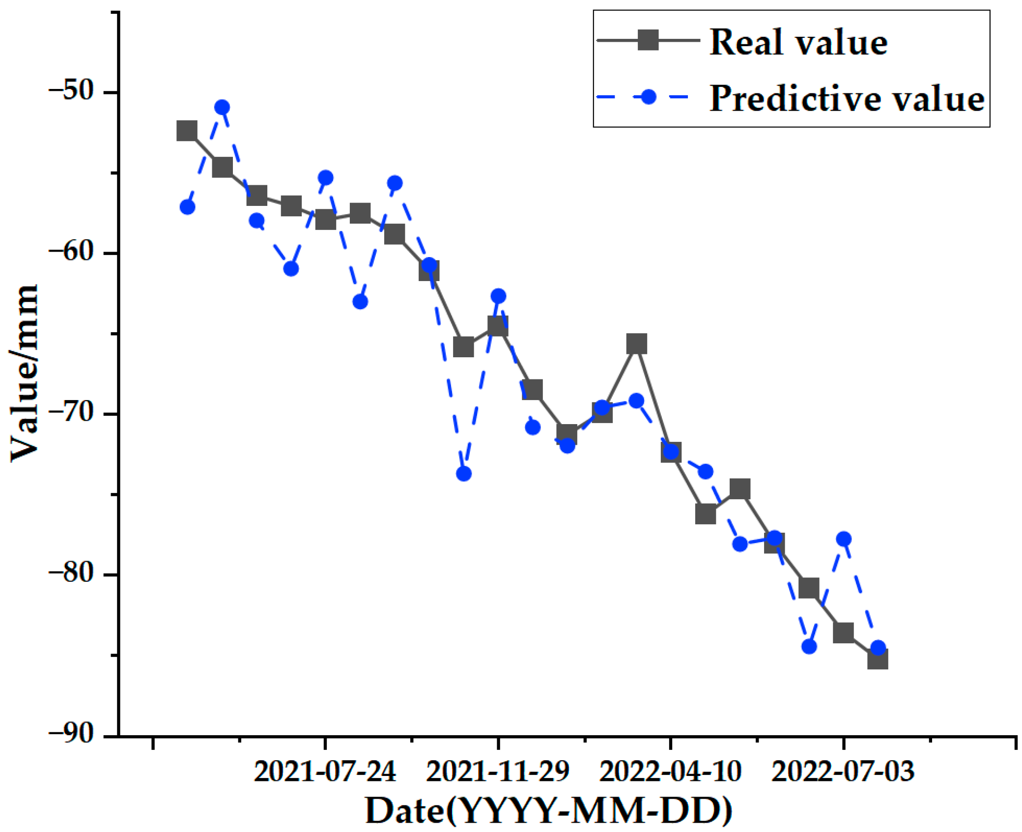
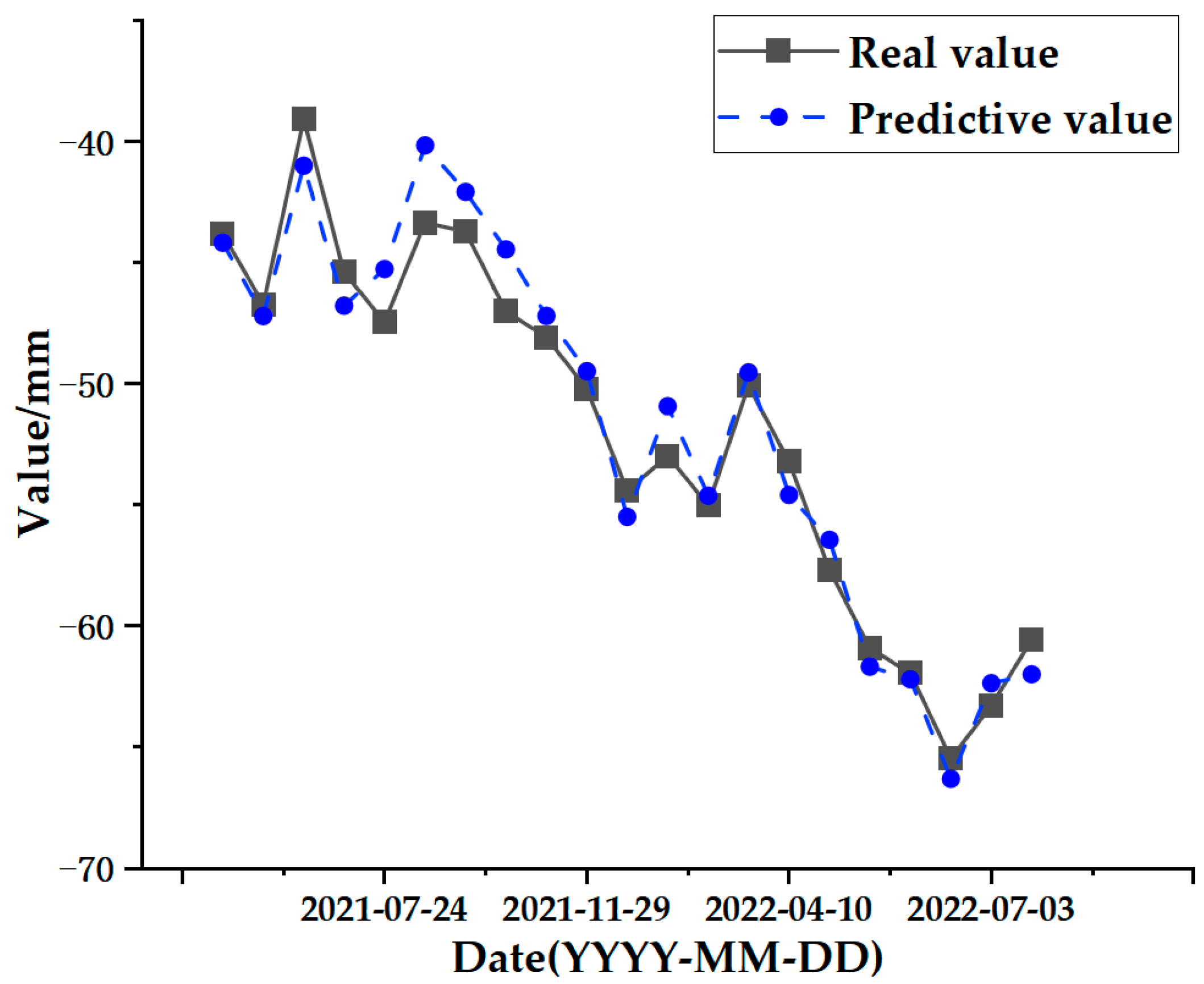
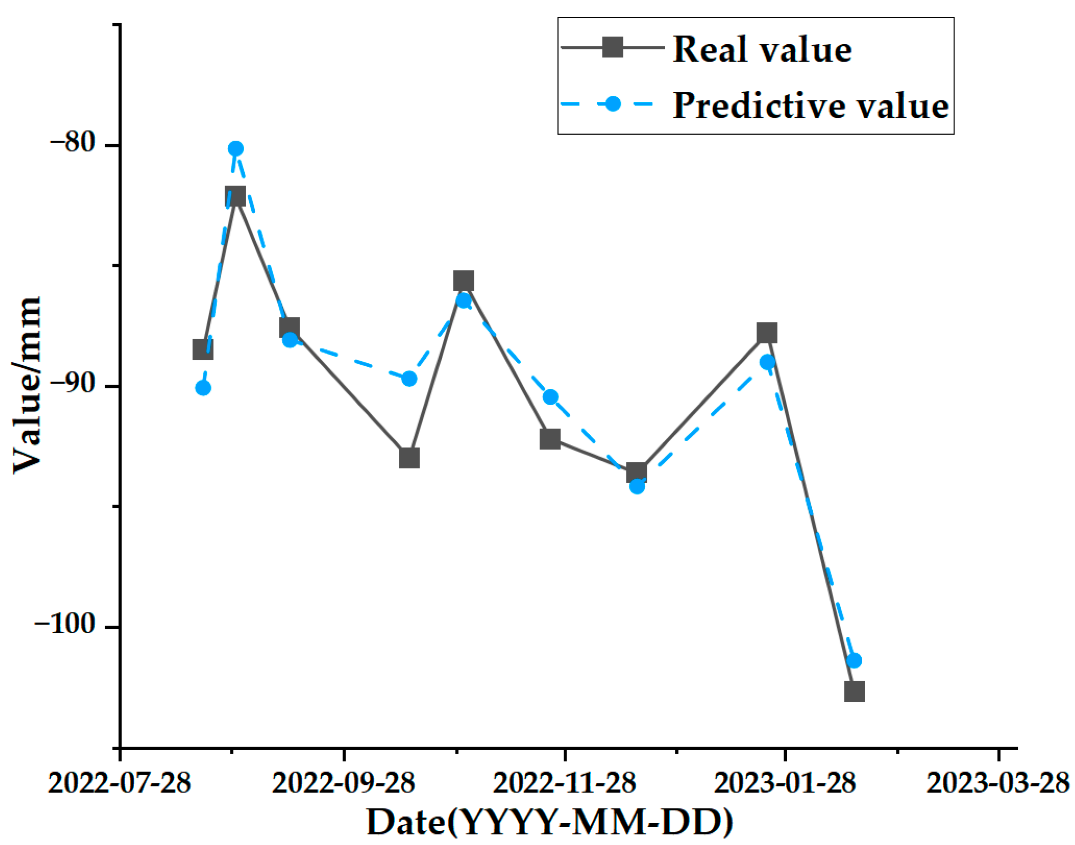
The final output is the data that remains after the SSA-CNN-LSTM model’s prediction to obtain the surface deformation prediction value for the time series.


 ,
, 


