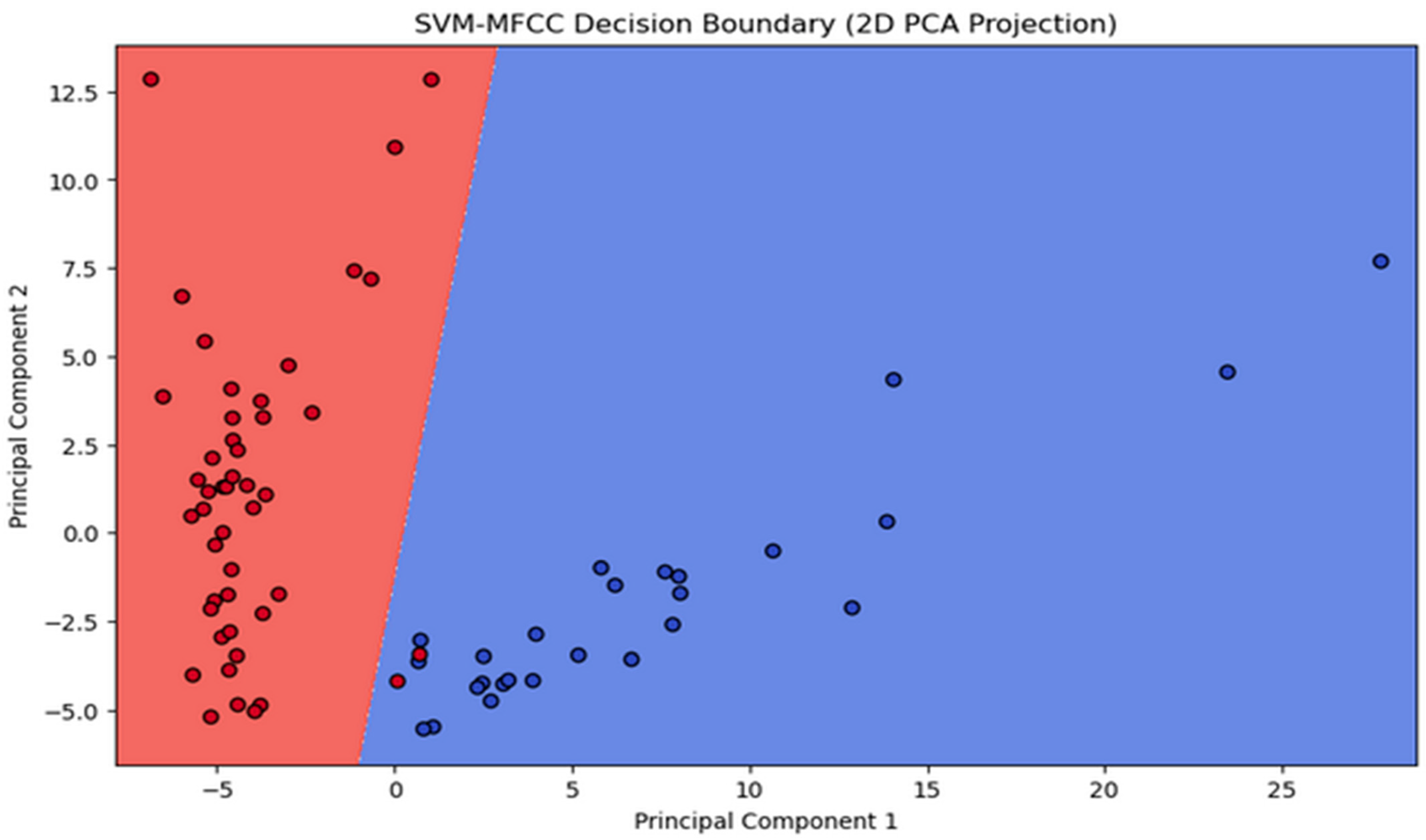
Support Vector Machine (SVM)
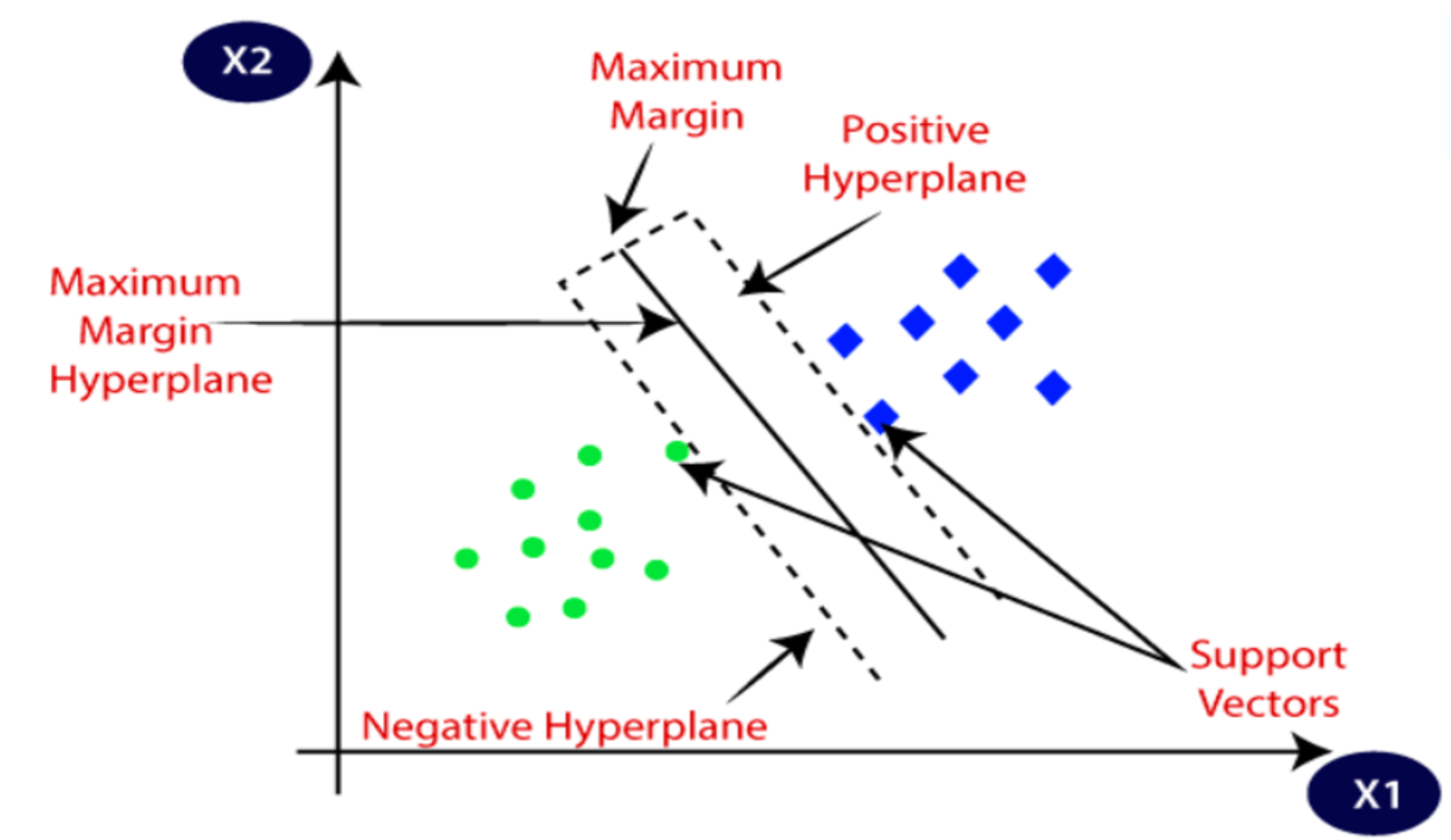
SVM, a binary classifier, distinguishes speakers from impostors via a separation hyperplane. Exploring SVM techniques assesses novel classification methods for speaker identification, enhances comprehension of the challenge, and determines whether SVMs offer insights beyond traditional GMM approaches. SVM utilizes a kernel function to create a binary classifier, with the sequence kernel based on generalized linear discriminants. Notably, it directly expands into the SVM feature space while maintaining computational efficiency and increased accuracy. SVM complements and competes effectively with other methods, including Gaussian mixture models. It seeks the optimal hyperplane that maximizes the margin between data and the separation boundary, resulting in the best generalization performance [
41].
Figure 9 shows the principle of the optimal hyperplane and the optimal margin in SVM modeling.
The discriminant function of the SVM is given by:
where the
are the ideal outputs,
, and
αi > 0. The vectors
are support vectors and are obtained from the training set by an optimization process. The ideal outputs are either 1 or −1, based on the support vector class. The kernel
is constrained to have certain properties (the Mercer condition), so that
can be expressed as:
maps input space in SVM, where a two-class model for speaker identification is trained. The known non-targets comprise the second class, with class 0 assigned to the target speaker’s utterances.
SVM can be represented as a two-class problem: target and nontarget speaker. If ω is a random variable representing the hypothesis, then ω = 1 represents the target being present and ω = 0 represents the target not being present. A score is calculated from a sequence of observations
extracted from the speech input. The scoring function is based on the output of a generalized linear discriminant function of the form
where
is the vector of classifier parameters and
is an expansion of the input space into a vector of scalar functions [
33]:
If the classifier is trained with a mean-squared error training criterion and ideal outputs of 1 for
and 0 for
, then
will approximate the posterior probability
. We can then find the probability of the entire sequence,
as follows:
Taking
on both sides [
33], we obtain the discriminant function:
For classification purposes, we discard
. Using
:
Assuming
:
where the mapping
by is:
In the scoring method, for a sequence of input vectors and a speaker model , we can construct b using (30). For speaker identification, if the score is above a threshold, then we declare the identity claim valid; otherwise, the claim is rejected as an impostor attempt.
Deep Learning-Based Models Architecture
In recent years, deep learning-based models have become the cornerstone for audio classification tasks, enabling the automatic categorization of audio signals into various classes, such as speech recognition, music genre classification, and environmental sound analysis. These models, characterized by their sophisticated architectural design, have demonstrated remarkable performance in handling complex audio data, making them an indispensable tool in various domains including multimedia analysis, content recommendation, and surveillance systems. DNN excels here by leveraging multiple filters during training to extract unique features from input spectrograms. These features improve the representation of active speakers in speech data, autonomously learned and then used for identification by a classifier [
83]. In this section, we explore CNN-LSTM and TDNN architectures as the two main ones that have been employed in this work.
- 1.
Convolutional Long Short-Term Memory Network
CNN, a deep learning model based on convolution, is primarily used for image analysis in machine learning. However, it has shown broad utility in recognizing audio patterns, improving images, processing natural language, and forecasting time series data. The CNN architecture, introduced by Lecun et al. [
84], consists of an input layer, an output layer, and concealed layers, with convolutional layers performing dot product operations between input matrices and convolutional kernels.
A Long Short-Term Memory (LSTM) Network belongs to the category of recurrent neural networks (RNNs), which are essentially neural networks with feedback loops [
85]. RNNs perform well in speech recognition, language modeling, and translation, but they face a key challenge: the vanishing gradient problem. This occurs when the error gradient dwindles or grows explosively during backpropagation, especially across multiple time steps, leading to limited memory capacity, often called ‘
short memory’. LSTM network architecture offers a solution by using a special memory cell to control information flow. This selectively retains or discards data, preventing gradient problems and enabling the learning of long-term dependencies in sequential data.
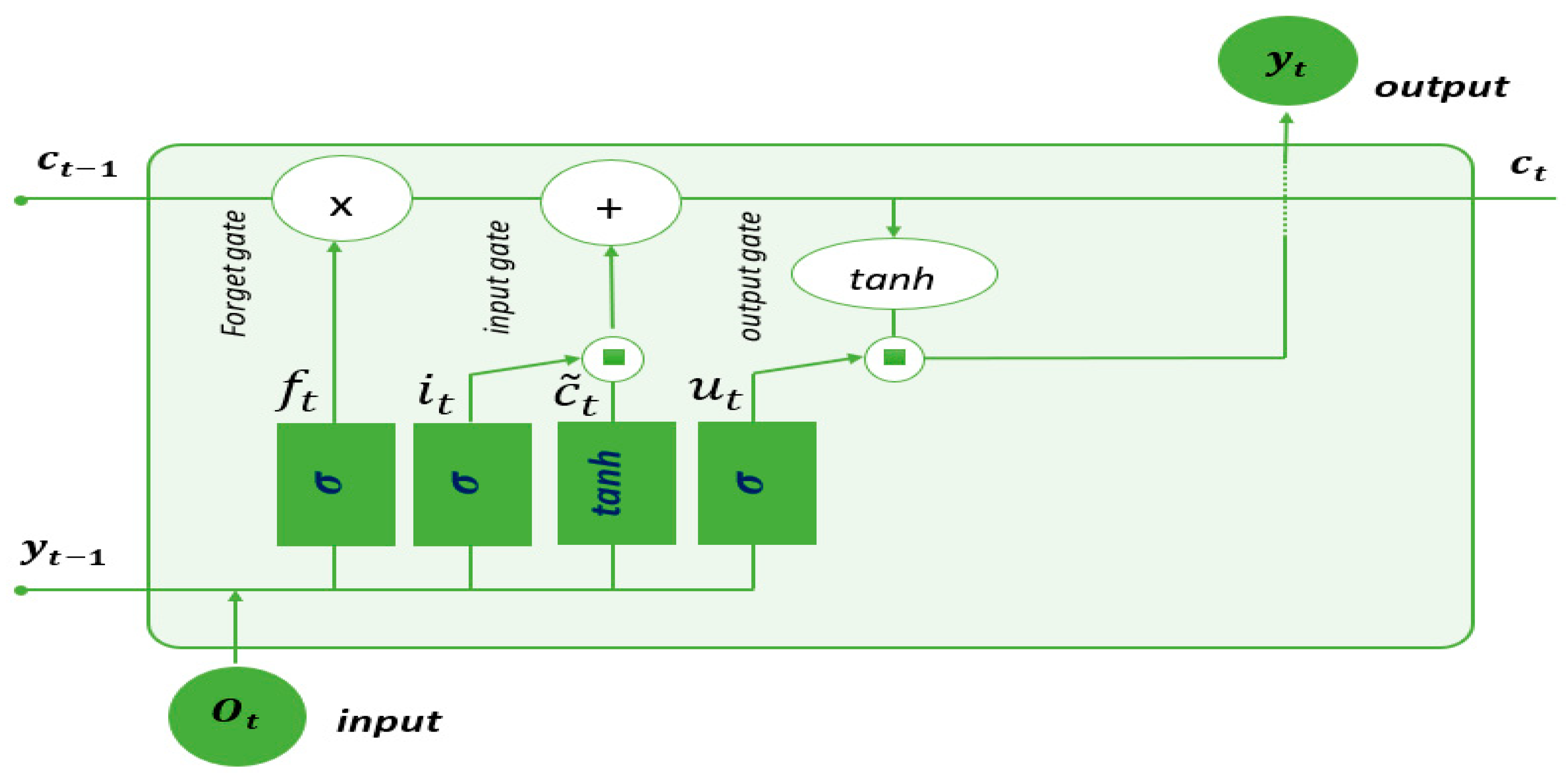
Figure 10 illustrates the architecture of an LSTM cell. Each cell receives two critical inputs: the output sequence produced by the previous LSTM cell and the hidden state value from the previous cell, denoted as
. Inside the cell, there are three gates: the forget gate
, the input gate
, and the output gate
.
Information from the previous hidden state
and information from the current input
are passed through the sigmoid function. The forget gate acts as a filter to forget certain information about the state of the cell. To this end, a term-to-term multiplication is carried out between
and
, which tends to cancel the components of
close to 0. A filtered cell state is then obtained as follows:
where
σ denotes the sigmoid activation function, which is a nonlinear function that maps its input to a value between 0 and 1
is the weight of the forget gate, and
is the bias. The weights and bias values are acquired through the training process of the LSTM.
LSTM employs the input gate for data integration into the memory cell, comprising the input activation gate and the candidate memory cell gate. The input activation gate manages data integration, while the candidate memory cell gate governs data storage within the memory cell.
By considering both the previous hidden state
and the current input node
, the input gate in an LSTM generates two essential vectors: the input vector
and the candidate memory cell vector
. Equation (32) describes the operation of the input activation gate, which involves the weight matrix
and bias vector
. Simultaneously, Equation (33) demonstrates the formation of the candidate memory cell
by applying the hyperbolic tangent activation function (
) to the same set of inputs, utilizing the weight matrix
and bias vector
The input vector and the candidate memory cell vector are merged to update the previous memory cell
, as shown in Equation (34). In this equation, the symbol
⊙ represents element-wise multiplication.
The output gate controls data transfer from the memory cell to the current hidden state, serving as the LSTM’s output. The output gate vector
is computed with this equation:
Subsequently, the current hidden state,
, is derived using following equation:
The new cell state and that of the hidden state are then directed to the next time step. Training sequential neural networks minimizes loss over data sequences using backpropagation through time (BPTT) for temporal gradients. Weight updates are computed mathematically based on loss function L and the learning rate
can be expressed as:
In this paper, the CNN-LSTM architecture utilizes CNN layers to construct a model of an active speaker from input data to enhance the model’s ability to make sequence predictions.
- 2.
Time-delay neural networks (TDNNs)
A Time-Delay Neural Network (TDNN) is a dynamic network designed to capture temporal relationships between events and maintain temporal translation invariance. Initially introduced to enhance modeling of extensive temporal context [
43], TDNN models have found applications in spoken word and online handwriting recognition. TDNN remains a common choice for acoustic modeling in modern speech recognition software such as Kaldi [
84]. Its primary function is to convert acoustic speech signals into sequences of phonetic units, known as ‘phones’. The network takes acoustic feature frames as input and produces output depicting probability distributions for each phonetic unit. The network takes acoustic feature frames as input and produces a probability distribution for a defined set of target language phones. The goal is to classify each frame into the phonetic unit with the highest likelihood. In a single TDNN layer, each input frame is represented as a column vector, symbolizing a time step, with rows representing feature values. A compact weight matrix, often called a kernel or filter, slides over the input signal, performing convolution to generate the output.
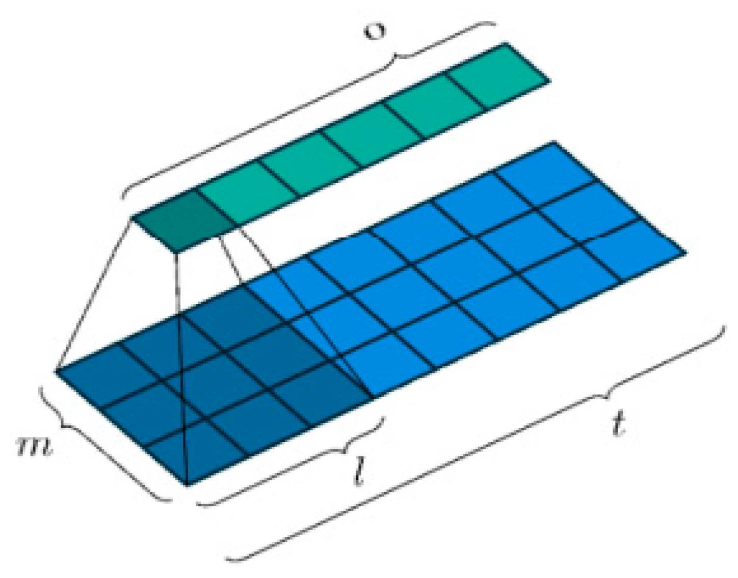
Consider an input vector
in
as a matrix containing m numerical values, such as amplitudes at a specific frequency or the values of acoustic features within a filter bank bin. At each time step t, we will have a matrix of input features
X ∈
where each vector represents one-time step t of our speech signal with a trainable weight matrix
W ∈
, where the kernel maintains a consistent height of
and a width of
, as illustrated in
Figure 11.
The kernel
moves across the input signal with a space of
making s steps in each movement. The area on the input feature map that the kernel encompasses is termed the “receptive field.” Depending on the specific implementation, it is possible that the input may be filled with null values at both ends of height of
and a length of
. The output width
, resulting from the number of times the kernel can fit over the length of the input sequence, can be calculated as follows:
where
represents the floor function.
During each time step t, the TDNN conducts a convolution operation, which involves performing an element-wise multiplication (commonly known as the Hadamard product) between the kernel weights and the input located below it, followed by the summation of these resulting products.
Within the neural network, a trainable bias term b is included (which is not shown in the images above). The outcome is then processed through a non-linear activation function denoted as
(examples of which include sigmoid, rectified linear, or p-norm functions). This process results in the formation of an output
where
represents the entire output vector, achieved by performing this operation across all time steps (depicted as the light green vector in the images). Hence, the concise representation of the scalar output for a single element, denoted as
, at the
-th output step within the set {1,2…, o}, can be expressed as:
where ∗ denotes the convolution operation and
are the inputs in the receptive field. It can also be equivalently given by:
In this equation, the initial summation extends across the height of the acoustic features, while the subsequent summation covers the width of the receptive field or the width of the kernel. It is important to note that the kernel weights are shared across all output steps q. Because the weights of the kernel are shared across the convolutions, the TDNN acquires a representation of the input that remains insensitive to the precise location of a phone within the broader sequence. Additionally, this sharing of weights reduces the quantity of parameters that need to be trained.
Considering that we need to repeat the same convolution operation as before, denoted as , it is important to note that the input vectors have also grown due to the expanded receptive field. In simpler terms, this process involves extracting the receptive field from its input, combining it, and applying the identical convolution operation.
Finally, in the context of employing multiple kernels, represented as H kernels, where each kernel is can be represented as , where each kernel similarly moves across the input. This process results in the generation of a sequence of output vectors, which can be structured into an output matrix Z .
Within a deep neural network architecture, this output can subsequently serve as the initial hidden layer of the network and be employed as input for the subsequent layer of the TDNN.


