
Power-Independent Microwave Photonic Instantaneous Frequency Measurement System


Abstract
1. Introduction
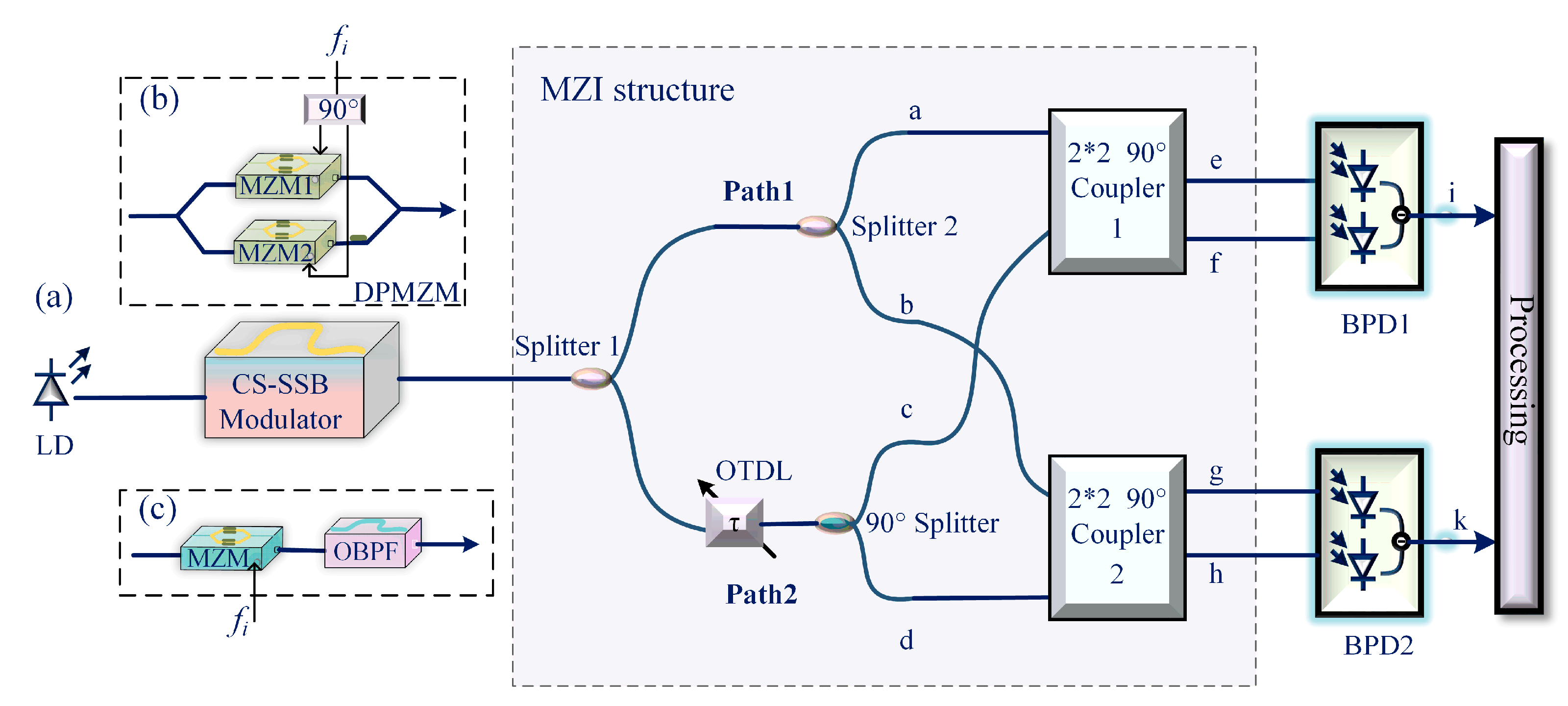
2. Principle
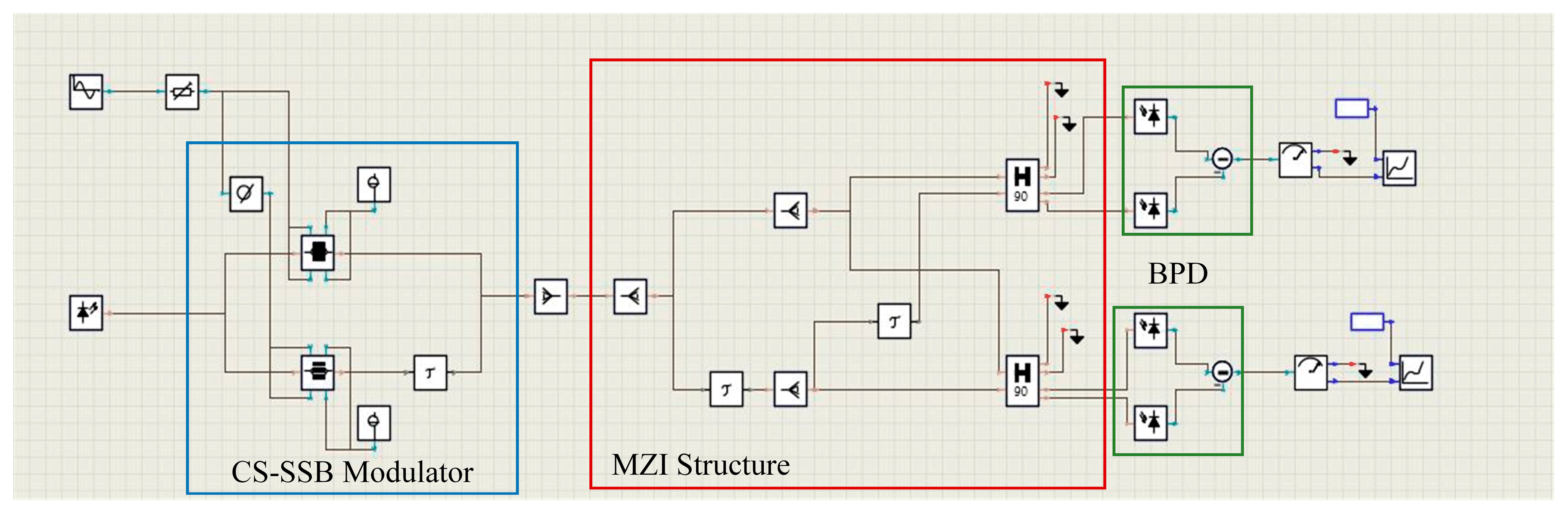
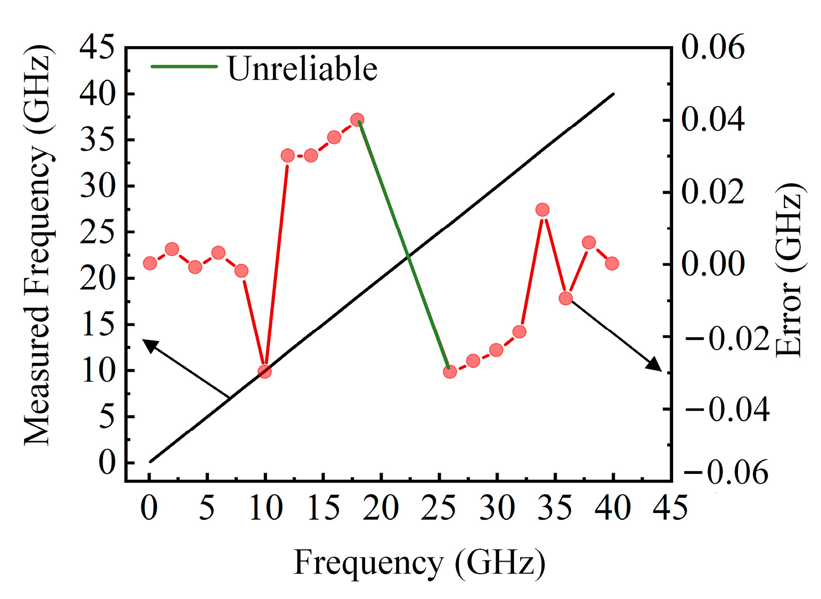
3. Simulation Results
4. Discussion
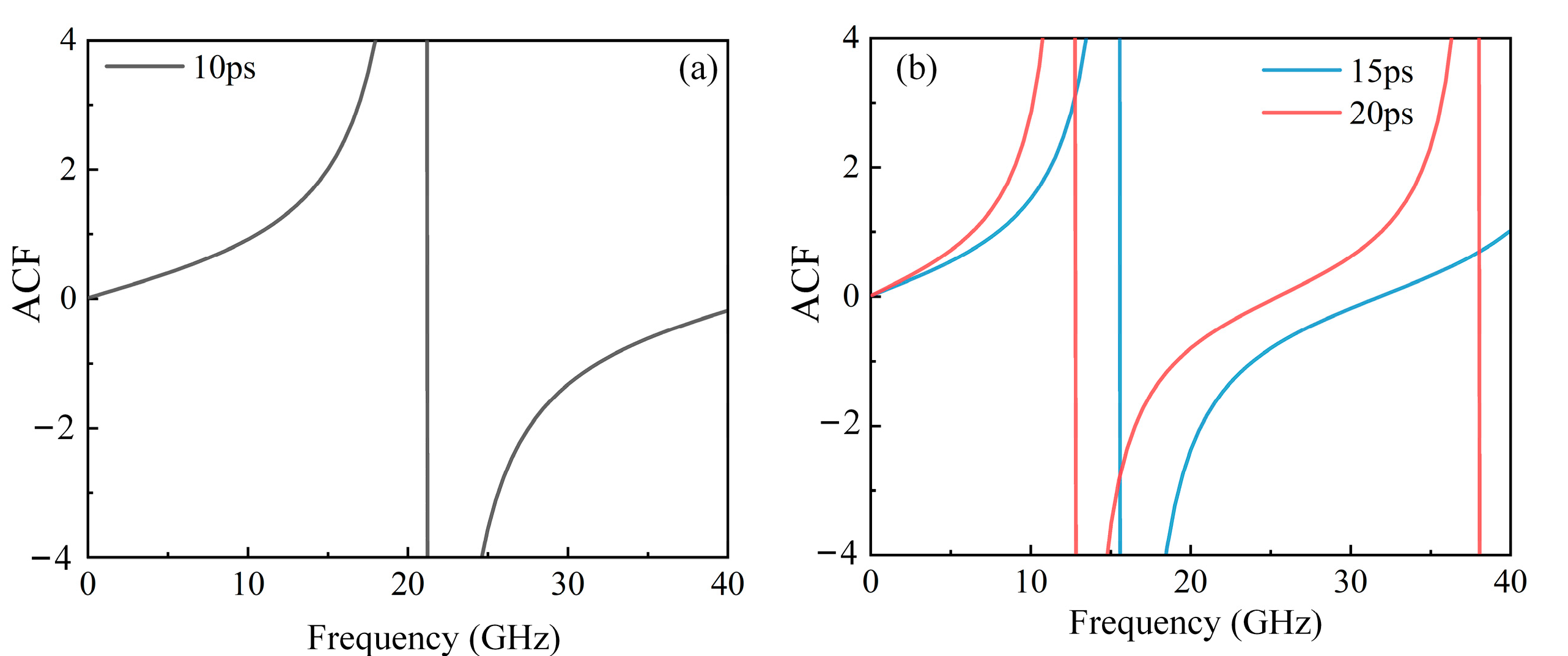
4.1. Discussion on Path Lengths
4.2. Scheme Improvement
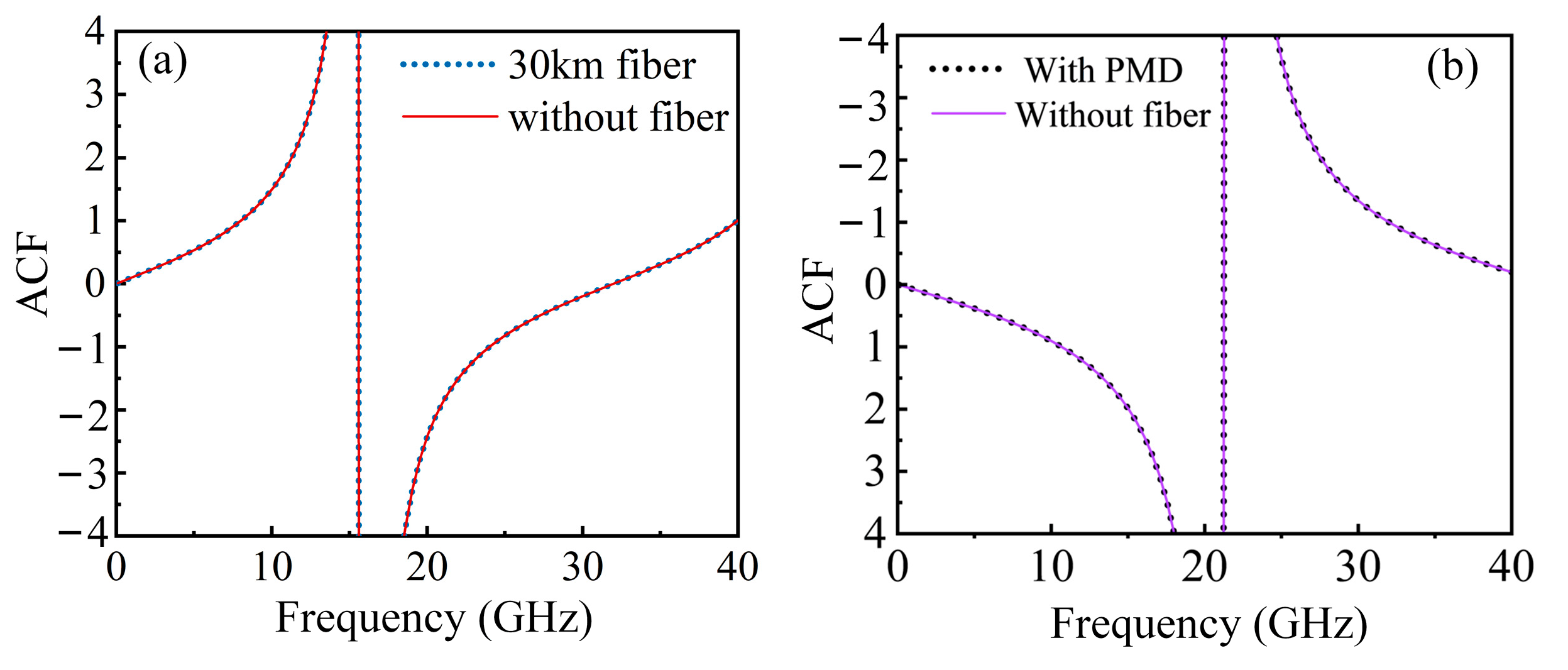
4.3. Long-Distance Measurement
4.4. Carrier-Suppressed Single-Sideband Modulation Experiment
4.5. Scheme Comparison
5. Conclusions
Author Contributions
Funding
Institutional Review Board Statement
Informed Consent Statement
Data Availability Statement
Conflicts of Interest
References
- East, P. Fifty years of instantaneous frequency measurement. IET Radar Sonar Navig. 2012, 6, 112–122. [Google Scholar] [CrossRef]
- Liu, Y.; Sun, J.; Shu, Y.; Wu, L.; Lu, L.; Qi, K.; Che, Y.; Li, L.; Yin, H. High numerical aperture and large focusing efficiency metalens based on multilayer transmitarray elements. Opt. Lasers Eng. 2021, 147, 106734. [Google Scholar] [CrossRef]
- Liu, Y.; Guo, J.; Li, S.; Qi, K.; Li, L.; Yin, H. Low-profile and compact retroreflector enabled by a wide-angle and high-efficiency metalens. Opt. Mater. 2022, 134, 113105. [Google Scholar] [CrossRef]
- Liu, Y.; Zhu, Y.; Wang, Y.; Ren, Z.; Yin, H.; Qi, K.; Sun, J. Monolithically integrated wide field-of-view metalens by angular dispersionless metasurface. Mater. Des. 2024, 240, 112879. [Google Scholar] [CrossRef]
- Pan, S.; Zhang, Y. Microwave Photonic Radars. J. Light. Technol. 2020, 38, 5450–5484. [Google Scholar] [CrossRef]
- Ivanov, A.; Morozov, O.; Sakhabutdinov, A.; Kuznetsov, A.; Nureev, I. Photonic-Assisted Receivers for Instantaneous Microwave Frequency Measurement Based on Discriminators of Resonance Type. Photonics 2022, 9, 754. [Google Scholar] [CrossRef]
- Nguyen, L. Microwave Photonic Technique for Frequency Measurement of Simultaneous Signals. IEEE Photon-Technol. Lett. 2009, 21, 642–644. [Google Scholar] [CrossRef]
- Nguyen, T.; Chan, E.; Minasian, R. Instantaneous high-resolution multiple-frequency measurement system based on frequency-to-time mapping technique. Opt. Lett. 2014, 39, 2419–2422. [Google Scholar] [CrossRef]
- Nguyen, T.; Chan, E.; Minasian, R. Photonic Multiple Frequency Measurement Using a Frequency Shifting Recirculating Delay Line Structure. J. Light. Technol. 2014, 32, 3831–3838. [Google Scholar] [CrossRef]
- Zou, X.; Wang, X.; Zhao, Z.; Wang, B.; Li, X.; Zou, W. Wideband High-Accuracy Microwave Frequency Measurement and Recognition Enabled by Stimulated Brillouin Scattering. Opt. Express 2025, 33, 19627–19640. [Google Scholar] [CrossRef]
- Silva, C.P.D.N.; Espinosa-Espinosa, M.I.; Llamas-Garro, I.; Kim, J.-M.; de Melo, M.T. Review of microwave frequency measurement circuits. J. Electromagn. Waves Appl. 2022, 36, 2055–2087. [Google Scholar] [CrossRef]
- Wang, G.; Meng, Q.; Li, Y.J.; Li, X.; Zhou, Y.; Zhu, Z.; Gao, C.; Li, H.; Zhao, S. Photonic-assisted multiple microwave frequency measurement with improved robustness. Opt. Lett. 2023, 48, 1172–1175. [Google Scholar] [CrossRef] [PubMed]
- Wang, L.; Hao, T.; Guan, M.; Li, G.; Li, M.; Zhu, N.; Li, W. Compact Multi-tone Microwave Photonic Frequency Measurement Based on a Single Modulator and Frequency-to-time Mapping. J. Light. Technol. 2022, 40, 6517–6522. [Google Scholar] [CrossRef]
- Zhou, Y.; Zhang, F.; Pan, S. Instantaneous frequency analysis of broadband LFM signals by photonics-assisted equivalent frequency sampling. Chin. Opt. Lett. 2023, 19, 013901. [Google Scholar] [CrossRef]
- Zou, X.; Pan, W.; Luo, B.; Yan, L. Photonic approach for multiple-frequency-component measurement using spectrally sliced incoherent source. Opt. Lett. 2010, 35, 438–440. [Google Scholar] [CrossRef]
- Li, R.; Chen, H.; Yu, Y.; Chen, M.; Yang, S.; Xie, S. Multiple-frequency measurement based on serial photonic channelization using optical wavelength scanning. Opt. Lett. 2013, 38, 4782–4784. [Google Scholar] [CrossRef]
- Shen, J.; Wu, S.; Li, D.; Liu, J. Microwave multi-frequency measurement based on an optical frequency comb and a photonic channelized receiver. Appl. Opt. 2019, 58, 8101–8107. [Google Scholar] [CrossRef] [PubMed]
- Li, W.; Zhu, N.; Wang, L. Reconfigurable Instantaneous Frequency Measurement System Based on Dual-Parallel Mach–Zehnder Modulator. IEEE Photon-J. 2012, 4, 427–436. [Google Scholar] [CrossRef]
- Zou, X.; Pan, S.; Yao, J. Instantaneous Microwave Frequency Measurement With Improved Measurement Range and Resolution Based on Simultaneous Phase Modulation and Intensity Modulation. J. Light. Technol. 2009, 27, 5314–5320. [Google Scholar]
- Li, Z.; Chi, H.; Zhang, X.; Yao, J. Instantaneous Microwave Frequency Measurement with Improved Measurement Range and Resolution Based on A Polarization Modulator. In Proceedings of the 2010 IEEE International Topical Meeting on Microwave Photonics, Montreal, QC, Canada, 5–9 October 2010. [Google Scholar]
- Yang, C.; Wang, L.; Liu, J. Photonic-Assisted Instantaneous Frequency Measurement System Based on a Scalable Structure. IEEE Photon- J. 2019, 11, 5501411. [Google Scholar] [CrossRef]
- Emami, H.; Ashourian, M. Improved Dynamic Range Microwave Photonic Instantaneous Frequency Measurement Based on Four-Wave Mixing. IEEE Trans. Microw. Theory Tech. 2014, 62, 2462–2470. [Google Scholar] [CrossRef]
- Li, Z.; Wang, C.; Li, M.; Chi, H.; Zhang, X.; Yao, J. Instantaneous Microwave Frequency Measurement Using a Special Fiber Bragg Grating. IEEE Microw. Wirel. Compon. Lett. 2011, 21, 52–54. [Google Scholar] [CrossRef]
- Chen, H.; Huang, C.; Chan, E.H.W. Photonics-Based Instantaneous Microwave Frequency Measurement System with Improved Resolution and Robust Performance. IEEE Photon-J. 2022, 14, 5856008. [Google Scholar] [CrossRef]
- Wang, G.; Li, X.; Meng, Q.; Zhou, Y.; Zhu, Z.; Gao, C.; Li, H.; Zhao, S. Instantaneous Frequency Measurement with Full FSR Range and Optimized Estimation Error. J. Light. Technol. 2022, 40, 6123–6130. [Google Scholar] [CrossRef]
- Chi, H.; Zou, X.; Yao, J. An Approach to the Measurement of Microwave Frequency Based on Optical Power Monitoring. IEEE Photon-Technol. Lett. 2008, 20, 1249–1251. [Google Scholar] [CrossRef]
- Zou, X.; Pan, W.; Luo, B.; Yan, L. Photonic Instantaneous Frequency Measurement Using a Single Laser Source and Two Quadrature Optical Filters. IEEE Photon-Technol. Lett. 2010, 23, 39–41. [Google Scholar] [CrossRef]
- Li, X.; Wen, A.; Li, X.; Mo, Y.; Zhuo, H. Photonic instantaneous frequency measurement using a dense wavelength-division multiplexer. Appl. Opt. 2021, 60, 8286–8290. [Google Scholar] [CrossRef]
- Li, J.; Pei, L.; Ning, T.; Zheng, J.; Li, Y.; He, R. Measurement of Instantaneous Microwave Frequency by Optical Power Monitoring Based on Polarization Interference. J. Light. Technol. 2020, 38, 2285–2291. [Google Scholar] [CrossRef]
- Rabbani, Z.; Ganjali, M.; Hosseini, S.E. Microwave Photonic IFM Receiver with Adjustable Measurement Range Based on a Dual-Output Sagnac Loop. J. Light. Technol. 2024, 42, 106–112. [Google Scholar] [CrossRef]
- Huang, C.; Chan, E.H.W.; Hao, P.; Wang, X. Wideband High-Speed and High-Accuracy Instantaneous Frequency Measurement System. IEEE Photon-J. 2023, 15, 1–8. [Google Scholar] [CrossRef]
- Wang, R.; Fan, Y.; Qin, S.; Tan, J.; Wang, X.; Tan, Q.; Zhai, W.; Gao, Y. Bidirectional colorless WDM-PON RoF system with large spurious free dynamic range. J. Opt. Commun. Netw. 2022, 14, 389–397. [Google Scholar] [CrossRef]


| Device | LD | DPMZM | ODTL | 90° Coupler | BPD |
|---|---|---|---|---|---|
| Reference devices | Feibo Optoelectronic (Shanghai, China) TLS-M-C-16-P-FA | Fujitsu (Tokyo, Japan) FTM7961EZ | Ziguan(Sichuan, China), ODTL | Kylia (Paris, France) COH24 | Discovery Semiconductors (New Jersey, USA) DSC740 |
| Device website | www.fiber-photonics.com | www.fujitsu.com | www.zg-photonics.com | www.bonphot.com | www.discsemi.com |
| Main parameters | Center wavelength: 1527–1668 nm Power: 16 dBm RIN: −155 dBc/Hz | Half-wave voltage: 3.85 V@10 GHz 4.3 V@20 GHz 4.67 V@30 GHz 4.94 V@40 GHz; Insertion loss: 8 dB | Delay range: 0–700 ps Insertion loss: 0.8 dB | Insertion loss: 1 dB Amplitude/phase error: 0.5 dB/<5° | Responsivity: 0.6 A/W; Amplitude/phase error: 0.5 dB/3° |
| Method | Bandwidth (GHz) | IFM Error Within | Tunable Power |
|---|---|---|---|
| [19] | 2–19 | ±0.2 GHz | Not mentioned |
| [20] | 0.5–40 | ±0.5 GHz | Not mentioned |
| [21] | 1–20 | ±0.1 GHz | Not mentioned |
| [22] | 0.04–40 | 0.1 GHz (0.35%) | 51 dB |
| [23] | 1–10 | ±0.2 GHz | Not mentioned |
| [24] | 8–18 | ±0.15 GHz | Not mentioned |
| [25] | 7.5–20 | 0.1 GHz | Not mentioned |
| [26] | 5–20 | 5% | Not mentioned |
| [27] | 20–36 | ±0.4 GHz | Not mentioned |
| [28] | 1–40 | 0.2% | Not mentioned |
| [29] | 4.4–8.7 | ±0.2 GHz | Not mentioned |
| [30] | 0–14 | 0.075 GHz | Not mentioned |
| This work | Over 30 | −0.03–0.04 GHz (0.3%) | Over 30 dB |
Disclaimer/Publisher’s Note: The statements, opinions and data contained in all publications are solely those of the individual author(s) and contributor(s) and not of MDPI and/or the editor(s). MDPI and/or the editor(s) disclaim responsibility for any injury to people or property resulting from any ideas, methods, instructions or products referred to in the content. |
© 2025 by the authors. Licensee MDPI, Basel, Switzerland. This article is an open access article distributed under the terms and conditions of the Creative Commons Attribution (CC BY) license (https://creativecommons.org/licenses/by/4.0/).
Share and Cite
Wang, R.; Li, Y. Power-Independent Microwave Photonic Instantaneous Frequency Measurement System. Sensors 2025, 25, 4382. https://doi.org/10.3390/s25144382
Wang R, Li Y. Power-Independent Microwave Photonic Instantaneous Frequency Measurement System. Sensors. 2025; 25(14):4382. https://doi.org/10.3390/s25144382
Chicago/Turabian StyleWang, Ruiqiong, and Yongjun Li. 2025. "Power-Independent Microwave Photonic Instantaneous Frequency Measurement System" Sensors 25, no. 14: 4382. https://doi.org/10.3390/s25144382
APA StyleWang, R., & Li, Y. (2025). Power-Independent Microwave Photonic Instantaneous Frequency Measurement System. Sensors, 25(14), 4382. https://doi.org/10.3390/s25144382