

Structural Dynamics Analysis of a Large Aperture Space Telescope Based on the Linear State Space Method

 , , and
Abstract
1. Introduction
2. Linear State Space Representation
- (a)
- Link system outputs to system states and external inputs;
- (b)
- Establish a dynamic time-domain model of the system to realize the internal decoupling of the model;
- (c)
- The short length of the data allows for efficient computation of the problem.
2.1. General Form of a State Space Equation
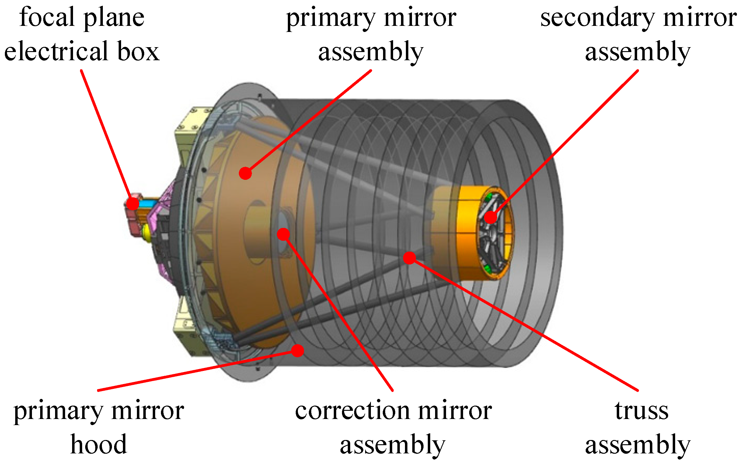
2.2. State Space Model of Optical Remote Sensing Camera
3. Balanced Reduction Method
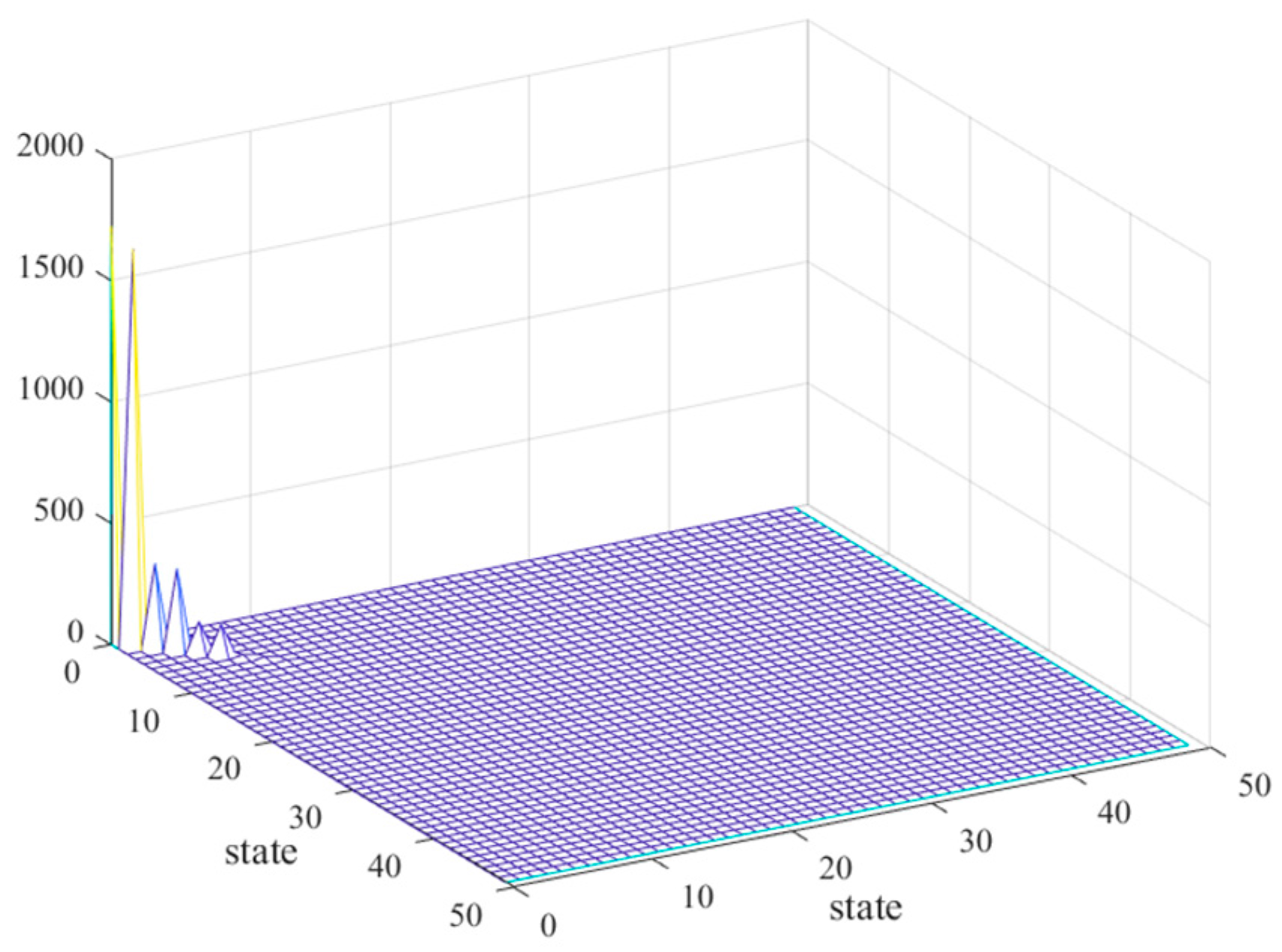
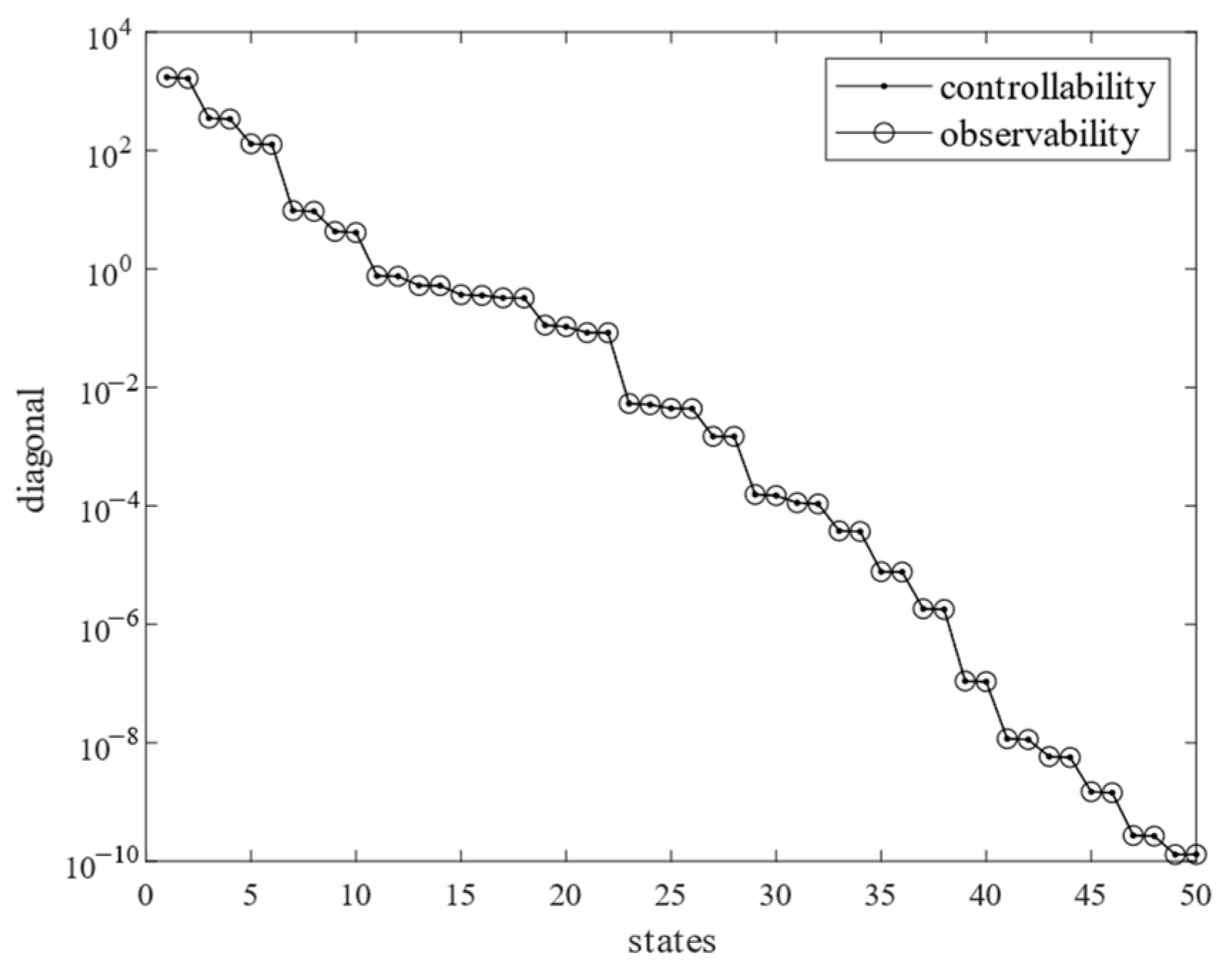
3.1. Controllability and Observability
3.2. Balance Reduction
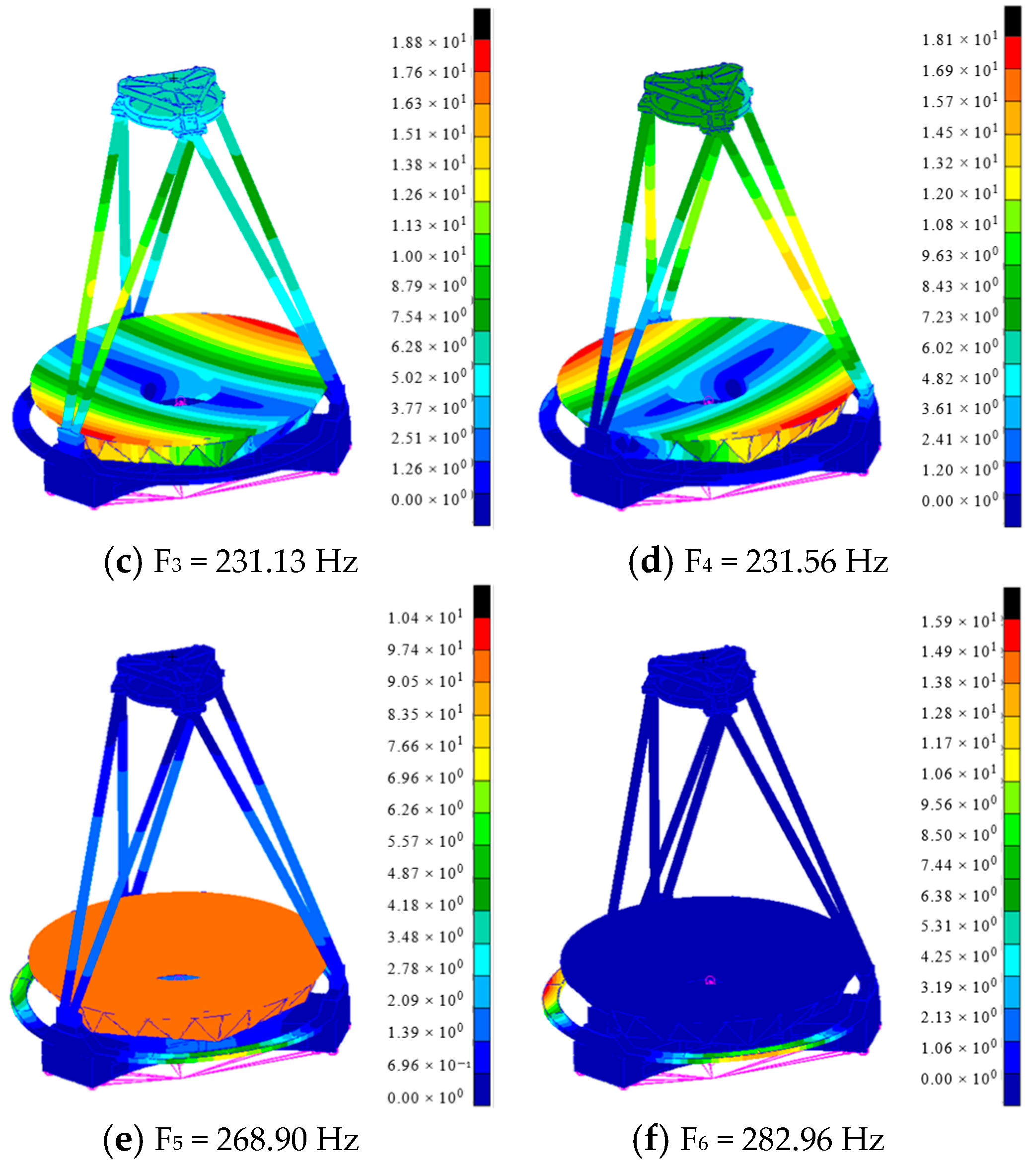
4. Simulation Analysis and Test
4.1. Modal Analysis
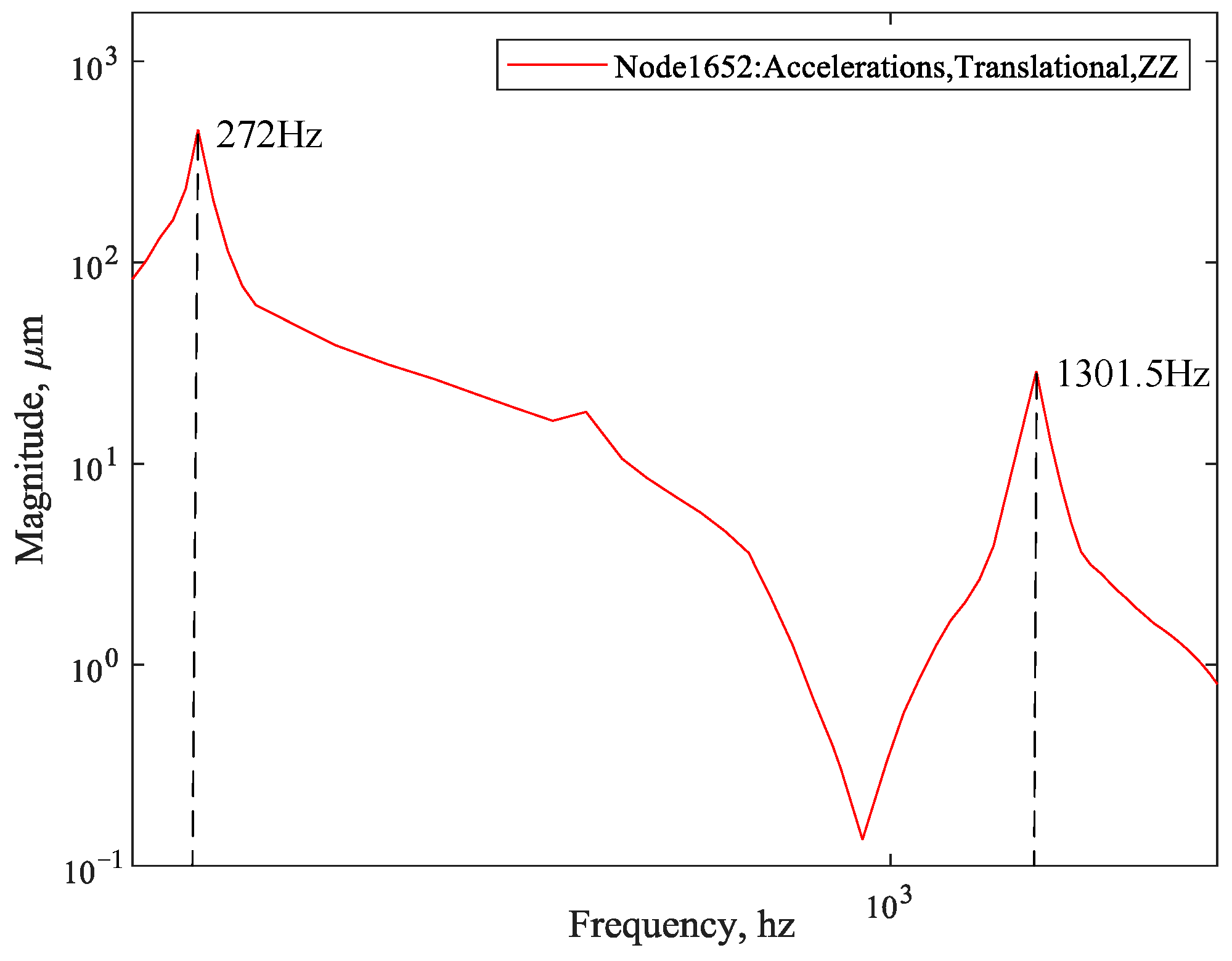
4.2. Frequency Response Analysis with Finite Element Method
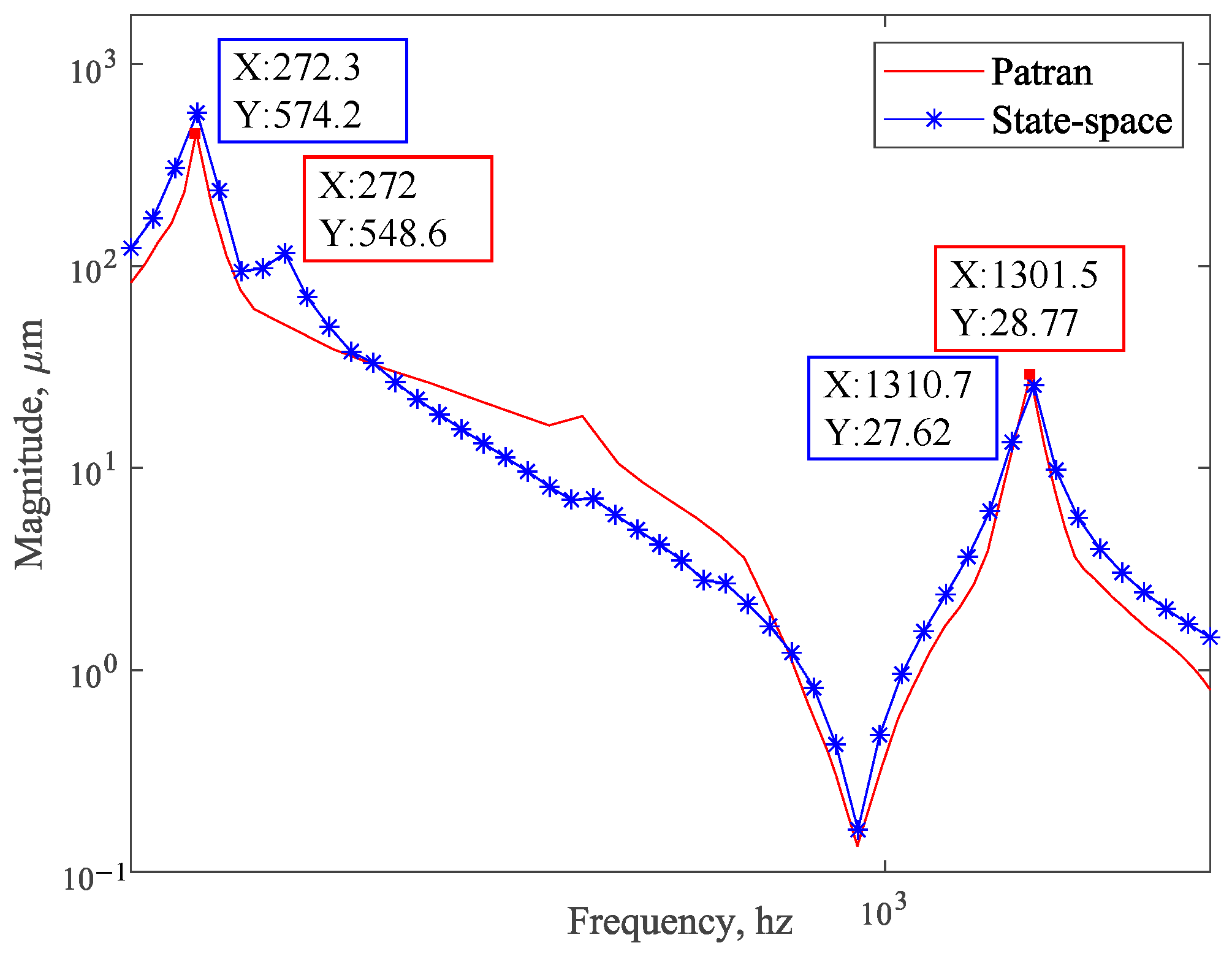
4.3. Frequency Response Analysis with State Space Method
- (1)
- Data acquisition. Perform modal analysis on the finite element model of the whole camera; extract the natural frequency of the appropriate order modal data from the obtained result file; extract the eigenvalues of the system, as shown in Table 2; extract the node displacements of the excitation input point and the response output point, and generate the modal matrix (take the Z-direction displacement as an example, Equation (26)); and determine the frequency range based on the results of the modal analysis.
- (2)
- State space model establishment. Read the data file, establish the state space model of the camera, and plot the frequency transfer characteristic curve.
- (3)
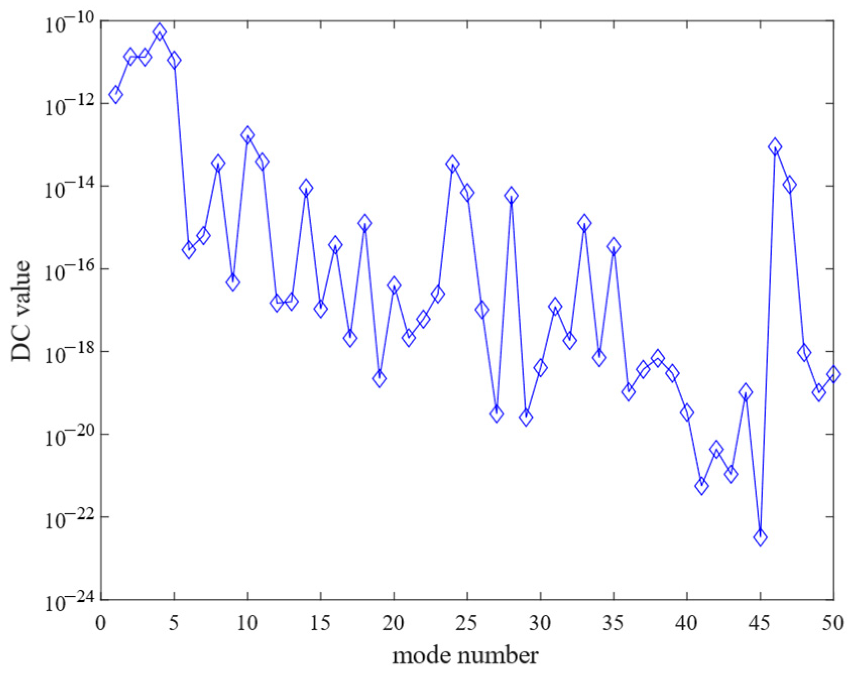
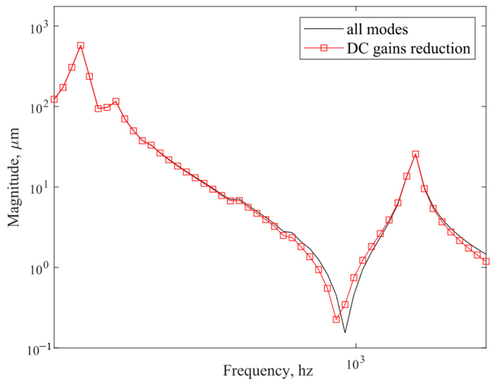
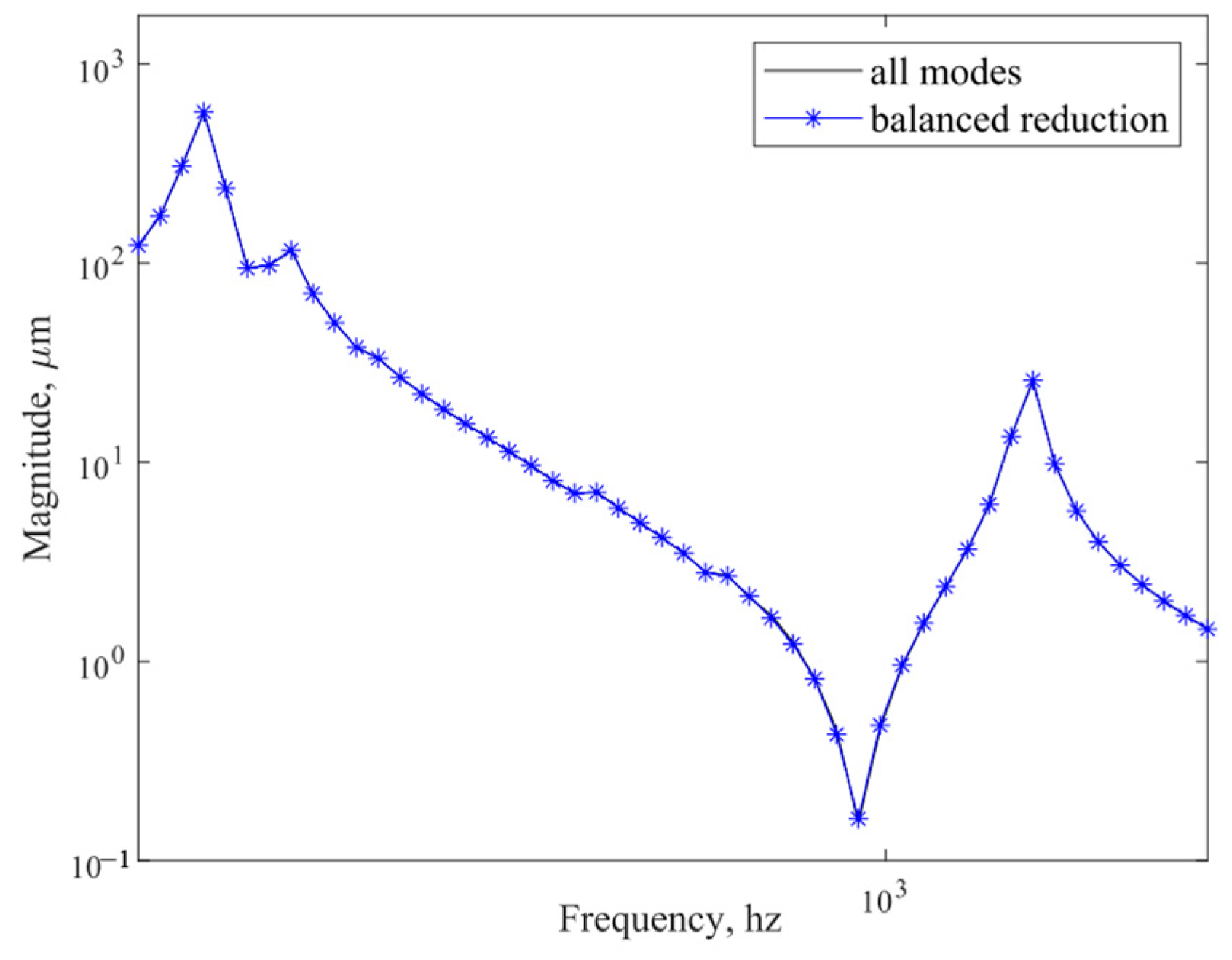
- Modal reduction. Use Equations (9) and (12) to solve the controllability and observability matrices for each non-rigid body mode, and then, use the transformation matrix T to make the diagonal terms of the controllability and observability matrices equal. Sort the matrix diagonal entries from largest to smallest. Modes with non-zero diagonal entries are retained, modes with zero diagonal entries are reduced, and the state space model is regenerated from the retained modes to obtain the modal reduced system model.
- (4)
- Modal reduction results. The frequency response of the simplified system model is calculated to obtain the frequency transfer characteristic curves of nodes 915,737–1652.
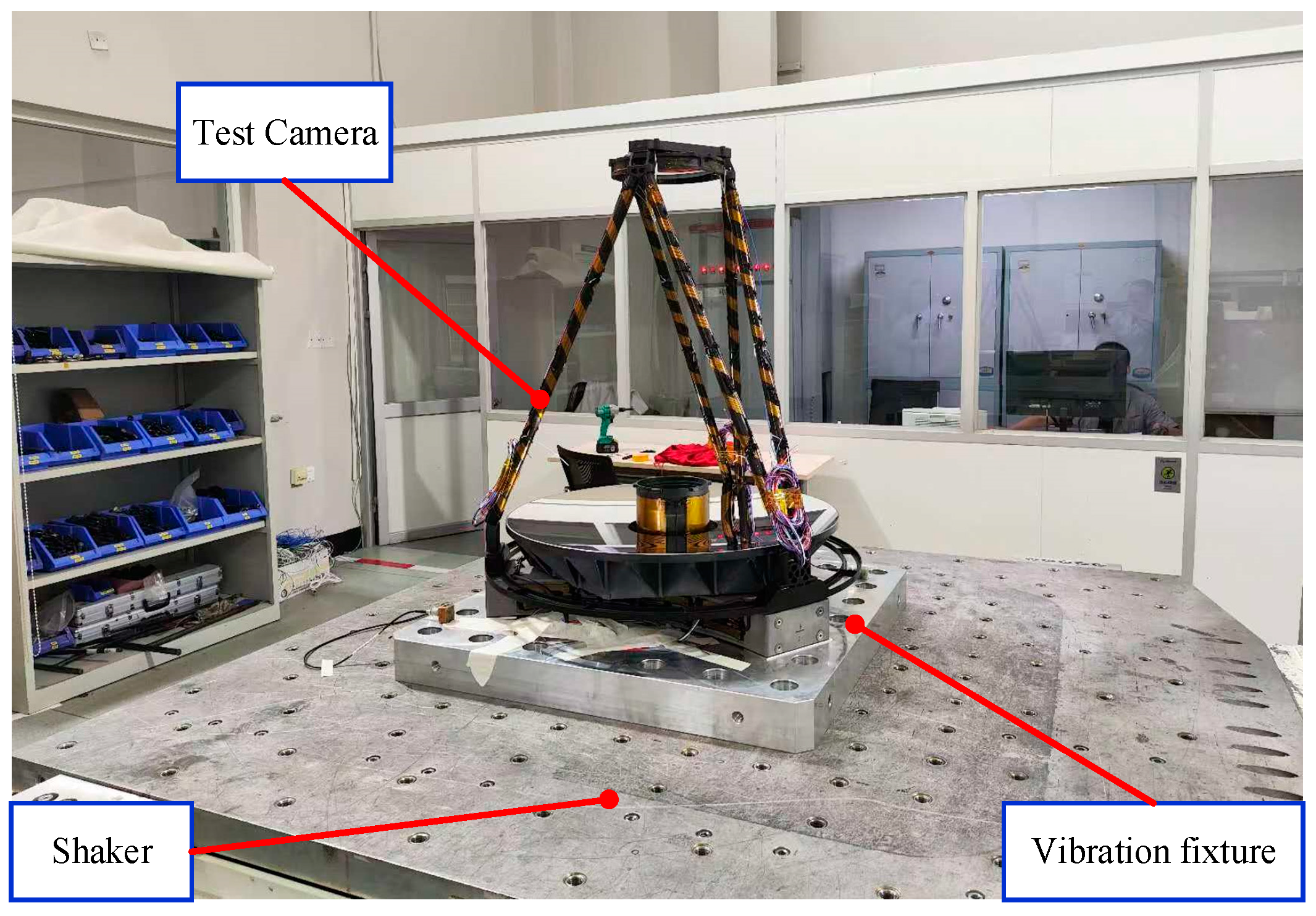
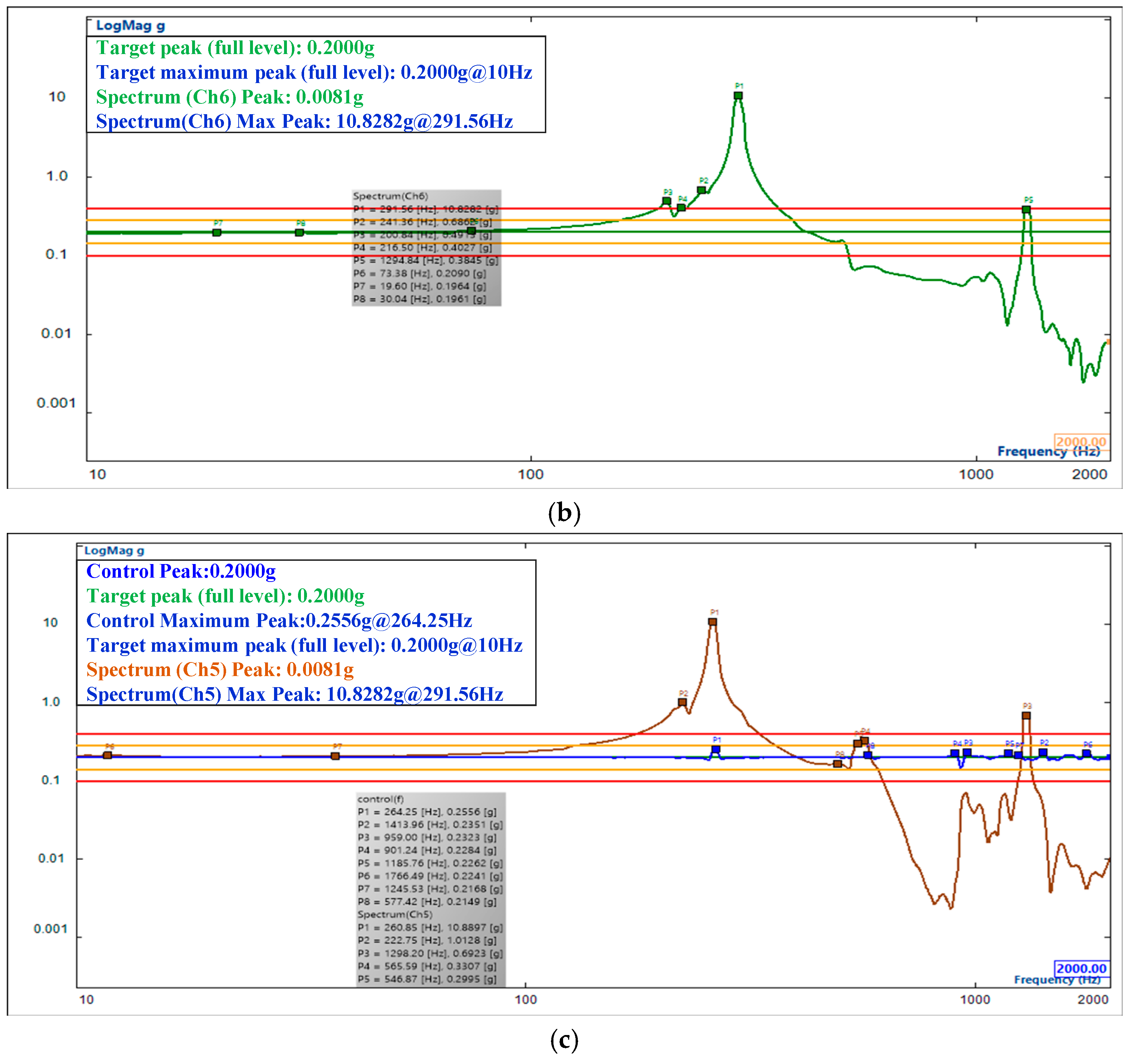
4.4. Dynamic Vibration Test of the Whole Machine
5. Discussion
6. Conclusions
Author Contributions
Funding
Institutional Review Board Statement
Informed Consent Statement
Data Availability Statement
Conflicts of Interest
References
- Zheng, G. Structural Dynamics Sequel: Application in Aircraft Design, 1st ed.; Science Press: Beijing, China, 2016; pp. 406–410. [Google Scholar]
- Ma, B.; Zong, Y.; Li, Z.; Li, Q.; Zhang, D.; Li, Y. Status and prospect of opto-mechanical integration analysis of micro-vibration in aerospace optical cameras. Opt. Precis. Eng. 2023, 31, 822–838. [Google Scholar] [CrossRef]
- Li, L.; Wang, D.; Xu, J.; Tan, L.; Yang, H. Influence of micro-vibration of flywheel components on optical axis of high resolution optical satellite. Opt. Precis. Eng. 2016, 24, 2515–2522. [Google Scholar]
- Li, Z.; Chen, X.; Wang, S.; Jin, G. Optimal design of a Φ760 mm lightweight SiC mirror and the flexural mount for a space telescope. Rev. Sci. Instrum. 2017, 88, 125107. [Google Scholar] [CrossRef] [PubMed]
- Xu, G.; Zhang, B.; Wang, J.; Sun, G.; Gou, Z. Line of Sight Stabilization Validation of Space Optical Telescope Based on Integrated Modeling Method. Spacecr. Eng. 2019, 28, 39–45. [Google Scholar]
- Tang, Y.; Liu, X.; Cai, G.; Liu, X. Active vibration control of a large space telescope truss based on unilateral saturated cable actuators. Acta Mech. Sin. 2022, 38, 522040. [Google Scholar] [CrossRef]
- Yoo, J.; Han, J.Y.; Kim, H.K.; Choi, S.; Lee, W.K. Thermal Analysis and Control Design for Space Optical Telescope ROKITS. Int. J. Aeronaut. Space Sci. 2024, 25, 1554–1562. [Google Scholar] [CrossRef]
- Yu, D.Y.; Lian, M.L.; Zhou, F.; Bai, S.; Lu, Z. Influence of micro-vibration on the image quality of a GEO remote sensor. Sci. Sin. Inform. 2019, 49, 74–86. [Google Scholar] [CrossRef]
- Zhou, X.; Liu, H.; Li, Y.; Ma, M.; Liu, Q.; Lin, J. Analysis of the influence of vibrations on the imaging quality of an integrated TDICCD aerial camera. Opt. Express 2021, 29, 18108–18121. [Google Scholar] [CrossRef] [PubMed]
- Tian, Q.; Sun, H.; Yu, Z. Model order reduction of thermal-dynamic coupled flexible multibody system with multiple varying parameters. Appl. Math. Model 2024, 136, 115634. [Google Scholar] [CrossRef]
- Haber, A.; Draganov, J.E.; Heesh, K.; Tesch, J.; Krainak, M. Modeling and system identification of transient STOP models of optical systems. Opt. Express 2020, 28, 39250. [Google Scholar] [CrossRef] [PubMed]
- Song, X.; Liang, P.; Zhang, S.; Pang, Y.; Gong, Z.; Yang, K.; Zhang, J.; Yuan, Z. A modeling method for the opto-mechanical coupling problems of photoelectric detection and tracking systems in dynamics process. Struct. Multidiscip. Optim. 2024, 67, 170. [Google Scholar] [CrossRef]
- Hahn, L.; Eberhard, P. Transient dynamical-thermal-optical system modeling and simulation. J. Eur. Opt. Soc. Rapid Publ. 2021, 17, 5. [Google Scholar] [CrossRef]
- Jiang, G.; Zhou, K.; Li, Z.; Yan, J. Bearing Dynamics Modeling Based on the Virtual State-Space and Hammerstein–Wiener Model. Sensors 2024, 24, 5410. [Google Scholar] [CrossRef] [PubMed]
- Liu, R.; Li, Z.; Xu, W.; Yang, X.; Zhang, D.; Yao, Z.; Yang, K. Dynamic Analysis and Experiment of a Space Mirror Based on a Linear State Space Expression. Appl. Sci. 2021, 11, 5379. [Google Scholar] [CrossRef]
- Košarac, A.; Zeljković, M.; Mlađenović, C.; Živković, A.; Prodanović, S. State Space Modeling from FEM Model Using Balanced Reduction. In Proceedings of the 5th International Conference Industrial Engineering and Environmental Protection–IIZS, Zrenjanin, Serbia, 15–16 October 2015. [Google Scholar]
- Ding, Z.; Li, L.; Hu, Y. A modified precise integration method for transient dynamic analysis in structural systems with multiple damping models. Mech. Syst. Signal Process. 2018, 98, 613–633. [Google Scholar] [CrossRef]
- Haber, A.; Draganov, J.E.; Heesh, K.; Cadena, J.; Krainak, M. Modeling, experimental validation, and model order reduction of mirror thermal dynamics. Opt. Express 2021, 29, 24508–24524. [Google Scholar] [CrossRef] [PubMed]
- Preumont, A. Vibration Control of Active Structures: An Introduction; Springer: New York, NY, USA, 2018; pp. 289–308. [Google Scholar]
- Hatch, M.R. Vibration Simulation Using MATLAB and ANSYS; Chapman & Hall/CRC: Boca Raton, FL, USA, 2000; pp. 542–575. [Google Scholar]
- Gawronski, W.K. Advanced Structural Dynamics and Active Control of Structures; Springer: New York, NY, USA, 2004; pp. 65–165. [Google Scholar]
- Andersen, T.; Enmark, A. Integrated Modeling of Telescopes; Springer: New York, NY, USA, 2011; pp. 253–308. [Google Scholar]


| Order | F1 | F2 | F3 | F4 | F5 | F6 |
|---|---|---|---|---|---|---|
| Frequency | 222.28 | 223.89 | 231.13 | 231.56 | 268.90 | 282.96 |
| Mode | Frequency | Eigenvalue |
|---|---|---|
| 1 | 2.222793 × 10² | 1.950553 × 10⁶ |
| 2 | 2.238885 × 10² | 1.978898 × 10⁶ |
| 3 | 2.311281 × 10² | 2.108945 × 10⁶ |
| 4 | 2.315579 × 10² | 2.116795 × 10⁶ |
| 5 | 2.688967 × 10² | 2.854503 × 10⁶ |
| 6 | 2.829597 × 10² | 3.160886 × 10⁶ |
| 7 | 2.832125 × 10² | 3.166536 × 10⁶ |
| 8 | 2.841080 × 10² | 3.186594 × 10⁶ |
| 9 | 2.873277 × 10² | 3.259227 × 10⁶ |
| 10 | 3.274861 × 10² | 4.233947 × 10⁶ |
| Tool | MSC Patran/Nastran | State Space Model |
|---|---|---|
| Analytical process | 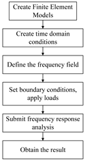 | 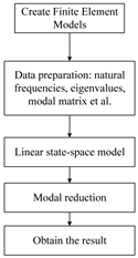 |
| Consuming time | 20 min | 20.036 s |
| X Direction | Y Direction | Z Direction | ||||
|---|---|---|---|---|---|---|
| Fundamental Frequency | Relative Error | Fundamental Frequency | Relative Error | Fundamental Frequency | Relative Error | |
| FEA simulation | 308 Hz | 5.37% | 308 Hz | 5.64% | 272 Hz | 4.27% |
| Test | 292.31 Hz | 291.56 Hz | 260.85 Hz | |||
Disclaimer/Publisher’s Note: The statements, opinions and data contained in all publications are solely those of the individual author(s) and contributor(s) and not of MDPI and/or the editor(s). MDPI and/or the editor(s) disclaim responsibility for any injury to people or property resulting from any ideas, methods, instructions or products referred to in the content. |
© 2025 by the authors. Licensee MDPI, Basel, Switzerland. This article is an open access article distributed under the terms and conditions of the Creative Commons Attribution (CC BY) license (https://creativecommons.org/licenses/by/4.0/).
Share and Cite
Ma, B.; Li, Z.; Li, L.; Li, Y.; Peng, Y.; Ren, S.; Li, Q.; Xu, J. Structural Dynamics Analysis of a Large Aperture Space Telescope Based on the Linear State Space Method. Sensors 2025, 25, 2476. https://doi.org/10.3390/s25082476
Ma B, Li Z, Li L, Li Y, Peng Y, Ren S, Li Q, Xu J. Structural Dynamics Analysis of a Large Aperture Space Telescope Based on the Linear State Space Method. Sensors. 2025; 25(8):2476. https://doi.org/10.3390/s25082476
Chicago/Turabian StyleMa, Bin, Zongxuan Li, Lin Li, Yunfeng Li, Youhan Peng, Shuhui Ren, Qingya Li, and Jiakun Xu. 2025. "Structural Dynamics Analysis of a Large Aperture Space Telescope Based on the Linear State Space Method" Sensors 25, no. 8: 2476. https://doi.org/10.3390/s25082476
APA StyleMa, B., Li, Z., Li, L., Li, Y., Peng, Y., Ren, S., Li, Q., & Xu, J. (2025). Structural Dynamics Analysis of a Large Aperture Space Telescope Based on the Linear State Space Method. Sensors, 25(8), 2476. https://doi.org/10.3390/s25082476