Abstract
This paper is concerned with sensor data transmission strategy. The main focus of the paper is how to reduce the number of sensor data transmission while maintaining the difference between the estimated sensor value and the real sensor value. The proposed method could be used in sensor networks and networked control systems, where number of transmission should be minimal. A linear predictor is used to predict sensor values and sensor data are transmitted if the difference between the predicted sensor value and the real sensor value exceeds the specified limit. An analytic upper bound of the mean rate of messages is provided. Through simulation, it is shown that the number of transmission could be significantly reduced compared with the periodic sampling and the conventional send-on-delta method.
1. Introduction
Periodic sampling of sensor data is used in many applications since it is easy to implement and there are well-established system theory for periodically sampled signals [1].
However, there are applications, where periodic sampling is not desirable. In networked control systems [2, 3], several sensors are connected through a serial network. Sometimes only limited bandwidth is allowed for sensor data transmission; for example, the network physical bandwidth may be limited or most of a network traffic could be used by other control/monitoring traffic. In this case, periodic sampling is not suitable since transmission rate of the period sampling is generally high.
Another example is a wireless sensor networks [4], where a sensor node is battery-powered and the battery power should be saved for longer operation time. As experimented in [5], wireless transmission consumes significantly more power compared with internal computation. Thus to reduce the battery consumption, a sampling method, which requires less transmission, is desirable.
As a transmission frequency reducing method, an event-driven sampling is a gaining popularity. In an event-driven sampling, a sampling is taken if an event happens: for example, an event could be a sensor value change exceeding the specified limit. This event-driven sampling has many names: magnitude-driven sampling [6] a deadzone method [7], a send-on-delta method [8, 9] and Lebesque sampling [10].
Despite many names, the basic principle is the same. If we explain in the framework of a networked monitoring system, a sensor data is transmitted when the difference between last transmitted value and the current value is larger than the specified limit. When a signal change is relatively small, number of sensor data transmission is significantly less than that of the periodic sampling method. This event-driven sampling is used in many intelligent sensors and also a standard feature in Lon Network [11], which is mainly used in the Building Automation.
In this paper, we propose a transmission algorithm for intelligent sensors, which further reduces the number of transmission. In the algorithm, a sensor value is transmitted if difference between the current value and the predicted value is larger than the specified limit. The predicted value is computed using the past values. In fact, the send-on-delta method could be considered as a special case of the proposed algorithm in the sense that the predicted value is just the last transmitted value. In the send-on-delta method, the number of transmission is small when the signal does not change; that is when the first derivative is almost constant.
In the proposed algorithm, the number of transmission is reduced when the higher order (2nd and 3rd) derivative is almost constant. It is shown that the proposed algorithm reduces the number of transmission compared with the conventional send-on-delta methods.
The paper is organized as follows. In Section 2, we propose a new algorithm which combines send-on-delta concept with a linear predictor. In Section 3, we investigate the mean rate of messages for the proposed algorithm. We provide an explicit upper bound for the mean rate of messages. In Section 4, simulations are done for four signals so that we can compare the periodic sampling method, the send-on-delta method, and the proposed method. Conclusion is given in Section 5.
2. Send-on-delta transmission with a linear predictor
The conventional send-on-delta method [8, 9] is illustrated in Fig. 1. The sensor value is transmitted when the difference between the current value x(t) and the last transmitted value xlast(t) is larger than specified δ. In this method, the error (x(t) − xlast(t)) in the monitoring station (where sensor data are received) is always smaller than δ assuming there is no delay and packet loss during transmission.
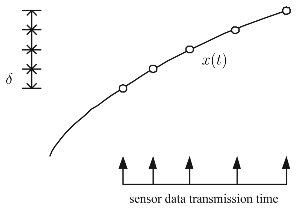
Figure 1.
Conventional send-on-delta transmission
We propose a new algorithm (see Fig. 2), which combines the send-on-delta concept and a linear predictor. After the sensor value transmission, a linear predictor computes the future sensor value ̂ based on the past values. If the difference between the current value and the predicted value is larger than δ, the sensor value is transmitted. Note that ̂ is computed both in the sensor node and monitoring station. Also note that the error (x(t) − ̂(t)) in the monitoring station is always smaller than δ, which is the same estimation performance with the conventional send-on-delta method. However the number of transmission is usually smaller than that of the conventional send-on-delta method.
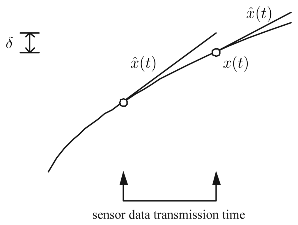
Figure 2.
Send-on-delta transmission with a linear predictor
2.1. New send-on-delta algorithm with a linear predictor
The proposed algorithm is given in Fig. 3 and Fig. 4. In the sensor node, it is assumed that the sensor node is sampled with the period T. A discrete-time signal xk is defined by xk = x(kT). Even if the sensor value is sampled with the period T, the actual transmission rate is not T since not all sampled sensor data are transmitted.
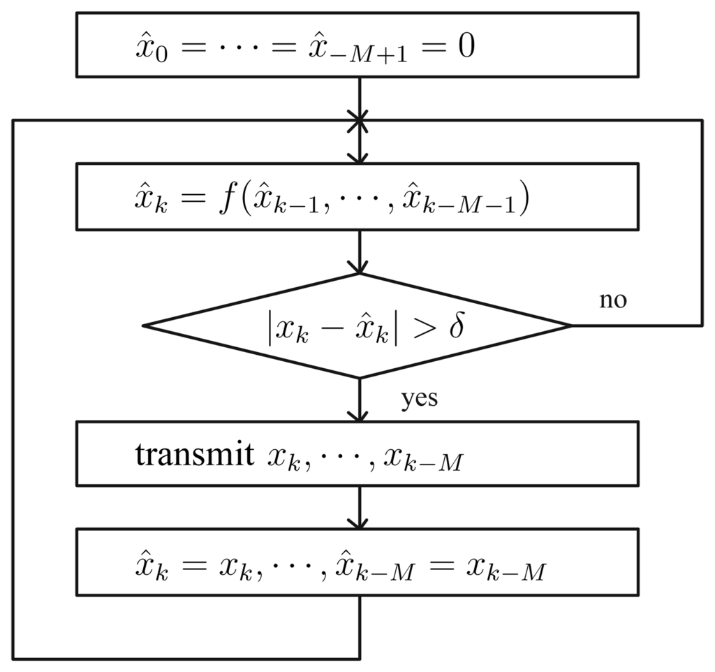
Figure 3.
Transmitter Algorithm in Sensor Nodes
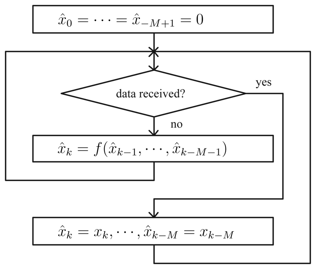
Figure 4.
Receiver Algorithm in the Monitoring Station
In the sensor node, x̂k = f(x̂k−1, ⋯, x̂k−M−1) indicates a linear predictor, where M denotes the memory length. If M = 1, x̂k is computed based on x̂k−1 and x̂k−2. How to choose a linear predictor f (·) is discussed later. Note that we use f (x̂k−1, ⋯, x̂k−M−1) instead of f (xk−1, ⋯, xk−M−1). If we used f (xk−1, ⋯, xk−M−1), we would have obtained more accurate x̂k; however in that case we have to transmit xk to the monitoring station at every T seconds. Thus we cannot reduce the number of transmission.
If the difference between the current value xk and the predicted value x̂k is larger than δ, we transmit xk, ⋯, xk−M instead of just transmitting xk. Why we have to transmit xk, ⋯, xk−M is discussed in Section 4. In the conventional send-on-delta method, we only need to transmit xk. In this sense, the transmission data size is larger than that of the conventional send-on-delta method. Despite this, we will see later in Section 4 that the overall network overhead of the proposed method is significantly smaller than the conventional send-on-delta method.
In the monitoring station, when sensor values are not received, we predict the current sensor value using a linear predictor x̂k = f(·). From the transmitter algorithm, it is guaranteed that the error between xk and x̂k is smaller than δ.
2.2. Linear predictor
If a signal is a random process with a known distribution, we can obtain an optimal predictor [12]. In this paper, we assume that we have no information about the signal which we measure.
To derive a predictor equation, consider the Taylor expansion of a signal:
If we take two terms from the right hand sides of (1) and apply Euler approximation (ẋ(kT) ≈ (x(kT) − x((k − 1)T))/T), we obtain the following:
This is a first order predictor for xk = x(kT); this corresponds to M = 1 in the algorithm of Fig. 3 and Fig. 4. Similarly, we can obtain a second order predictor for xk = x(kT).
We could go further to obtain higher order predictors. However, as we will see in Section 4, the use of higher of predictors does not reduce the number of transmission rate. Thus in this paper, we will mainly use the first order predictor (2) as a linear predictor f(·).
3. Mean rate of messages analysis
In this paper, we compute the mean rate of messages (λ). The mean rate of messages is defined as the mean number of transmission per a unit of time. We will show that the mean rate of messages (λ) is dependent on δ and
, which is the time average of ẍ(t).
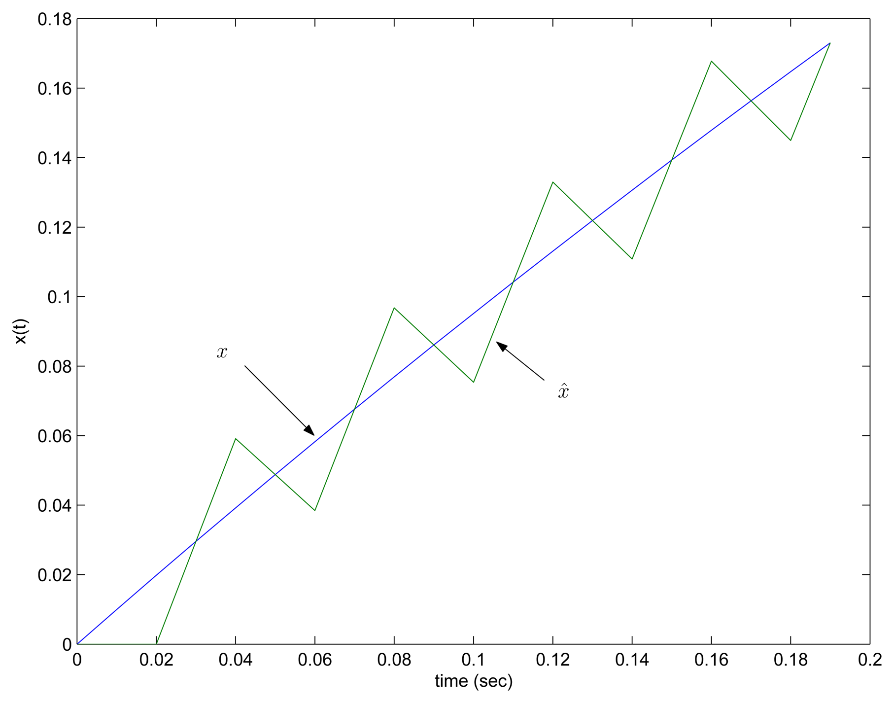
To derive the mean rate of messages, we use the famous mean-value-theorem [13].
Theorem 1 (Mean-Value Theorem) Assume that x has a derivative at each point of an open interval (a, b), and assume also that x is a continuous function at both endpoints a and b. Then there is a point c in (a, b) such that
From Theorem 1, there exists αk (kT < αk < (k + 1)T) satisfying
An example is given in Fig. 5. It is possible that αk is not unique; in that case, we can choose any αk.
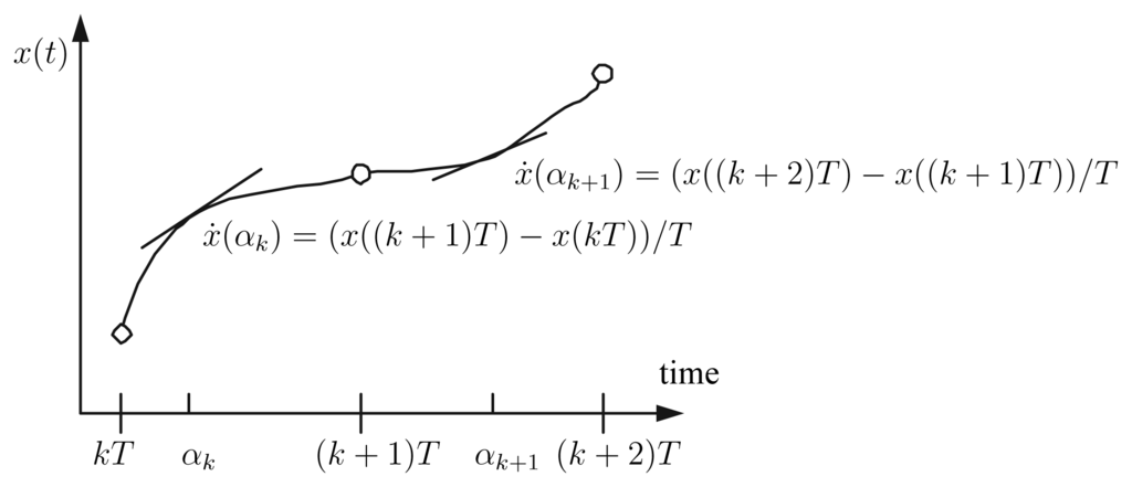
Figure 5.
Mean-value-theorem and αk definition
Assume that the sensor data is transmitted at kT; recall that xk and xk−1 are transmitted for the first order predictor. Thus it is satisfied that x̂k = xk and x̂k−1 = xk−1.
First we investigate E{|xk+N − x̂k+N|} so that we can see how often |xk+N − x̂k+N| exceeds δ. From the definition of αk in (4), we have
In the above equation, we have used the fact that x̂k = xk and x̂k−1 = xk−1. If we proceed to the next time step, we obtain
We used (7) in the fourth row derivation.
Continuing the process, we can obtain a general form as follows:
Note that the time average of αk − αk−1 is T, which can be verified from the following relationship:
Noting that
we have the average value of |x((k + N)T) − x̂((k + N)T)| as follows
where
is the time average of |ẍ(t)|.
Let Nmax be the maximum value satisfying (T is given)
Then λ, the mean rate of messages, satisfies the following:
For three different algorithms (the periodic sampling, the conventional send-on-delta method, the proposed method), mean rates of messages are compared in Table 1. For all three algorithms, the error in the remote station is less than δ; that is, the estimation performance is the same. Thus smaller λ implies that the estimation performance can be achieved with less frequent transmission of sensor data.

Table 1.
Mean rate of messages comparison for 3 different algorithms
We can see that in Table 1 that λ of the proposed method depends on
while λ is dependent max ẋ (periodic sampling) and
(send-on-delta method). For slowly varying signals, we have the following relationships in general:
Thus we can expect that the proposed method has the smallest number of transmission. This expectation is verified in the next section.
4. Simulation
To verify the proposed algorithm, we applied the proposed algorithm to four control signals, which are typical control system responses. The signals are given in Table 2, where one is a step response of a first-order system and the others are step responses of second-order systems. These signals are used in [8] and we used the same signals to compare effectiveness of three algorithms.
Table 2.
Four signals for the number of transmission test
Mean rates of messages (λ) in the case of δ = 0.02 are given in Table 3, where λ is computed using equations in Table 1. For the send-on-delta method and the proposed method, upper bounds of λ are used. Note that the estimation performance for three algorithms are the same in the sense that the worst case error is δ. Thus small λ means that we can achieve the same estimation performance with small number of sensor data transmission.
Table 3.
mean rate of messages (λ) comparison with δ = 0.02
As can be seen in Table 3, λ of the send-on-delta method is significantly smaller than that of the periodic sampling. And λ of the proposed method is significantly smaller than that of the send-on-delta method. Thus we could expect that the number of sensor data transmission is the smallest if we use the proposed method.
Actual number of sensor transmission is given in Table 4 for the time interval [0, 5] seconds. We chose the final time 5 seconds since the settling times of x1, x2, and x3 are all 5 second. For the oscillating signal x4, 5 second corresponds to a quarter cycle.
Table 4.
Number of sensor data transmission (0 ≤ t ≤ 5, δ = 0.02)
As expected from Table 3, the proposed method has the smallest number of transmission. We used both the first-order predictor and the second-order predictor. Interestingly, there is almost no reduction of transmission number when we use the second-order predictor. For x1, x2, and x4, the numbers of transmission are the same. There is just one transmission reduction for x3. Thus we believe that the first-order predictor is good enough for most signals.
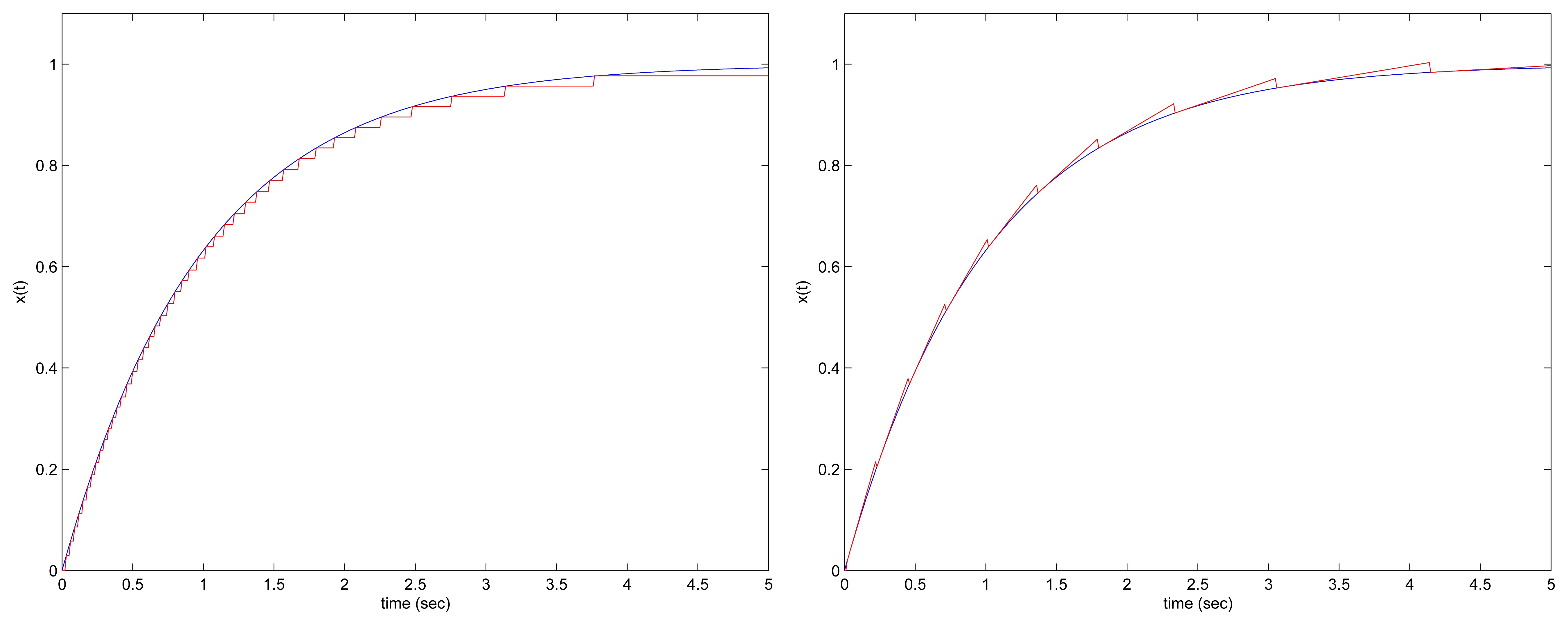
To see how the send-on-delta method and the proposed method work, x1 plots are given in Fig. 6. The left plot is the result of the send-on-delta method and the right plot is the result of the proposed method.
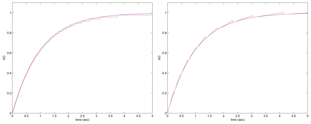
Figure 6.
x1(t) plot with the send-on-delta method (left) and the proposed method (right)
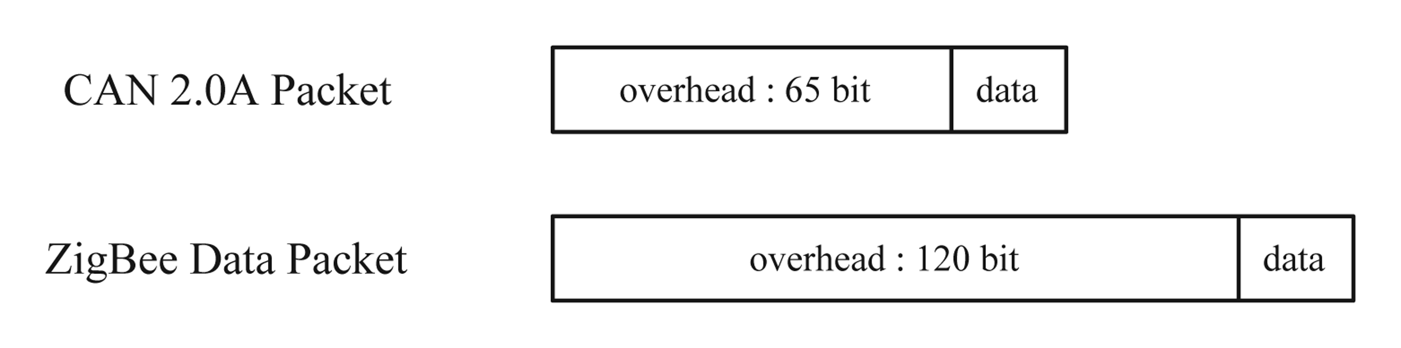
Note that in the proposed method, we have to transmit xk and xk−1, while only xk is transmitted in the periodic sampling and the send-on-delta method. The impact of this increase on the overall network transmission is small since a packet-based transmission is used in most networks. For example, in CAN 2.0A network [14], the packet overhead is at least 65 bits and in ZigBee [15], it is at least 120 bits.
Assuming xk is encoded in 8 bits, total numbers of transmitted bits can be computed as in Table 5.
Table 5.
Total number of transmitted bits computation formula
Using the formulas in Table 5, we can compute the total number of transmitted bits, which is given in Table 6. We can verify that the proposed method transmits much smaller number of bits despite the fact that both xk and xk−1 should be transmitted.
Table 6.
Total number of transmitted bits
Finally we note that it is a bad idea transmitting only xk instead of transmitting xk and xk−1 in the proposed algorithm. In most cases, a predictor output would be oscillating and thus the number of transmission becomes very large. An example is given in Fig. 8. We can see the oscillation phenomenon and the number of transmission is 250 while only 11 for the proposed method.
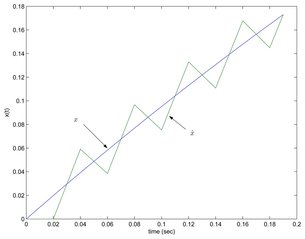
Figure 8.
Oscillation problem when only xk is transmitted (x1(t) with δ = 0.02)
5. Conclusion
In this paper, we have proposed a new sensor data transmission algorithm, which reduces the number of transmission. A linear predictor is used to predict the sensor value and the sensor data are transmitted if the difference between the predicted sensor data value and the current sensor value exceeds specified δ. With little increase in the computational burden in the sensor nodes, we can significantly reduce the number of transmission. We believe the proposed algorithm is useful for sensor networks (for battery power saving) and networked control systems (when a bandwidth for sensor data is limited).
Acknowledgments
This work was supported by grant No. R01-2006-000-11334-0 from the Basic Research Program of the Korea Science & Engineering Foundation.
References
- Oppenheim, A. V.; Schafer, R. W.; Buck, J. R. Discrete-Time Signal Processing.Prentice Hall, 2nd edition; 1999. [Google Scholar]
- Walsh, G. C.; Ye, H. Scheduling of networked control systems. IEEE Control Systems Magazine 2001, 21(1), 57–65. [Google Scholar]
- Yang, T. C. Networked control system: a brief survey. IEE Proc.-Control Theory Appl. 2006, 153(4), 403–412. [Google Scholar]
- Zhao, F.; Guibas, L. Wireless Sensor Networks; Elsevier, 2004. [Google Scholar]
- Feeney, L. M.; Nilsson, M. Investigating the energy consumption of a wireless network interface in ad ad hoc networking environment. Proceedings of IEEE Infocom 2001, Anchorage, U.S.A. 2001; pp. 1548–1557. [Google Scholar]
- Miskowicz, M. Analytical approximation of the uniform magnitude-driven sampling effectiveness. Proc. of IEEE International Symposium on Industrial Electronics, Ajaccio, France; 2004; pp. 407–410. [Google Scholar]
- Otanez, P. G.; Moyne, J. R.; Tilbury, D. M. Using deadbands to reduce communications in networked control systems. Proceedings of the American Control Conference, Anchorage, U.S.A. 2002; pp. 3015–3020. [Google Scholar]
- Miskowicz, M. Send-on-delta concept: An event-based data reporting strategy. Sensors 2006, 65, 49–63. [Google Scholar]
- Suh, Y. S.; Nguyen, V. H.; Ro, Y. S. Modified Kalman filter for networked monitoring systems employing a send-on-delta method. Automatica 2007, 43(2), 332–338. [Google Scholar]
- Astrom, K. J.; Bernhardsson, B. M. Comparison of Riemann and Lebesgue sampling for first order stochastic systems. Proc. of the 41st IEEE Conference on Decision and Control, Las Vegas, U.S.A. 2002; pp. 2011–2016. [Google Scholar]
- Plonnigs, J.; Neugebauer, M.; Kabitzsch, K. A traffic model for networked devices in the building automation. 2004 IEEE Internatinoal Workshop on Factory Communication Systems; 2004; pp. 137–145. [Google Scholar]
- Gersho, A.; Gray, R. M. Vector Quantization and Signal Compression.; Kluwer Academic Publishers, 1992. [Google Scholar]
- Apostol, T. M. Mathematical Analysis.; Addision-Wesley Publishing Company, 1974. [Google Scholar]
- Lawrenz, W. CAN System Engineering : From Theory to Pratical Applications.; Springer Verlag: New York, 1997. [Google Scholar]
- Zigbee-Alliance. Network Specification, Version 1.; 2004. [Google Scholar]


© 2007 by MDPI ( http://www.mdpi.org). Reproduction is permitted for noncommercial purposes.