Abstract
The aim of the present study was to develop an electronic nose for the quality control of red meat. Electronic nose and bacteriological measurements are performed to analyse samples of beef and sheep meat stored at 4°C for up to 15 days. Principal component analysis (PCA) and support vector machine (SVM) based classification techniques are used to investigate the performance of the electronic nose system in the spoilage classification of red meats. The bacteriological method was selected as the reference method to consistently train the electronic nose system. The SVM models built classified meat samples based on the total microbial population into “unspoiled” (microbial counts < 6 log10 cfu/g) and “spoiled” (microbial counts ≥ 6 log10 cfu/g). The preliminary results obtained by the bacteria total viable counts (TVC) show that the shelf-life of beef and sheep meats stored at 4 °C are 7 and 5 days, respectively. The electronic nose system coupled to SVM could discriminate between unspoiled/ spoiled beef or sheep meats with a success rate of 98.81 or 96.43 %, respectively. To investigate whether the results of the electronic nose correlated well with the results of the bacteriological analysis, partial least squares (PLS) calibration models were built and validated. Good correlation coefficients between the electronic nose signals and bacteriological data were obtained, a clear indication that the electronic nose system can become a simple and rapid technique for the quality control of red meats.
1. Introduction
The evaluation of quality in red meat products is needed because producers, agents of the logistic chain and vendors need to ensure that they offer products that meet the quality expectations of customers. Additionally safety evaluations of such products are needed because the industry and also regulatory bodies need to ensure that red meat that reaches the market is safe. The shelf-life of meat may be defined as the time elapsing between production and spoilage. The spoilage of meat is a sensorial quality and may consist in the occurrence of off-odours and off-flavours or discoloration [1-3]. In red meats, the off-odours resulting from bacterial activity determine their shelf-life. It is generally accepted that detectable organoleptic spoilage is a result of decomposition and the formation of metabolites caused by the growth of microorganisms [4]. It is known that a post-mortem endogenous enzymatic activity within muscle tissue can contribute to significant changes during meat storage [5]. Consumption of spoiled meat products could cause serious health hazards. Since sensory analysis is very expensive and not always possible, developing automated sensing techniques able to ensure the safety and quality of meat products is a priority task and would benefit both producers and consumers. This is why many efforts are underway or have been conducted to develop different types of sensors for meat quality or safety applications [6].
The reference method currently used for determining the spoilage status of meat is analysing the total count of bacteria and/ or specific spoilage bacteria. An obvious drawback with such a bacteriological method is the incubation period of 1–2 days that is required for colony formation and, additionally, the lack of correlation between the degree of spoilage (from the sensorial point of view) and the total count of bacteria that is often observed [3]. Although, bacterial growth on meat samples has been extensively studied, methods based on the total count of bacteria that correlate well with shelf-life determination are still under investigation [7]. In spite of its drawbacks, bacteriological methods can be employed in many cases to define the desired product quality and are a good indicator of product safety. Furthermore, the results obtained from a bacteriological analysis can then be used to train alternative methods such as an electronic nose system [7].
Some chemical compounds may be used as spoilage indicators. In previous studies, acetate, alcohols, H2S have been put forward as possible spoilage indicators in vacuum-packaged meat and meat products [7, 8] while acetone, methyl ethyl ketone, dimethyl sulphide or dimethyl disulphide appear in meats kept under cold storage in the presence of oxygen [4]. However, the use of a few chemical compounds as spoilage indicators in meat (i.e., their quantitative analysis) involves laborious sampling, extraction and analysis procedures.
Quality and safety control of red meats may also be performed using an electronic nose system. According to Gardner and Bartlett [9], the electronic nose is an instrument which comprises an array of electronic chemical sensors with partial specificity and an appropriate pattern recognition system, capable of recognising simple or complex odours. In order to classify samples, an electronic nose combines the response profiles of various sensors, which react to different types of volatile compounds in the odour. Many groups are attempting to develop an electronic nose for the quality control of red meat [10-13].
In this paper, an electronic nose is used to assess the quality of beef and sheep meats stored at 4 °C. The purpose of this study is to evaluate the electronic nose performance as an additional instrument for the quality/ safety control of beef and sheep meats. To perform an objective evaluation of the artificial olfactory system, it is absolutely necessary to compare its predictions against bacteriological results since, nowadays, although far from perfect, bacteriological tests are the only generally accepted way to estimate the shelf life of meat in an objective manner.
2. Experimental
2.1. Sample preparation and sampling
Two different types of meat species representative of Moroccan production and purchased from a local market were analysed. The samples from different animal species (beef and sheep) were cut into pieces of the same weight (10 g ± 1 g) immediately after receiving, placed in plastic bags (bags for freezing food) and introduced in a refrigerator kept at a constant temperature of 4°C ± 1°C. For each measurement, a meat sample was taken from the refrigerator and put inside a 500 ml glass bottle. The sampling bottles were sealed with septum and held at room temperature (22°C ± 2°C) for 50 min in order to reach a stable composition of the headspace. Measurements were performed each day for up to 2 weeks. Every day two replicate samples were withdrawn from the refrigerator to undergo microbiological analysis and six replicate samples were employed for electronic nose analysis. This procedure was repeated with the two types of red meats under investigation.
2.2. Microbiological population enumeration
A 25 g sample of each product was taken aseptically and placed in a sterile stomacher bag containing 225 ml of 0.1 % (wt/vol) peptone water (PW, Oxoid Ltd., Hampshire. England). The sample and the PW were stomached for 2 min. Decimal dilutions were prepared using the same diluent. These dilutions were subsequently plated on the surface of a Plate Count Agar (PCA, Oxoid Ltd.). The plates were incubated at 30 °C for 2 days. The total viable counts (TVC) were obtained by enumerating the colonies present, and calculated as log10 colony forming units (cfu)/g of the sample.
2.3. Electronic nose system
An electronic nose system was employed to obtain the smell patterns from the headspace of meat samples (Fig. 1). This electronic nose system contains an array of six tin oxide based Taguchi gas sensors obtained from Figaro Engineering, a temperature sensor (National Semiconductors LM35DZ), and humidity sensor (PHILIPS H1). The identification codes of the Figaro sensors that were used are as follows (their target gases, as suggested by the manufacturer, are also indicated): TGS 823 (Alcohols, Xylene and Toluene), TGS 825 (H2S), TGS 826 (NH3), TGS 831 (Chlorofluorocarbons), TGS 832 (Halocarbons) and TGS 882 (Alcohols) [14]. The TGS sensors from the 8 series have been used by other authors in the quality control of red meats [13]. These sensors, which are based on tin oxide doped with noble metal catalysts show good responsiveness to acetone, and nitrogen and sulphur compounds, which have been suggested as spoilage indicators for read meat [4, 7, 8]. Full details on the electronic nose system implemented here can be found elsewhere [15].
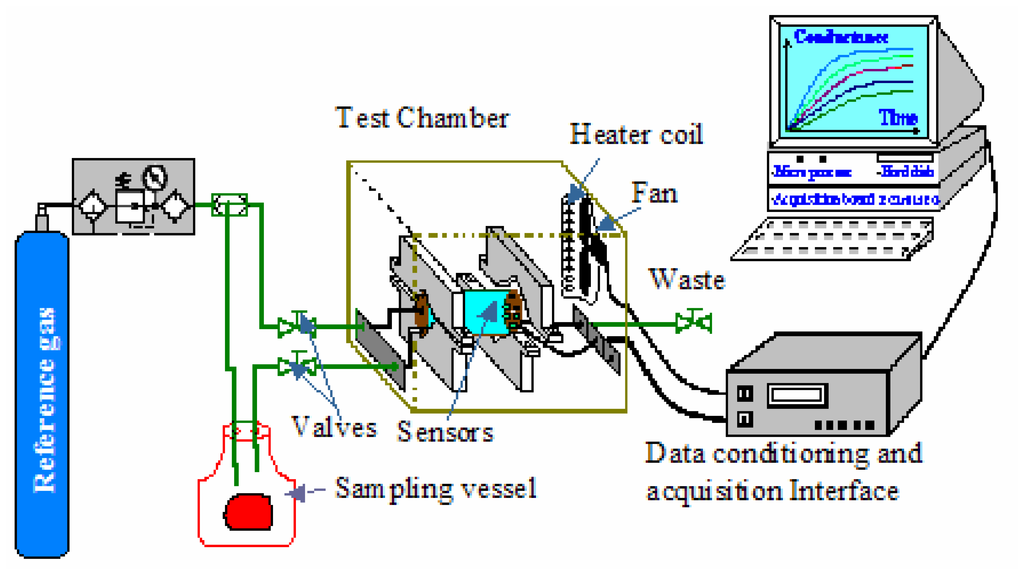
Figure 1.
Schematic of the experimental set-up.
In a typical measurement, the headspace from a meat sample is fluxed into the electronic nose sensor chamber. Pure nitrogen is used at a constant flow of 500 sccm to allow the volatile species from the headspace to reach the sensor chamber. The electronic nose response is sampled (1 sample/s) for a time interval of 50 min. After the 50 min measurement, nitrogen is flushed again to clean the system until the steady state baseline resistance of the sensors is reached.
The variation of the sensors' conductivity is acquired and then digitised using a data acquisition board (PCL 812PG, Advantech). A program in LabVIEW was developed to control the data acquisition process.
Data processing and pattern recognition are decisive factors in order to obtain a versatile instrument able to reliably recognize a wide variety of odours. MATLAB 6.5 software is used for pre-processing and data analysis.
2.3.1. Feature extraction and pre-processing
To calculate the sensor response to the headspace of a meat sample, the following expression was used:
where G is the response, GN the value of the conductance in nitrogen, GM is the value of the sensor conductance in the presence of the meat sample and M is the weight of the meat samples being measured.
The features used for data analysis are extracted from the temporal responses of the sensor array (i.e. from the temporal evolution of G). Fig. 2 shows an example of the temporal responses of the sensor array at day 9 for beef and sheep meats. From these sub-plots, which represent the conductance variation of the sensor array (as defined by Eq. 1), a slight variation in conductance is observed during the first 15 minutes of exposure. Then, a sharp increase in conductance occurs in the time interval between 15 and 40 minutes. Finally, the responses show a tendency to stabilise. To better exploit the information obtained from each experiment, a set of additional features that can be extracted from sensor response was employed. Therefore, for every sensor within the array and measurement performed, four representative features from the response signal are extracted. These are:
- G0: the initial conductance of a sensor calculated as the average value of its conductance during the first 15 minutes of a measurement (using the definition in Eq. 1).
- Gs: the steady-state conductance calculated as the average value of its conductance during the last 5 minutes of a measurement.
- dG/dt: the dynamic slope of the conductance calculated between minute 15 and 35 of a measurement. This corresponds to a phase where a fast increase of sensor conductance is observed.
- A: the area below the conductance curve in a time interval defined between 15 and 40 min of a measurement. This area is estimated by the trapeze method.

Figure 2.
Time responses of an array of six gas sensors at day 9 for beef (a) and sheep meats (b).
Extracting the four aforementioned features from each sensor response and pre-processing the resulting data matrix was an automated process via a written-in-house MATLAB 6.5 program. Following the procedures described above, 84 measurements were performed for each meat product, which corresponded to six replicate measurements per storage day during 14 days. Therefore, the original data matrix had 84 rows (i.e., measurements) and 24 columns (i.e., 6 sensors × 4 response features/sensor). The datasets were pre-processed using an auto-scaling procedure when principal component analysis (PCA) was employed. In all data analysis, the datasets were normalised to set their range to (0, 1) when PCA or SVM were used.
The occurrence of drift in the sensor signals was not measured explicitly, since no measurements with a calibrated gas were performed during the 14-day measurement phase. However, no significant response drift was observed during this experimental period for the raw value of the sensors' resistance measured in the presence of the reference gas. Even though some slight upward or downward random variation in the baseline resistance could be detected, a trend could not be identified for these variations and, therefore, it can be considered that drift was negligible during the whole measurement phase.
2.3.2. Data analysis
2.3.2.1. Principal component analysis (PCA)
This method is a powerful linear unsupervised pattern recognition method which is usually successfully used in gas sensor applications [16, 17]. Generally, the PCA method reduces the dimensionality of a multivariate problem. In fact, this method consists in extracting features by projecting the high-dimensional data set in a dimensionally reduced space constituted by the uncorrelated and orthogonal eigenvectors of the covariance matrix computed from the sensor responses, called principal components. The magnitude of the single eigenvector or percentage of ‘’information” is expressed by the own eigenvalue, which gives a measure of the variance related to that principal component.
2.3.2.2 Partial least squares regression (PLS)
In order to compare the electronic nose performance with a bacteriological technique, measurements were performed concurrently with both techniques. PLS models were used to describe the relationships between the results of the two techniques and to make predictions on the quality of samples. Unlike PCA, PLS is a supervised method: it includes information that helps to obtain a score plot best describing the known differences between the samples [18]. It is a prediction method that consists of three steps: model building, model validation with known samples, and prediction of unknown samples. In the strategy that was employed here, during the training phase, the PLS algorithm built a model that described the relationship between sensor signals and microbial counts. In the evaluation phase, the model predicted microbial counts using new electronic nose measurements that had not been used for training.
In other words, PLS regression models were built for the TVC in beef and sheep using the electronic nose responses s as input data and the microbiological counts as output data.
2.3.2.3. Support vector machines (SVM)
Support vector machines [19] are a core machine learning technology. SVM were originally designed for binary classification. How to effectively extend it for multi-class classification is still an on-going research issue. Several methods have been proposed where typically a multi-class classifier is constructed by combining several binary classifiers.
In this section we discuss briefly the one versus one approach. It was first introduced in [20] for training neural network based classifiers, and the first use of this strategy on SVM was reported in [21], [22]. This method trains ½M×(M - 1) binary SVM models, where each one is trained on data from two classes and M is the number of classes. To classify a data object, the one vs. one approach combines the scores of these ½M×(M - 1) classifiers. Each of the ½M×(M - 1) binary SVM classifiers provides a partial decision for classifying a measurement. There are different methods of combining the results obtained from the classifiers, among which, the most common is a simple voting scheme [21]. When classifying a new instance, each one of the base classifiers casts a vote for one of the two classes used in its training.
3. Results and Discussion
3.1. Bacterial analysis
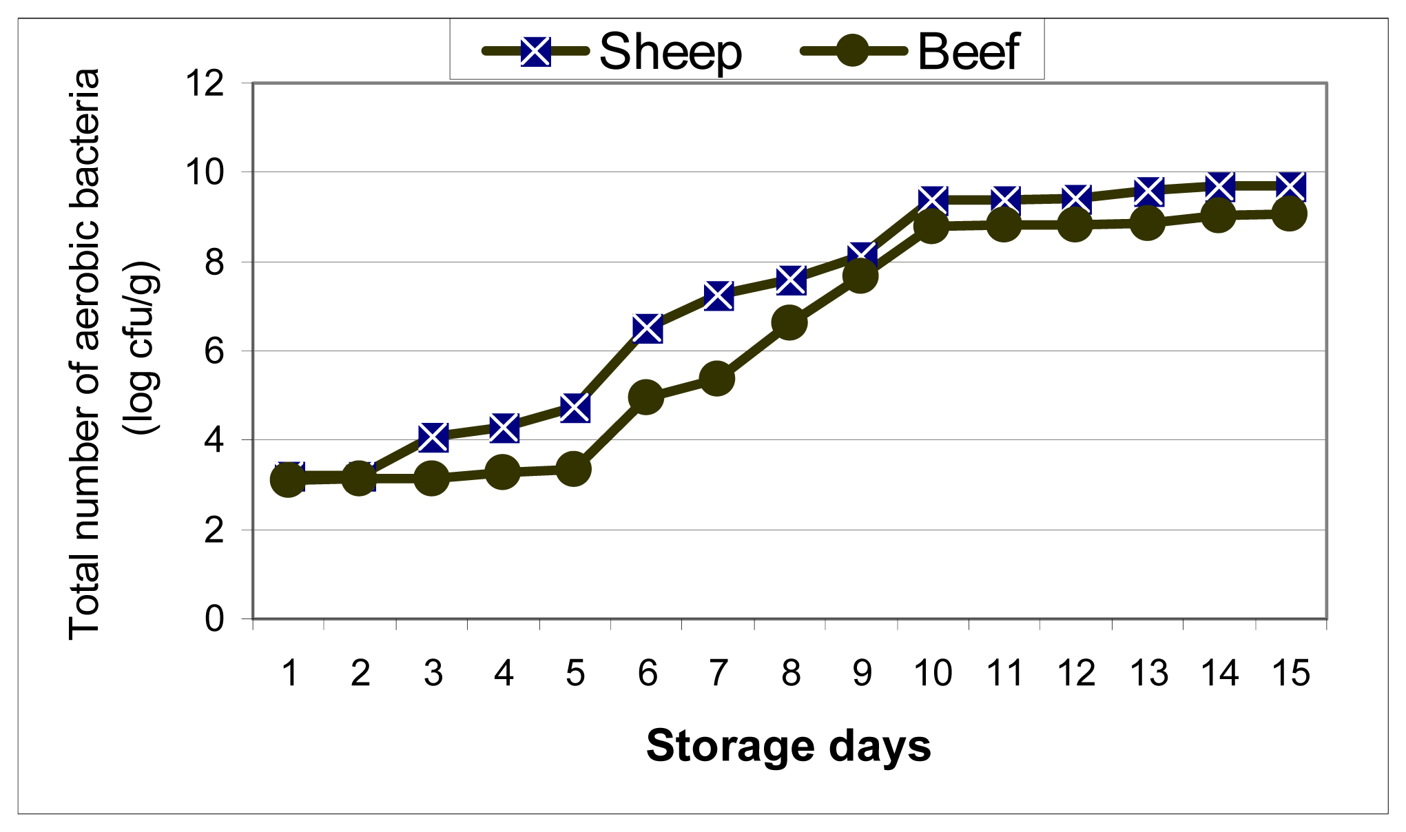
The results of the bacterial analysis performed on the red meats, which were used in the development of the classification models with the electronic nose, are presented in Fig. 3. This figure shows the evolution of log10 cfu/g developed in the two types of meat as a function of the days of cold storage. It was decided that a quality criterion corresponding to a 106 cfu/g for TVC should be applied to discriminate between unspoiled and spoiled samples in this study, because this is the general microbiological safety guideline applied for food quality [13, 23, 24]. A similar behaviour was observed for the two types of meat analysed. The TVC shows a slight variation in the first five days followed by a very fast increase between days five and ten, and finally in the last days of conservation the curves show a tendency to stabilize. For the first five storage days, the two TVC for beef and sheep meats are near 3 log10 cfu/g and 4 log10 cfu/g, respectively. That is, just after slaughter beef or sheep meat samples were already contaminated by bacteria at a level lower than 3.5 log10 cfu/g. During this initial storage period, bacteria did not proliferate rapidly. However, when storage time further increased, bacteria increased rapidly and reached 8.8 log10 cfu/g in beef and 9.37 log10 cfu/g in sheep samples after ten days. When storage time increases, the level of nourishing elements increases in meat and this could explain the growth of bacteria. Fig. 3 indicates that the deterioration of meat quality starts from days four or five, when meat is stored at 4 °C. The meat, which contains bacteria at a level of less than 5 log10 cfu/g, is said to be acceptable for consumption. However, the meat is spoiled and not suitable for consumption when viable counts exceed 6 log10 cfu/g. At this stage, a putrid smell was released from the meat. In addition, it can be noticed from Fig. 4 that the TVC increases at a slightly faster pace in sheep than in beef meat. This can be explained by the fact that sheep meat contains more proteins and lipids than beef meat [25]. It can be noticed also that the threshold of consumption acceptability (i.e., microbial counts < 6 log10 cfu/g) [13] is reached at day seven for beef meat and at day five for sheep meat.
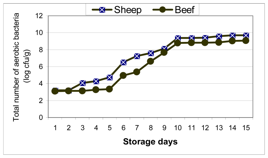
Figure 3.
Changes in the count of aerobic bacteria.

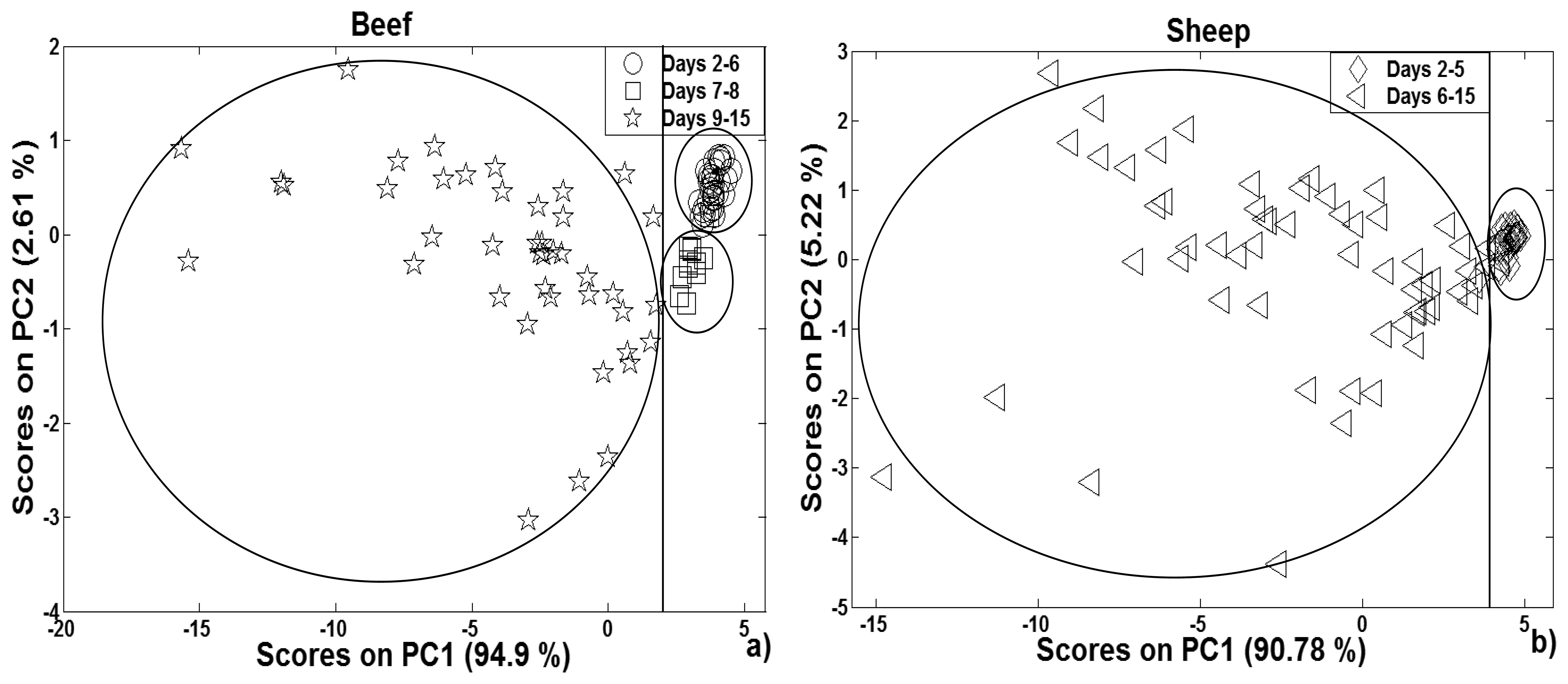
Figure 4.
Scores plot of a PCA on beef meat (a) and sheep meat (b).
3.2. Electronic nose analysis
3.2.1. PCA analysis
In parallel to the bacteriological analysis, an analysis employing the electronic nose system was made. In the first step a PCA was used as an unsupervised classification method to visualize the resemblance and the difference among the different measurements in the datasets. In the second step, the method was employed to compare the deterioration speed between beef and sheep meats.
Fig. 4 shows the score plot of the data in the PC1-PC2 plane for beef and sheep meats. For beef meat (Fig. 4-a) it can be noticed that the measurements cluster together in three different groups. The first group corresponds to samples having undergone up to 6 days of storage. The second group corresponds to the samples having undergone from 7 up to 8 days of storage. Finally, the third group corresponds to samples that underwent from 9, up to 15 days of storage. However, the bacteriological analysis shows that beef meat stored 7 and 8 days should be considered as unspoiled and spoiled, respectively. So, it is difficult to reach a correct determination of shelf-life for beef meat by using a PCA method. For sheep meat (Fig. 4-b) it can be noticed that the dataset measurements are grouped in two groups. The measurements corresponding to the first five storage days formed the first group and the measurements corresponding to 6-15 storage days formed the second one. In this case the PCA method shows a good separation between unspoiled and spoiled sheep meats. So, the method could be used for the rapid shelf-life determination of sheep meat.
In order to compare the speed of deterioration between beef and sheep meats, the scores on PC1 were employed. Fig. 5 shows the evolution of the scores on the first principal component PC1 as a function of storage time and its polynomial fitting for the case of beef and sheep meats. These scores show a monotonic decrease during the period of storage. A slight variation in the first five storage days followed by a very fast decrease of the scores on PC1 in the last storage days can be seen. It is observed that PC1 mainly describes the change in the degree of meat spoilage [12]. It can be noticed that the spoilage of sheep meat is faster than that of beef meat, which is in good agreement with the bacteriological analysis results.
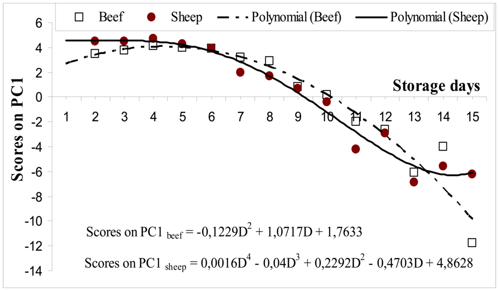
Figure 5.
Evolution of the scores on the first principal component with the period of storage and polynomial fitting for beef and sheep meats.
3.2.2. SVM analysis
A supervised pattern recognition method such as SVM was employed for classification tasks. SVM was applied to test he ability of the electronic nose set-up for separating between unspoiled and spoiled beef or sheep meat. SVM with the multi class approach one vs. one was used to develop a rule of decision to classify the observations of the dataset into spoiled or unspoiled samples. Taking into consideration the bacteriological analysis results, we divided the dataset in two categories defined as unspoiled and spoiled. As in the PCA, 24 response features from the sensor array were used as inputs to the SVMs. Different kernel function were tested in order to check the robustness of the classifier model. Finally, second- order polynomial kernel function were used to project the training data to a space that maximized the margin hyperplane (i.e., the separation between spoiled and un-spoiled samples). The optimal regularization parameter of the SVM was set to C = 50. This value was found experimentally by minimizing the leave-one-out error over the training set, which provides an estimate of the generalization performances of the final classifier. The kernel parameters and the value of the constant C determine the complexity of the SVM solution and hence, its generalization ability.
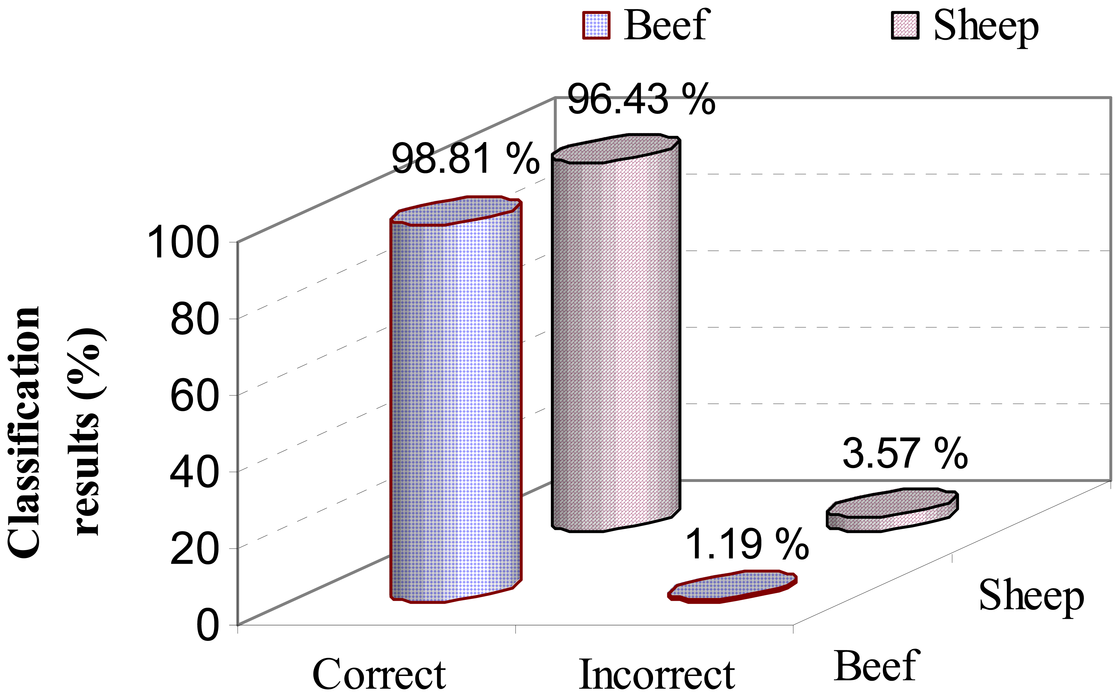
The performance of the final SVM model was evaluated using a leave-one-out cross-validation method. The process was as follows: given n measurements (n = 84 measurements within each training matrix), the model was trained 84 times using 83 vectors. The vector left out was then used for testing the model. Performance in training was estimated as the averaged performance over the 84 tests. A very good success rate in classification was obtained in the spoilage classification of beef and sheep meats, (98.81 % and 96.43 %) respectively. Figure 6 shows the performance of the SVM model in the classification of beef and sheep spoilage. For beef meat just one mistake occurred: one measurement belonging to a spoiled sample was misclassified as being unspoiled. For sheep meat three mistakes occurred: one measurement belonging to an unspoiled sample (having undergone 5 days of storage) was misclassified as being spoiled (6 days of storage were predicted) and two spoiled measurements (having undergone 6 days of storage) were misclassified as being unspoiled (5 days of storage were predicted). It is important to stress that these misclassified samples are close to the threshold of acceptability.
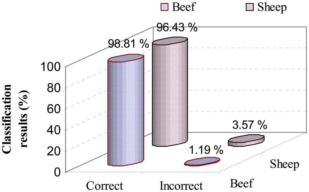
Figure 6.
Performance of the SVM model in the spoilage analysis of beef and sheep samples.
3.3. Correlation between e-nose and bacterial analysis
To investigate whether the results of the electronic nose correlate well with those of bacteriological analysis, different PLS calibration models were built and validated. The underlying objective was to assess if the electronic nose could predict microbial counts (TVC) in beef and sheep meats.
PLS is a linear and supervised multivariate calibration method that attempts to find factors (i.e. latent variables), which capture as much variance as possible in the predictor block X-matrix, under the constraint of being correlated with the predicted block Y-matrix [26].
The X-block consisted in the response matrix acquired with the electronic nose. The Y-block was a column matrix with the results of the bacteriological analysis, i.e. TVC. In this way, the ability of the electronic nose to predict TVC was investigated in beef and sheep meats. The X and Y blocks were mean-centred before the PLS were performed.
The training phase and the prediction ability of the different models built were evaluated. For each meat product, the response matrix, R (84 × 24), was split into different matrices: training matrix and validation matrix.
In fact, three different training and their corresponding validation matrices were used. (i.e. threefold training and validation process). In the first fold, replicate measurements 1 and 2 for each sampling day (i.e. day 2 up to day 15, a total of 14 sampling days) were gathered in the validation matrix V1 (28 × 24) and the remaining measurements were gathered in the training matrix T1 (56 × 24). In the second and third folds the validation matrices used replicate measurements 3 and 4 (V2), and 5 and 6 (V3), respectively. The corresponding training matrices T2 and T3 were formed by the remaining replicate measurements.
The effectiveness of the training process was evaluated calculating the root mean square error of cross-validation (RMSECV) according to the following equation:
where Yi is the actual value of the response and yi the prediction of the PLS-model. Because training is evaluated using a leave-one-out cross-validation, the error is averaged over the N test (N = 56).
The selection of the number of latent variables to build the models was done by representing the evolution of RMSECV versus the number of latent variables. Generally the value of RMSECV decreases when the number of factors is increased and either increases again or stabilises if more factors are added. The number of latent variables selected to build the PLS models the on corresponding to the minimum in the RMSECV.
To better assess the accuracy of the different PLS models, regression between the actual TVC and those predicted by the models was performed. The correlation coefficients were calculated. A perfect prediction would yield 1 as correlation coefficient.
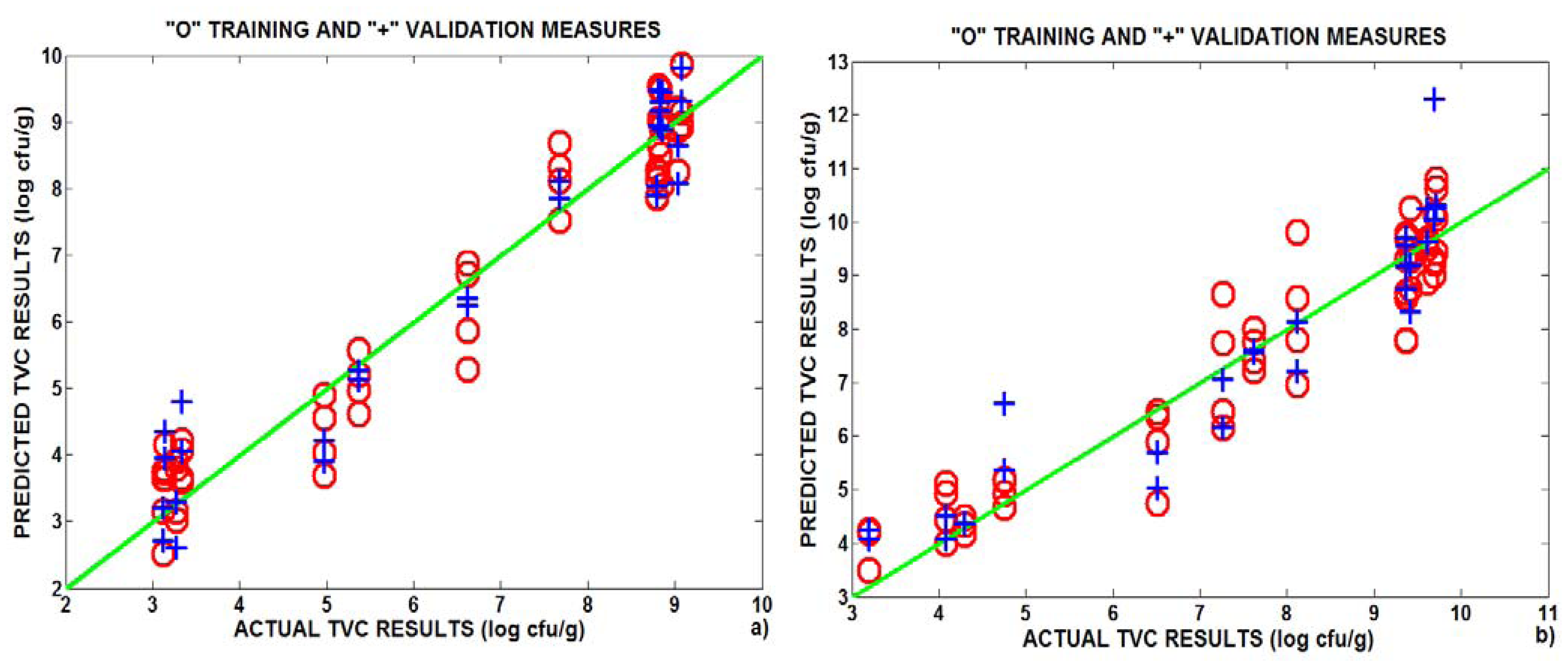
A summary of the average results of this study (for training and validation) for all the PLS models used to predict TVC in beef and sheep meats is shown in Table 1. Fig. 7 shows the predicted TVC with PLS models versus the actual values. The circles are the results of the leave-one-out cross-validation using the training measurements and the crosses correspond to the validation measurements. The predictions for validation measurements (i.e., not used for training) lie in the range of the predictions for training measurements. The numbers of LVs used by the models for beef or sheep meat analysis are 11 and 10, respectively. A very good correlation between the electronic nose results (i.e. sensor response) and bacterial analysis is obtained. In fact, correlation coefficients of 0.89 and 0.84 in training and validation are obtained for beef meat, respectively. Similarly, in the case of sheep meat, correlation coefficients of 0.92 and 0.83 in training and validation were obtained, respectively. This good agreement can be explained because the electronic nose analyses the development of volatile components that result from the bacterial degradation of meat. Since the sensorial spoilage of meat is mostly due to microbial activity, it seems appropriate to use microbial counts as an indicator of meat spoilage [27, 28]. Due to the good correlation existing between the electronic nose response and bacterial counts, the electronic nose could be used as a rapid and alternative way for TVC prediction in red meats.

Table 1.
Training and validation results of the PLS models.
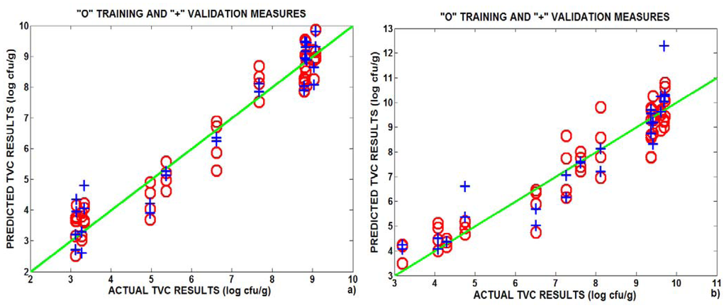
Figure 7.
Results of the PLS models. Actual vs. predicted values of the TVC in beef (a) and sheep meats (b). The circles are the results of a leave-one-out cross-validation performed using training measurements and the crosses correspond to predictions for validation measurements.
4. Conclusion
In the present investigation, a bacterial analysis was used as a complementary method to develop a simple and rapid electronic nose technique for the spoilage classification of red meat. The electronic nose technique, unlike the bacteriological method, has the advantage of being fast and non destructive. The bacterial analysis could be employed to define the self-life of beef or sheep meats, however an obvious drawback with this method is the incubation period of 1–2 days that is required for colony formation.
The effectiveness of the electronic nose in the quality control of red meat was demonstrated in two different applications. First, the electronic nose was used to classify beef and sheep meats according to unspoiled or spoiled. The electronic nose coupled to PCA or SVMs showed very good results for spoilage classification. PCA (a linear technique) could be used to determine the shelf-life of beef meat. However, this was not the case of sheep meat. A very good success rate in the classification of spoiled or unspoiled beef and sheep meats (98.81 and 96.43 %, respectively) was obtained when (non linear) SVM were employed. In the second step, the electronic nose was used to predict the results of the TVC by building quantitative PLS models. The correlation between our electronic nose and the bacteriological analysis was investigated. A good correlation existed between the electronic nose and bacteriological analysis results (the correlation coefficients for beef meat in training and validation were (0.89 and 0.84) and for sheep meat were (0.92 and 0.83). Therefore, the electronic nose could be used as a rapid and reliable method for the quality control of red meat.
According to these results, our electronic nose system can become an alternative tool for shelf-life determination (i.e. quality assessment) and spoilage classification (safety assessment) of red meats.
Acknowledgments
Part of this work has been funded by the AECI under project no. A/5390/06.
References and Notes
- Egan, A.F. Lactic acid bacteria of meat and meat products. Antonie Van Leeuwenhoek 1983, 49, 327–336. [Google Scholar]
- Dainty, R.H.; Mackey, B.M. The relationship between the phenotypic properties of bacteria from chill-stored meat and spoilage processes. J. Appl. Bacteriol. 1992, 73, 103S–114S. [Google Scholar]
- Borch, E.; Kant-Muermans, M.-L.; Blixt, Y. Bacterial spoilage of meat and cured meat products. Int. J. Food of Microbiol. 1996, 33, 103–120. [Google Scholar]
- Stutz, H.K.; Silverman, G. J.; Angelini, P.; Levin, R. E. Bacteria and other volatile compounds associated with ground beef spoilage. Journal of Food Science 1991, 56, 1147–1153. [Google Scholar]
- Schreurs, F.J. G. Post-mortem changes in chicken muscle. Worlds Poultry Science Journal 2000, 56, 319–346. [Google Scholar]
- Yano, Y.; Numata, M.; Hachiya, H.; Ito, S.; Masadome, T.; Ohkubo, S.; Asano, Y.; Imato, T. Application of a microbial sensor to the quality control of meat freshness. Talanta 2001, 54, 255–262. [Google Scholar]
- Panigrahi, S.; Balasubramanian, S.; Gu, H.; Logue, C.; Marchello, M. Neural-network-integrated electronic nose system for identification of spoiled beef. LWT 2006, 39, 135–145. [Google Scholar]
- Borch, E.; Agerhem, H. Chemical, microbial and sensory changes during the anaerobic cold storage of beef inoculated with homofermentative Lactobacillus sp. or a Leuconostoc sp. Int. J. Food Microbiol. 1992, 15, 99–108. [Google Scholar]
- Gardner, J.W.; Bartlett, P. N. A Brief History of Electronic Noses. Sensors Actuators B 1994, 18, 211–220. [Google Scholar]
- El Barbri, N.; Bouchikhi, B.; Llobet, E.; El Bari, N.; Correig, X. Differentiation of red meat using an electronic nose based on metal oxide semiconductor sensors and support vector machines. International Symposium on Olfaction and Electronic Nose ISOEN'07, Saint-Petersburg, Russia, 3- 5 May 2007; pp. 156–157.
- Rossi, V. V.; Garcia, C.; Talon, R.; Denoyer, C.; Berdagué, J.-L. Rapid discrimination of meat products and bacterial strains using semiconductor gas sensors. Sensors Actuators B 1996, 37, 43–48. [Google Scholar]
- Blixt, Y.; Borch, E. Using an electronic nose for determining the spoilage of vacuum packaged beef. International Journal of Food Microbiology 1999, 46, 123–134. [Google Scholar]
- Panigrahi, S.; Balasubramanian, S.; Gu, H.; Logue, C.M.; Marchello, M. Design and development of a metal oxide based electronic nose for spoilage classification of beef. Sensors Actuators B 2006, 119, 2–14. [Google Scholar]
- O'Connell, M.; Valdora, G.; Peltzer, G.; Negri, R.M. A practical approach for fish freshness determinations using a portable electronic nose. Sensors Actuators B 2001, 80, 149–154. [Google Scholar]
- Amari, A.; El Barbri, N.; Llobet, E.; El Bari, N.; Correig, X.; Bouchikhi, B. Monitoring the Freshness of Moroccan Sardines with a Neural-Network Based Electronic Nose. Sensors 2006, 6, 1209–1223. [Google Scholar]
- Sarry, F.; Lumbreras, M. Gas discrimination in an air conditioned system. IEEE Trans. Instrument. Measurement 2000, 49(4), 809–812. [Google Scholar]
- Gardner, J.W. Detection of vapours and odours from a multisensor array using pattern recognition Part 1. Principal component and cluster analysis. Sensors Actuators B 1991, 4, 109–115. [Google Scholar]
- Geladi, P.; Kowalski, B.R. Partial least squares regression: a tutorial. Anal. Chim. Acta 1986, 185, 1–17. [Google Scholar]
- Vapnik, V. Statistical Learning Theory; Wiley, 1998. [Google Scholar]
- Knerr, S.; Personnaz, L.; Dreyfus, G. Single-layer learning revisited: a stepwise procedure for building and training a neural network. Fogelman, J., Ed.; In Neurocomputing: Algorithms, Architectures and Applications; Springer-Verlag, 1990. [Google Scholar]
- Friedman, J. Another approach to polychotomous classification, technical report. Dept. of Statistics, Stanford Univ., 1996. [Google Scholar]
- Krebel, U. Pairwise classification and support vector machines. Schölkopf, B., Burges, C. J. C., Smola, A. J., Eds.; In Advances in Kernel Methods – Support Vector Learning; Cambridge, MA, 1999; pp. 255–268. [Google Scholar]
- Senter, S.D.; Arnold, J. W.; Chew, V. APC values and volatile compounds formed in commercially processed raw chicken parts during storage at 4 and 13 °C and under simulated temperature abuse conditions. Journal of the Science of Food and Agriculture 2000, 80(10), 1559–1564. [Google Scholar]
- Gram, L.; Ravn, L.; Rasch, M.; Bruhn, J.B.; Christensen, A. B.; Givskov, M. Food spoilage-interactions between food spoilage bacteria. International Journal of Food Microbiology 2002, 78(1–2), 79–97. [Google Scholar]
- Moh'd Abdullah, B. Beef and sheep mortadella: formulation, processing and quality aspects. International Journal of Food Science & Technology 2004, 39, 177–182. [Google Scholar]
- Vinaixa, M.; Llobet, E.; Brezmes, J.; Vilanova, X.; Correig, X. A fuzzy ARTMAP- and PLS-based MS e-nose for the qualitative and quantitative assessment of rancidity in crisps. Sensors Actuators B 2004, 106, 677–686. [Google Scholar]
- Dalgaard, P. Qualitative and quantitative characterization of spoilage bacteria from packed fish. Int. J. Food Microbiol. 1995, 26, 319–333. [Google Scholar]
- Gram, L.; Huss, H. H. Microbiological spoilage of fish and fish products. Int. J. Food Microbiol. 1996, 33, 121–137. [Google Scholar]
© 2008 by MDPI Reproduction is permitted for noncommercial purposes.


