1. Introduction
A conventional optical imager is limited in spatial resolution by the diffraction limit of the telescope aperture [
1]. In practice there are many factors to that limit attempts to improve the resolution by increasing the telescope aperture. Synthetic aperture (SA) techniques that are well known in microwave imaging can increase the resolution beyond the diffraction limit of the receiving aperture. And the spatial terminal resolution of synthetic aperture radar in azimuth is limited by the wavelength of the carrier. Consequently research on the application of SA techniques to the optical domain, enabling fine-resolution, two-dimensional, active imaging at a long range with small diameter optics is of great value.
A number of fundamental but innovative synthetic-aperture experiments in the optical domain were performed [
2-
4]. Some prior research relates to SA processing in optical wavelengths for rotating objects like inverse synthetic aperture radar (ISAR) in microwave [
2]. Some experiments in the principle of synthetic aperture radar (SAR) were successfully demonstrated in laboratory [
3]. If we want to bring the experiments to the outside for long-range application, e.g., air-borne or space-borne synthetic aperture imaging lidar (SAIL), many effects should be taken into account [
5].
Fortunately, we can learn experience from SAR, a mature field that was developed to construct microwave images of high resolution by use of antennas of reasonable size. The spotlight model SAR allows the generation of images with a high geometry resolution. If we make SAIL work in spotlight model, amazing resolution can be obtained. Since the SAIL system uses continuous wave (CW) form while pulses are used in the SAR system [
6], we can not directly make use of conventional SAR techniques like the model that Karr has described in his analysis [
7]. And as a result of the continuous wave, we can not provide a high pulse recurrence frequency (PRF), which will lead to azimuth ambiguity [
8] in the spotlight model of the SAIL system.
In this paper, the FM-CW SAIL signal processing will be addressed and the response to a point target will be developed first. Then, a modified Omega-K algorithm will be derived for the CW signal in the spotlight model. Finally, computer simulation will show the validity of the modified algorithm. Considering the effect of the atmosphere that certainly has potential to do harm to SAIL resolution, the wave distortions caused by atmospheric turbulence will be simulated by means of phase screens, and analysis in provided.
2. FMCW SAIL signal and definition of imaging geometry
This section derives an analytical development of the dechirped signal [here by “dechirped” we mean heterodyning the return chirped signal with a similarly chirped local oscillator (LO)], which is the FMCW SAIL signal in the two-dimensional time domain without using the stop-and-go approximation that is assumed in a conventional pulsed SAR system.
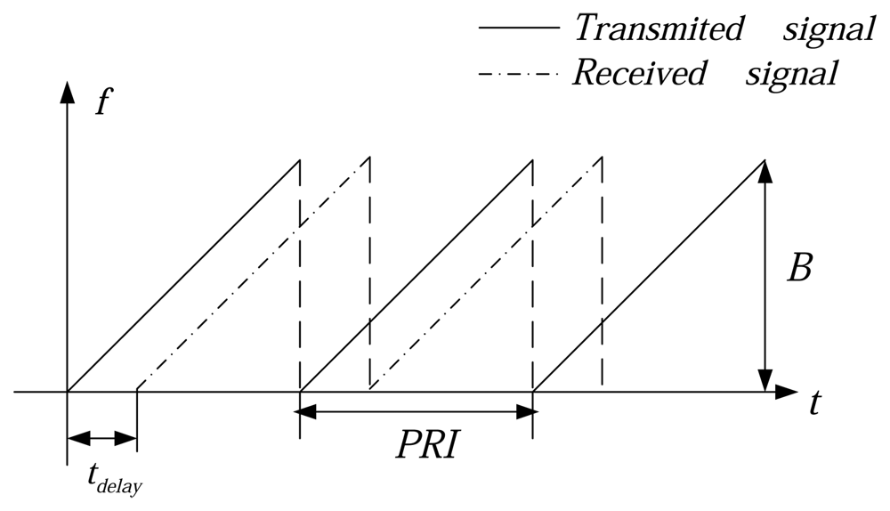
Figure 1 shows the frequency versus time characteristics of the transmitted signal (solid line) and the received signal (dashed line).The received signal is a delayed version of the transmitted one. The lidar continuously transmits linear FM chirps with duration
Tp equal to the pulse repetition interval
PRI and the reciprocal of
PRF. The transmitted signal is expressed as
where −
Tp /2 ≤
t̂ <
Tp /2, the chirp rate
γ=
B/
PRI, where
B is the transmitted bandwidth and
fc is the center frequency. The envelope of the transmitted pulse and the antenna diagram are included in the parameter A with a constant phase but a varying amplitude.
For typical pulsed SAR systems the pulse length Tp is sufficiently short that the radar is assumed stationary during the transmission and the reception of the signal. This is the so-called “stop-and-go” approximation to the case when the platform, such as an aircraft, is flying. It appears as if it stopped, sent a pulse, received it and then moved to the next position. Conventional SAR algorithms make use of this assumption. If the duration of the pulse is increased, the approximation can not be considered valid any more. In the case of FM-CW SAIL, this approximation may no longer be valid because relatively long sweeps are transmitted.
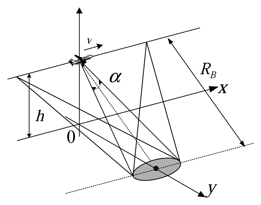
Figure 2 shows the basic geometry of a spotlight mode of a SAIL system. The platform with a transmitter–receiver module moves across the synthetic aperture, namely the azimuth direction, with speed
v perpendicular to the line of sight (LOS), namely the range direction. The beamwidth is
a, the height of the platform is
h, the range from the target center to the sampling aperture pupil antenna phase center (APC) at the closest approach is
RB, and
Rt is the sampling-aperture-pupil-dependent distance to the point target:
where,
vt̂ indicates that the stop-and-go approximation is not valid any more, since
Rt depends only on
tm in a conventional SAR system. Here
tm =
nTp, namely the time of the recording during the synthetic aperture time
Ta, i.e.
. And considering the effect of the atmosphere, we can obtain the value of the phase error through the turbulence in the same way as in [
9,
10].
where,
F is the Fourier transform, Φ(
fx,
fy) is the power spectral density of the refractive index fluctuations of the atmosphere (using the von Karman model) and
r̃0 is the similar coherence length of atmosphere defined by Karr [
4]. The variables
fx and
fy are the spatial frequencies.
f0 = 2
π /
L0, and
L0 is called the outer scale. Due to the fact that the phase error is a nonparametric error, it is hard for us to give the exact expression. In the simulation, we transform the phase error
φ(
x,
y) to the variable Δ
r by
. Therefore
, and
is the real distance form the pupil to the point, which is like the way of dealing with the motion of the platform [
6]. Here, we ignore the phase error (if we choose a right synthetic aperture length) in order to simplify the derivation. Then we replace
by
Rt in the subsequent section, which dose not affect the analysis.
So the received signal can be written as
which is a replica of the transmitted signal delayed by
τ, where
,
c is the speed of light, and 2 stands for the round-trip. In the same way, the reference signal can be written as:
where
, and
Rref could be zero or an arbitrary but fixed value. In this paper, we choose
Rs as the slant range distance of the scene center at boresight position as
Rref. In this heterodyne detection system, the received and the referenced signal (which can be the transmitted signal or its delayed one) are mixed. In the receiver, the received signal is demodulated with the reference signal. The demodulation results in the beat signal
In the equation, the first exponential term is the Doppler modulation in azimuth and the second term represents the range signal, which is a sinusoidal signal with a constant frequency corresponding to the azimuth dependent distance to the point target Rt, and the last exponential term represents the residual video phase (RVP) term, and can be ignored for its long sweeps, i.e., a small chirp rate.
Starting from the square root expression for range
Equation (2), it is useful to make the approximation:
where
. This approximation is valid for a CW model, since the terms higher than the second order in the series expansion
(7) are very small. Then the Doppler shift effect, induced by the continuous motion within the sweep, can be expressed as:
where
λ is the carrier wavelength,
θ is the Doppler cone angle between the antenna velocity vector and the radar line of sight to the target center, and
fa is the Doppler frequency in azimuth right equal to the Doppler shift
fd which must be compensated, otherwise it will affect image location and geometric fidelity, and result in distortion.
In a SAIL system, the effects induced by the continuous motion are very small in
, so they can be replaced by
in
Equation (6). So ignoring RVP through range deskew, the signal becomes:
The term
of the envelope is small compared to the delay of the signal and can be ignored.
The fist exponential term is the Doppler shift induced by continuous motion. Here, we make use of the following several simplifying assumptions, all of which can be eliminated by suitable methods,
3. Experimental Results
SAIL has a very different parametric dependence from real-aperture (active or passive) imaging on the usual optical parameters such as aperture
D or wavelength
λ.
Table 1 shows the parameters of the simulation.
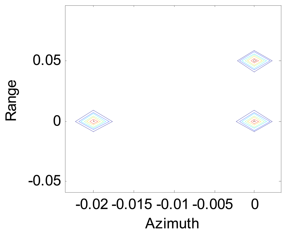
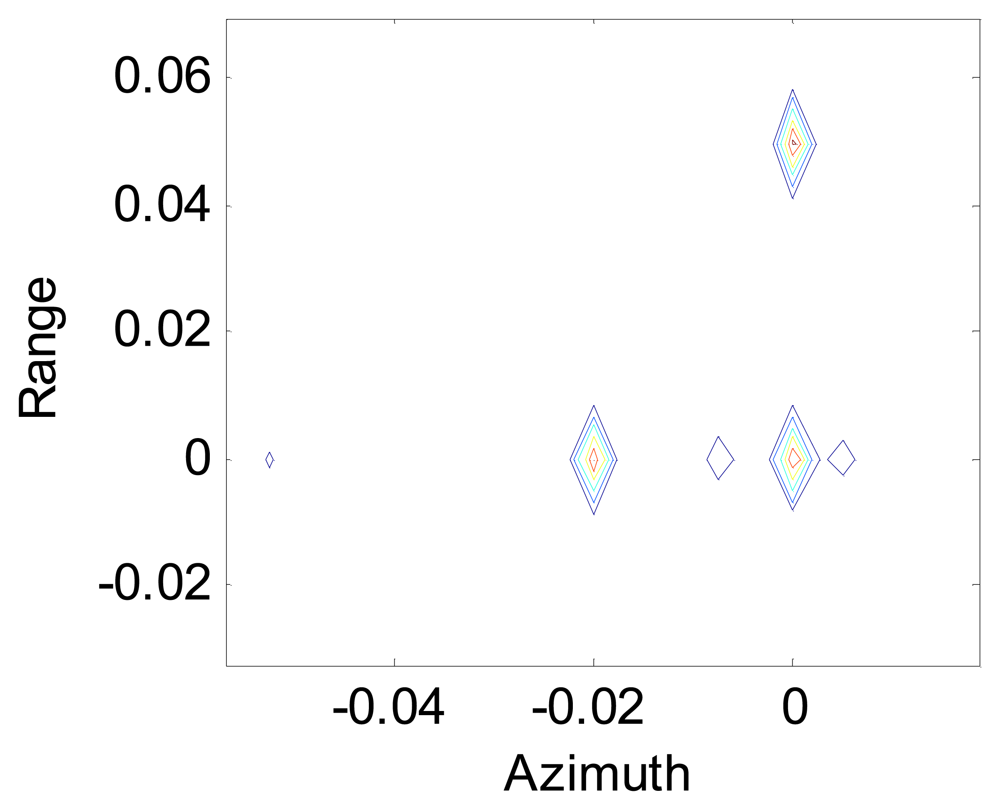
Figure 4 shows the image of a scene composed of three point objects, one at (0,0) m, one at (0.02,0) m and one at (0,0.05) m after SA processing using the modified Omega-K algorithm, and we can see that the points are all focused in range and azimuth.
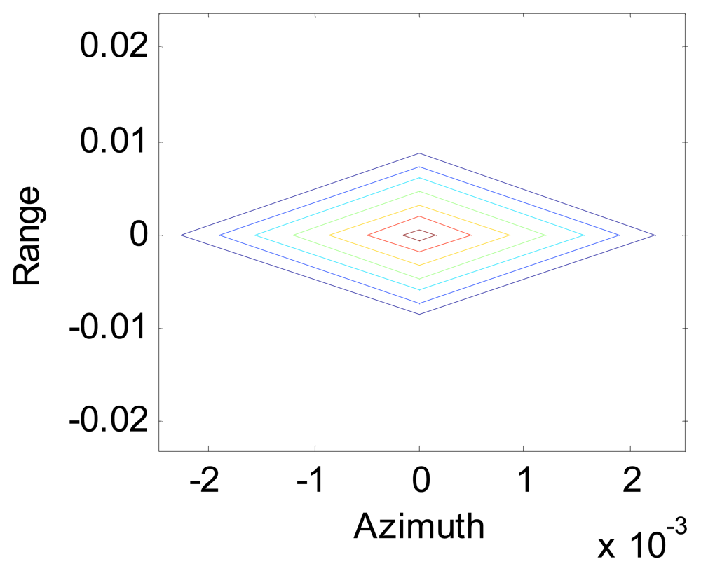
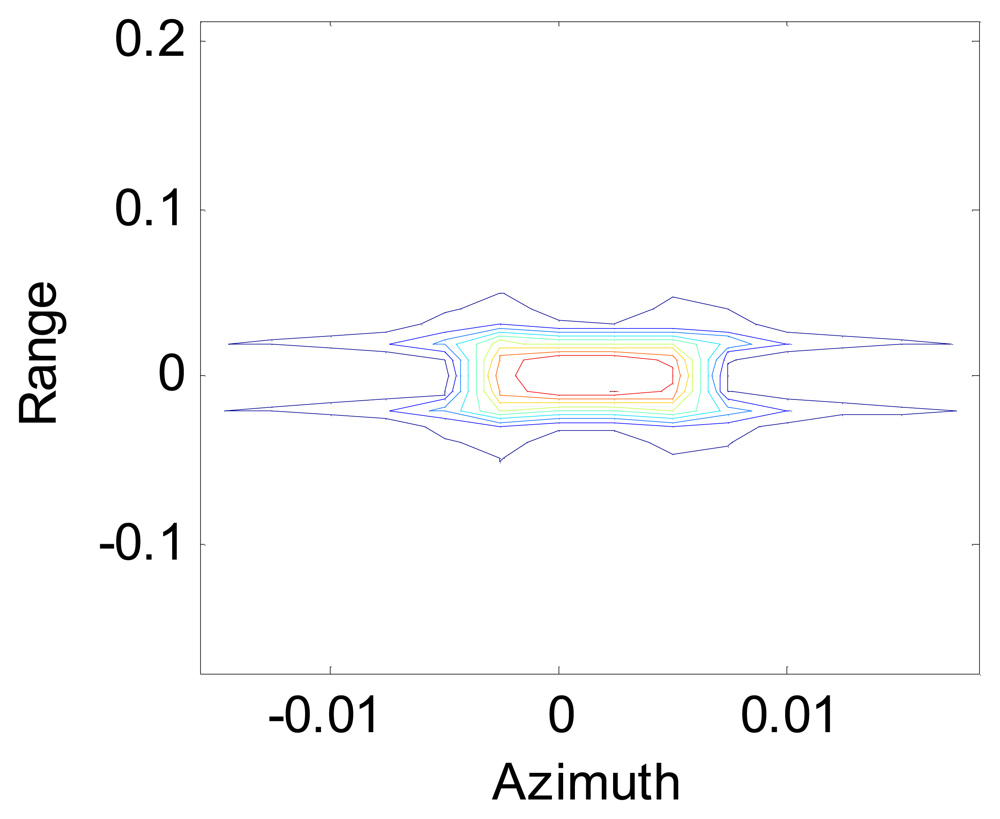
Figures 5 and
6 show the contour maps of a point after and before the Doppler shift compensation respectively.
Figure 5 shows the data processing after using the modified Omega-K algorithm, while
Figure 6 represents the data processing after using the conventional Omega-K algorithm. We can see that the data defocus if the Doppler shift induced by the continuous motion of the platform in the sweeps is not compensated.
Figure 7 shows the image of a scene composed of three point objects, one at (0,0) m, one at (0.02,0) m and one at (0,0.05) m, after SA processing for a fairly low level of turbulence, and it seems that there was no turbulence like
Figure 4. The loss of resolution is negligible when
r̃0 = 3.2
m for this case, while the length of the synthetic aperture is
LSA = 0.8
m.
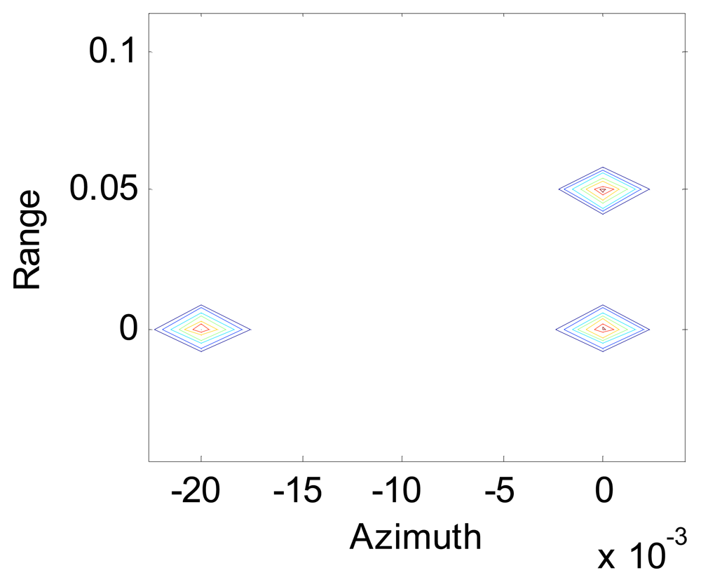
Figure 8 shows the image of the same scene with a little higher turbulence;
r̃0 = 1.6
m in this case and
LSA/
r̃0 = 1/2. The sidelobes become higher, and they come out pseudo-objects. But we can still recognize the point objects, and the resolution in range is unaffected.
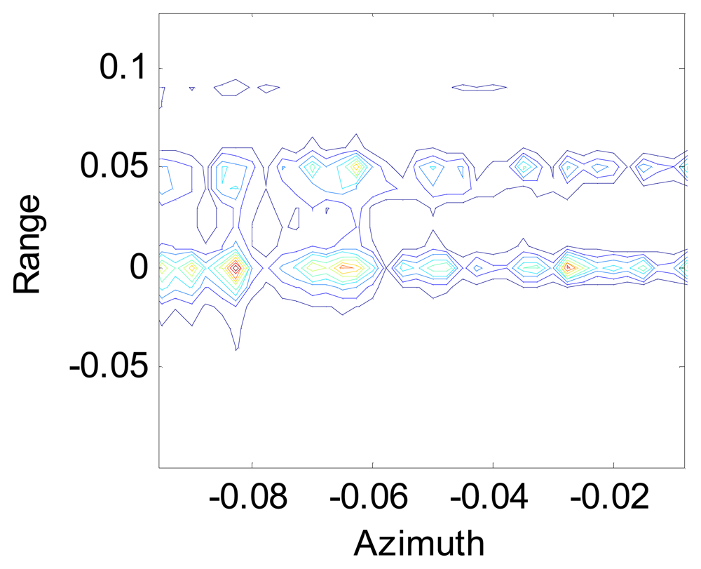
Figure 9 shows the image of the same scene with fairly high turbulence;
r̃0 = 0.1
m in this case and
LSA/
r̃0 = 8. We can see that image quality is severely degraded, but the resolution in range is also unaffected.


