1. Introduction
Currently, sensor networks are the main part of many monitoring and control systems. Many of them tend to be wireless because it allows them to be spatially distributed. Wireless Sensor Networks (WSNs) [
1] are formed dynamically because the connectivity between nodes depends on their position and their position variation over the time. These kinds of networks are easy to be deployed and are self-configuring. A sensor node is a transmitter, a receiver, and it offers services of routing between nodes without direct vision, as well as recording data from other sensors.
Since the 1950s, location systems have been incorporated into our lives. In the 1980s the Global Position System (GPS) [
2] began as a location method for outdoor environments. This system is based on a triangulation system of variables, where we know the position of a device thanks to the existing satellite network. Now, this system remains the most used because of its good performance and the low price of the required devices. At the end of the year 2000 other location systems appeared, based on cellular networks [
3]. These systems are designed for emergency situations. In this case, the base stations are used as a reference point and the location is made through the distance and the angle of the signal. These systems are developed to work in outdoor environments and the devices must also have several communication skills.
Previous technologies are not adequate for indoor environments. This is mainly due to the signal characteristics. Other wireless technologies, such as IEEE 802.11a/b/g [
4], Radio Frequency IDentification (RFID) [
5], Ultra Wide Band wideband (UWB) [
6], Bluetooth [
7] or Zigbee [
8], must be used for indoor locations. The main problem in these environments is the multipath effect and signal variability. The location in these types of environments can be centralized [
4] or distributed [
9]. The centralized location uses reference devices. These devices tend to have a greater capacity and they are located in a fixed position, for example a base station (BS) or an Access Point (AP). In contrast, in the distributed location there are no reference devices. The devices interact with their neighbors in order to know their position.
A study about the oscillation of the received signal is shown in reference [
10]. The RSS variation is introduced in our approach in order to obtain smaller degree errors in the location service. The three main issues that make variations in the RSS are the following ones:
Temporal variations: when the receiver remains in a fixed position, the signal level measured varies as time goes by.
Small-Scale variations: the signal level changes when the device is moving over small distances (less than the wavelength). In IEEE 802.11 b/g technologies the wavelength is 12.5 cm.
Large-Scale variations: the signal level varies with the distance due to the attenuation that the radio frequency (RF) signal suffers with the distance.
Besides these typical variations of the RF signal together with the receiver mobility, we have also considered the temperature and humidity variations, the effect of opening and closing doors, the changes in the localization of the furniture, and the presence and movement of human beings, which are all characteristics of indoor environments. These variations have already been analyzed in [
11].
All these systems can be used in different applications. Localization in sensor networks has attracted a large research effort in the last decade. Some WSNs location systems application areas are:
Emergencies: When we want to locate an individual in the case of an emergency (injury or criminal attacks) or in a life-threatening situation. Both can be located using the positioning capability of the mobile device.
Information: It can be used in public places such as swimming pools, museums, conferences, etc. in order to provide information service about this place to the user depending on his position.
Navigation: When the user needs to meet the situation of addresses, positions, directions in an indoor places such as big supermarkets, commercial centers, etc.
Discovery: When it is necessary to find or locate things or persons in indoor places. It is very useful to locate people with Alzheimer or to locate disabled people with very little motion.
Security: It can be used to avoid theft, to move unwanted items, etc. Wireless sensors would be in specific places, when the sensors transfer a position threshold they send an alarm.
Tracking: When it is required to track a device or person inside a building.
There are two main methods to estimate the position in indoor environments. On the one hand, there are the so-called deductive methods. These take into account the physical properties of signal propagation. They require a propagation model, topological information about the environment, and the exact position of the base stations. On the other hand, there are the so-called inductive methods. These require a previous training phase, where the system learns the signal strength in each location. The main shortcoming of this approach is that the training phase can be very expensive. The complex indoor environment makes the propagation model task very hard. It is difficult to improve deductive methods when there are many walls and obstacles because deductive methods work estimating the position mathematically with the real measures taken directly from environment in the training phase [
12].
In this work we present a hybrid location system using a new stochastic approach which is based on a combination of deductive and inductive methods. This system has been developed for wireless sensor networks using the IEEE 802.11b/g standard in order to use a deployed wireless access network that is also used for internet access and data transfer. On the other hand, the aforementioned technology allows us to cover a hard indoor environment without many base stations. The goal of this work is to reduce the training phase without losing precision.
The remainder of this paper is organized as follows. Section 2 presents the best known related work on location methods in sensor networks. Our hybrid location system is described in Section 3. Section 4 shows the efficiency of our system. It shows real measurements and compares our proposal with other systems. A comparison between our proposal and other hybrid systems proposed in the literature is shown in Section 5. Section 6 concludes the paper and discloses our planned future work.
3. Hybrid Stochastic Approach to Location Estimation
In this section we explain the mathematical assumptions used in our proposal. We analyse the inductive and deductive methods from a statistical point of view. In this way, we can describe our hybrid model.
Table 1 shows the variables used in the analysis.
3.1. Stochastic Approach for Location Estimation
The location estimation problem can be statistically stated as follows. For simplicity, the true distribution Pr(X = x) and Pr(X = x | Y = y) are denoted as Pr(x) and Pr(y). The model parameters are denoted by p( ).
Let b be the number of base-stations. We denote o as an observation. The observation variable is a b-dimensional vector; one for each signal strength from each base-station. We denote as oj the signal strength from base-station j for j ∈ {1,…,b}. We have a location l associated to each observation. In this work we use bi-dimensional locations for simplicity, but it can be used in three dimensions easily.
The methodology used is based on the definition of a function Pr(
l|
o) that returns the probability of the location
l, given the observation
o. This nomenclature has been used in other proposals [
22,
28,
29]. Once this function is estimated, the problem can be formulated to find the location
l that maximizes the probability Pr(
l|
o) for a given observation
o. Using Bayes' theorem, we can write:
The denominator in
equation (1) does not depend on the location variable
l. And, therefore, the location estimation problem can be presented as:
where Pr(
l) is the
prior probability of the location
l, knowing the observation. This probability can be used to incorporate information such a more training locations [
22] or tracking [
29] to our statistical model. The tracking information will not be taken into account in this work, so, for the prior probability, we use the uniform distribution.
In
equation (1), Pr(
o|
l) is the so called
likelihood function. It estimates the probability of one observation given a location. In the literature, we find two main approaches to estimate this function: inductive approach and deductive approach. The next two subsections explain these methods analytically in order to propose our approach.
3.2. Inductive Approach for Location Estimation
On the one hand, the
inductive approach estimates the
likelihood function measuring directly the signal strength in each place. That is, several measurements are taken for each training place; then, the function p(
o|
l) is estimated. The main drawback of this approach is the time consuming nature of the training phase. We denote as
T the set of training data, formed by
t observations with their respective locations. Each training data,
Ti, it is represented as (
li,
oi), where
i can be from 1 to
t. Several alternatives has been proposed in the literature to estimate p(
o|
l) from
T: the histogram method [
30,
32], the Bayesian method [
33] or the kernel method [
30,
34]. Another drawback is that this model only returns one of the locations from the training set. In order to solve this problem, several proposals can be found in reference [
35].
3.3. Deductive Approach for Location Estimation
On the other hand, the
deductive approach estimates the
likelihood function by using empirical formulas about the signal propagation in an indoor environment. In this approach, we need to know the location of each base-station, the described map of the environment (walls, obstacles, etc.) and a propagation model. Several propagation models can be seen in references [
35,
36]
If we assume that each observation
oj, from the vector o, is mutually independent, we can write:
where
b is the number of base-stations;
Bj is the base-station
j; and,
oj is the observation signal strength from base-station
j. In our study the base-station
Bj is characterized by two variables (
lj,
o0j). The variable
lj denotes the location of base-station
j, and o
0j denotes the mean signal strength measured to
d0 distance from base-station
j.
In this work, we assume that (
oj|
l,Bj) follows a Gaussian distribution with standard derivation σ. The following empirical propagation model, which supposes that signal strength is measured in dB, is used [
36,
37]:
where,
dj is the Euclidian distance between the observation location (
l) and the base-station
j (
lj),
n is the attenuation variation index (
n value depends on the specific propagation environment) and
Lwj is the attenuation caused by the obstacles. In our study the value of
Lwj depends on the number of walls that the line of sight crosses from the base-station
j to the location. We will use
Lwj =
wL0. Where
w is the number of wall crossed and
L0 is the wall average attenuation. Finally, let
N(
μ,
σ2) be the normal distribution with mean
μ and variance
σ2.
3.4. Stochastic Hybrid Approach for Location Estimation
In the inductive approach we assume that the signal distribution for each training sample location is known in advance. Taking a sample for all possible locations is not a realistic assumption. However, for a given location we can have several training samples near to our location. In the hybrid approach we are interested in combining the information of both previous approaches to improve the system. That is, we know the signal distribution for several training samples near our location and we know how the signal is attenuated from the location of these samples to our actual location. Without loss of generality, we can write:
We assume that Pr(
Ti|
l) is uniformly distributed. Then, we are only interested in defining the second term. Using the same assumption that in
equation (3), we can write:
Now, we define the random variable (
oj|
l,Bj,T
i) in the same manner as (
oj|
l,Bj) has been defined in
equation (4). But, instead of
o0j (the signal strength measured in the reference distance
d0), we use
oij (the signal strength measured in the training sample location
i).
where
oij is a random variable that represent the signal strength of training sample
i from base-station
j. dij is the distance from training sample
i to the base station
j. And,
Lwij is the wall attenuation from training sample
i to the base station
j. Note that in this equation,
Xσ has been eliminated because the variability is included in the random variable
oij.
3.5. Implementation Details
From
equation (7) the random variable
oij can be expressed as follows:
In the training phase, we have estimated p(
oij |
li,Bj). In this stage several methods such as histogram or kernel can be used. Then, using
equation (8), we can write:
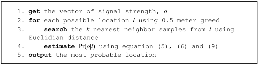
where n = 2 in free space. In order to obtain the optimal location for
equation (2), the proposed algorithm is written in pseudocode in
Figure 1. Its explanation is as follows: given the input signal strength the location probability for each point is evaluate using 0.5 meter greed. For each point the k nearest samples are taken. The probability of this location is calculated using
equation (5), but, using only these k samples instead the all training set. Farther samples will distort the results. For each sample (of k nearest samples), first we use
equation (9) to combine the deductive approach, to take into account the shift from the actual location to the sample location, and, second the inductive approach, to obtain the signal probability in a well known place.
4. Experimental Results
This section shows the results obtained from a real environment to test our proposal. First, we will test the errors based on the number of samples and based on the number of base stations. Then, we compare it with other commercial and implemented location systems.
4.1. Test Bench
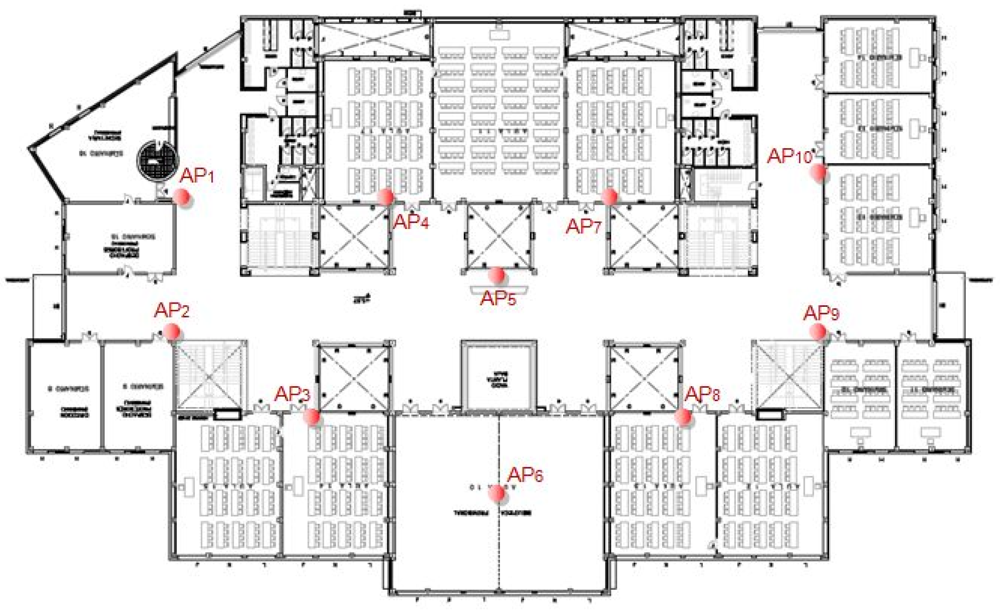
To assess our proposal, we have deployed the approach in an indoor wireless environment. This place is located on the first floor of the “A building” in the “Campus Gandia” of the Polytechnic University of Valencia. The distribution of this floor is shown in
Figure 2. There are 10 access points acting as base stations. These base stations have a fixed position and their transmission power is known in advance.
4.2. Error Measurement Based on the Number of Samples
Our proposal takes into account k nearest neighbour samples from a position using Euclidian distance (see
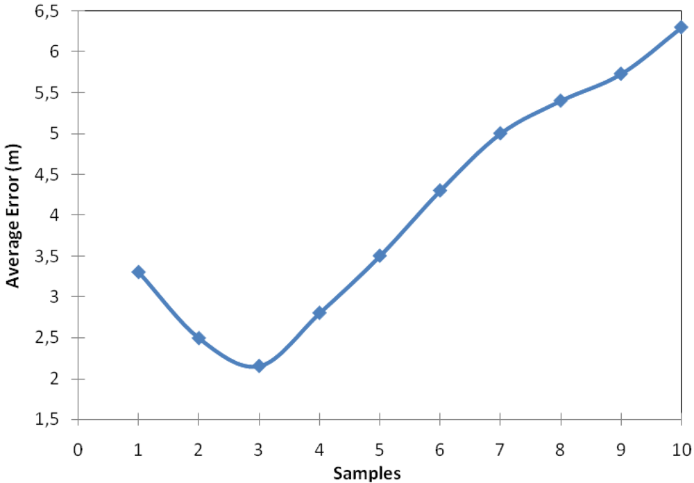
Figure 1). This experiment gives us the optimum number of samples in order to obtain the lowest error. In order to test our approach we took 56 samples spread equitably throughout the floor of the building. The floor was split in a grid where sampling points are placed every 2 meters.
Figure 3 shows that the error is not reduced linearly as regards the number of samples. It has an inflection point in which the error changes its trend. In other words, the error decreases until it has the three closest samples, then, the error begins to increase.
This happens because the method obtains relative distances from the samples to the sensor and when the method begins to use measures that are not close to the sensor the error increases. Obviously, the smaller the area is, where the sensor can be found, the lower the error in its location will be. More samples will give higher relative distances and therefore the error of location will be greater.
Our first conclusion, based on the previous graph, is that given a fixed number of samples, there will be a value of number of samples where the location error will be the optimal. Then, if the number of samples used to train the system is greater, the estimated position will be more accurate because there will be closer samples.
4.3. Error Measurement Based on the number of APs (Base Stations)
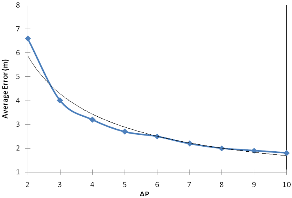
In order to test the influence of the number of APs in our proposal, we measured the error of the approach adding access point one by one in each location (in the same place of the 56 samples previously taken). In
Figure 4 we can observe that the localization error tends to decrease exponentially (blue line with squares). Therefore, with higher number of APs we obtain lower error values in the sensor location estimation. This tendency is given because one of the methods used in our hybrid system is based on the triangulation method. This method uses the distance from the sensor to various access points based on RSS. Once the sensor obtains the value of at least three distances, between the sensor and the APs, the sensor estimates its position. Therefore, the more distances the sensor to different APs has, the higher the accuracy of the localization sensor will be, in other words, the error of location will be lower.
Bearing in mind this tendency, we have estimated which function follows the error when the number of APs of the indoor environment varies.
Equation (10) gives our estimation:
where
x is the number of APs in the indoor environment.
Equation (10) is shown in
figure 4 with the black-thin line. We can see that it fits the error tend quite well.
It should be noted, that when there are more than five APs the improvement appreciation in terms localization error is minimal when a new AP is added to the indoor environment.
4.4. Comparative Measurement with others Existing Location Systems
In order to compare our proposal with others, we have evaluated five wireless sensor location systems:
Inductive 1. This is an inductive location system which has enough a number of samples for an adequate training.
Inductive 2. It is also an inductive location system, but in this case, the number of samples is very low.
Deductive. This system uses the method based on the equation of spread that we have seen in subsection 4.3.
The Hybrid method. This is our proposed method.
Ekahau, which is the basis of many currently used location systems [
38].
For the inductive methods we used a system described in our previous work [
11]. As has been previously mentioned, inductive methods need a training phase. For the Inductive 1 and Ekahau methods, we collected 312 samples spread equitably throughout the floor of the building. The floor was split in a grid where sampling points are placed every 2 meters. Thirty observations were taken from each training point; 15 of them were taken one day and the other 15 were taken one week later. In contrast, for the Inductive 2 and hybrid methods we used a subset of 56 samples. For the hybrid method we estimated p(
oi|
l) using the histogram method shown in references [
30,
32].
In the test phase, all these systems were tested for 40 locations (all these locations were different that the training ones, they were randomly placed and they were not inside the training grid). For each location we gathered a mean of 15 RSS consecutive values. This let us take into account the signal variability in the measurements. Each one of the test samples has been applied to the different location methods. Then, we estimate the error measuring the Euclidean distance between the output of the method and the real location of the sample.
Figure 5 shows the results obtained for all the location systems as a function of the number of APs. Their graph follows an exponential tends approximately.
We note that the Inductive 2 method has a higher localization error than the others. This method had 56 training samples. They were few compared with the Inductive 1 method (312 samples). This difference gives considerably more accuracy in the Inductive 1 than the Inductive 2 method.
With regards to the deductive model, we note that it did not give good results because the floor where the measurements were taken had many walls, so there was very little accuracy when we estimated their loss.
The hybrid model proposed in this paper has a stable and optimal graph compared to the rest of systems (with few training measures low errors were obtained). As noted in
Figure 5, for a certain number of AP (five APs) its average error remains the second best.
Finally, the Ekahau system together with the Inductive 2 system are the methods with the worst results.
In
Table 2 we can see the average error and the standard deviation of the approached compared in our experiment. We see that the method with less error is the Inductive 1 (1.23 m), this is because the number of samples is adequate. The model with the worst behaviour is the Inductive 2 (3.02 m). The proposed hybrid method has an average error of 1.80 m, with the advantage that training is minimal. A statistical significance test has been calculated using a paired t-test (the hybrid approach is used as reference). A result labelled with a “
▲”means statistical confidence of 99%. “
Δ” means statistical confidence of 90%.
5. Hybrids Methods Comparison
This section compares our proposal with the hybrid methods found in the literature. In
Table 3 we can see the performance analysis. First, we analyzed the analytical techniques used. All cases use multiple parameters, except in [
28,
29] and our proposal. The next feature compared was their working environment (indoor or outdoor environments). Our proposal and the one in reference [
28] support both environments. The systems used in WSNs are [
26,
27] and our application; the others are used for other purposes. Our location system has a better accuracy (1.8 m) than other works, although the systems in [27, 28 and 29] have good features too.
The next analyzed feature is the number of stages to ascertain the final position. In this case, our system has two stages. The best solution is one stage because of simplicity. As we can see in
Table 3, only the systems in [
26] and [
27] have one stage, but these systems need extra messages to estimate the location. But, on the other hand there are several works that demonstrate that sending messages wastes more energy than computing [
39]. Finally we have analyzed the centralization and decentralization of the location systems and if they are recursively updated. Only our proposal and the one in reference [
28] are recursively updated. In conclusion, we can see that the proposed location system has more positive features and it improves all analyzed hybrid location systems.
6. Conclusions
In this paper two different approaches had been discussed. The so-called deductive methods, which require a model of propagation, a topological information of the environment, and the exact position of the radio stations, and the so-called inductive methods, which require a previous training phase where the system learns the signal strength in each location. The main shortcoming of this approach is that in some scenarios, the training phase cannot be done or could be very expensive. On the other hand, the Euclidean models are optimum when there are multiple access points and few walls.
In this work we present a hybrid location system using a new stochastic approach which is based on a combination of deductive and inductive methods. This system has been developed for wireless sensor networks using IEEE 802.11b/g standard in order to use a deployed wireless access network that is also used for internet access and data transfer.
We have tested the errors based on the number of samples and based on the number of base stations. We have estimated an experimental equation based on the graph trends of the errors of the measures obtained. We have compared our proposal with several methods in order to check our approach.
Our system uses a small set of training samples (inductive information). Given the actual signal strength, we use the closest training samples as a starting point. Then, the deductive propagation model is used to obtain the shift from the training samples. A stochastic approach is used whereby the optimal location can be estimated as the point that maximizes the product of probabilities from each of the closest training samples
Our proposal combines the advantages of the deductive and inductive methods in order to provide accurate measurements in hard environments (few base stations and/or few trained points). The goal of this work has been to reduce the training phase without losing precision. Now, we are trying to find the proposed model by adding other methods in order to obtain more accurate results.
The proposed method is useful in cases where a good training phase is not practical (very few samples can be taken in advance), and the precise location of some access points is not known. These environments could be military, such as troop deployments inside buildings or discovery squads for hard environments, environments where the radio coverage is not known in advance (unknown deployments), or even environments where there the APs can be on or off at any time (dynamic environments). We are currently working on enhancing the precision of the proposed model. In future work we will evaluate the performance our proposal in hard environments.


