Sensitivity Improvement and Determination of Rydberg Atom-Based Microwave Sensor


Abstract
:1. Introduction
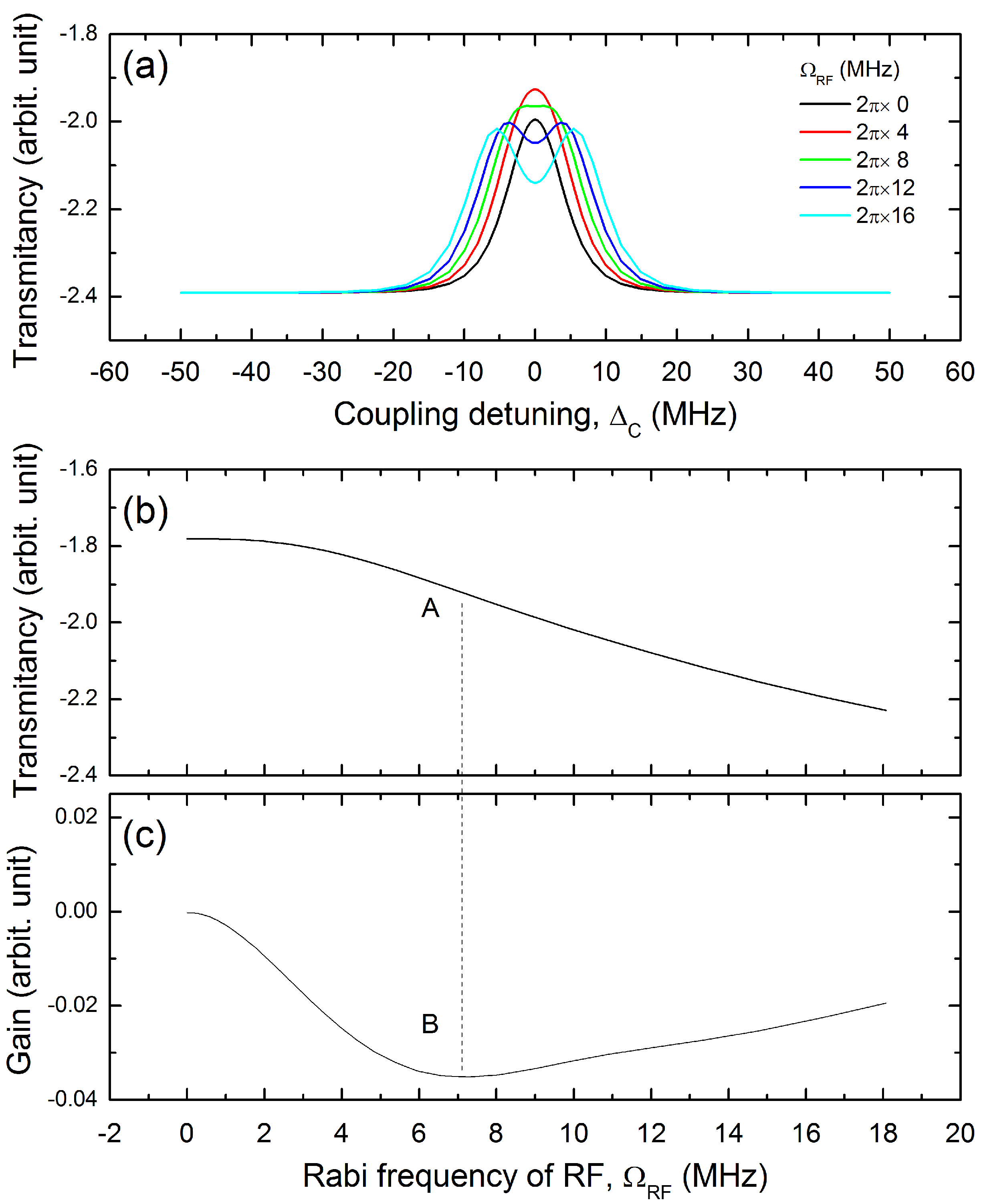
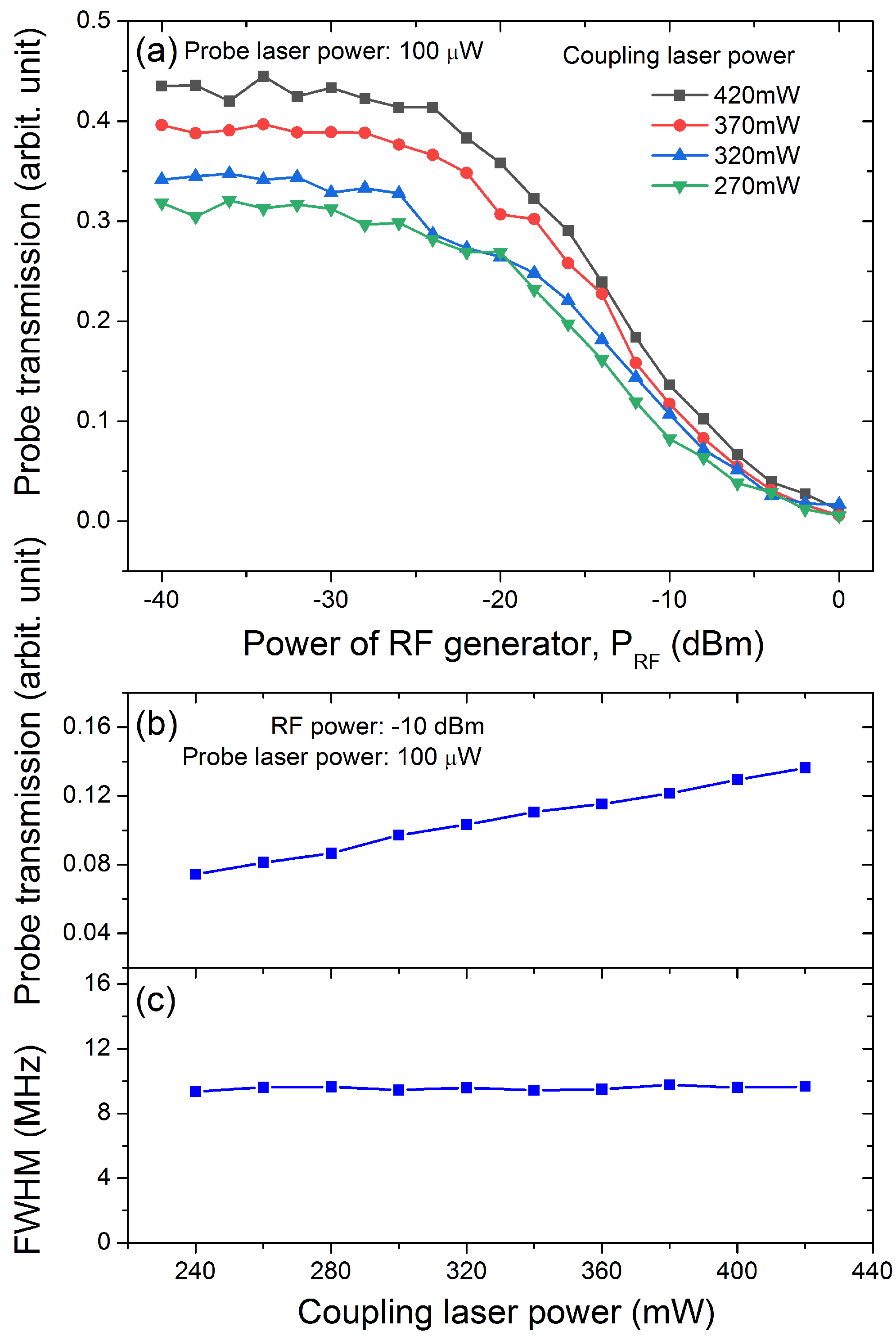
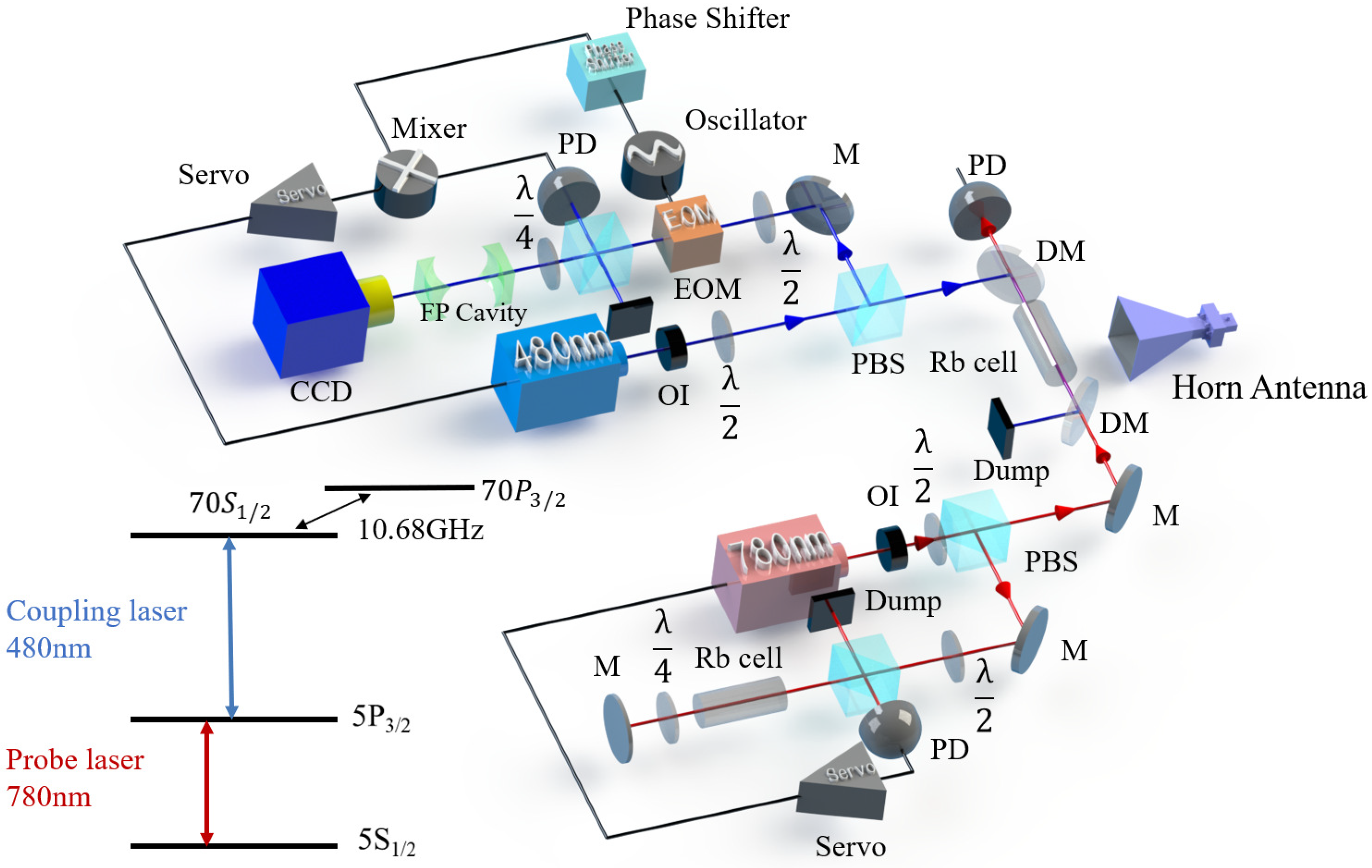
2. Theory and Experimental Setup
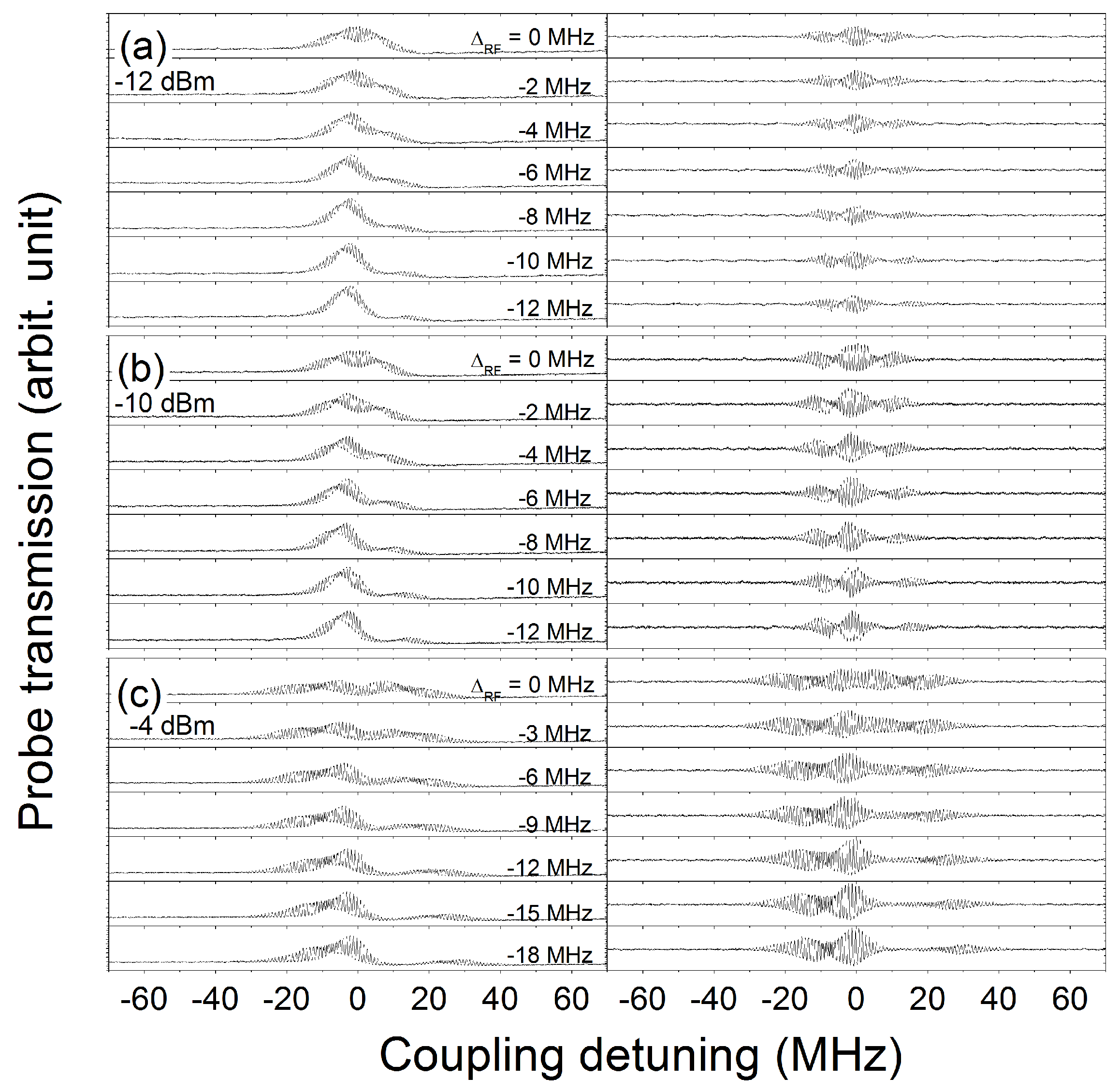
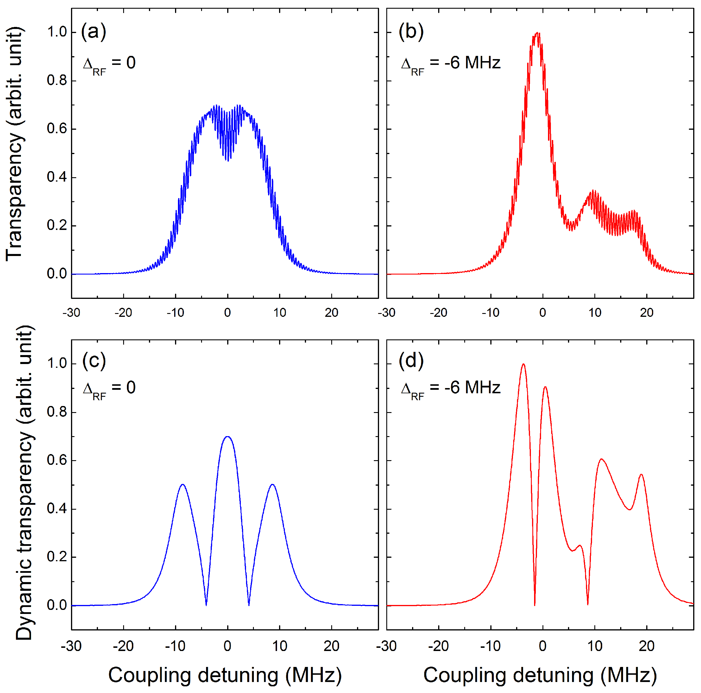
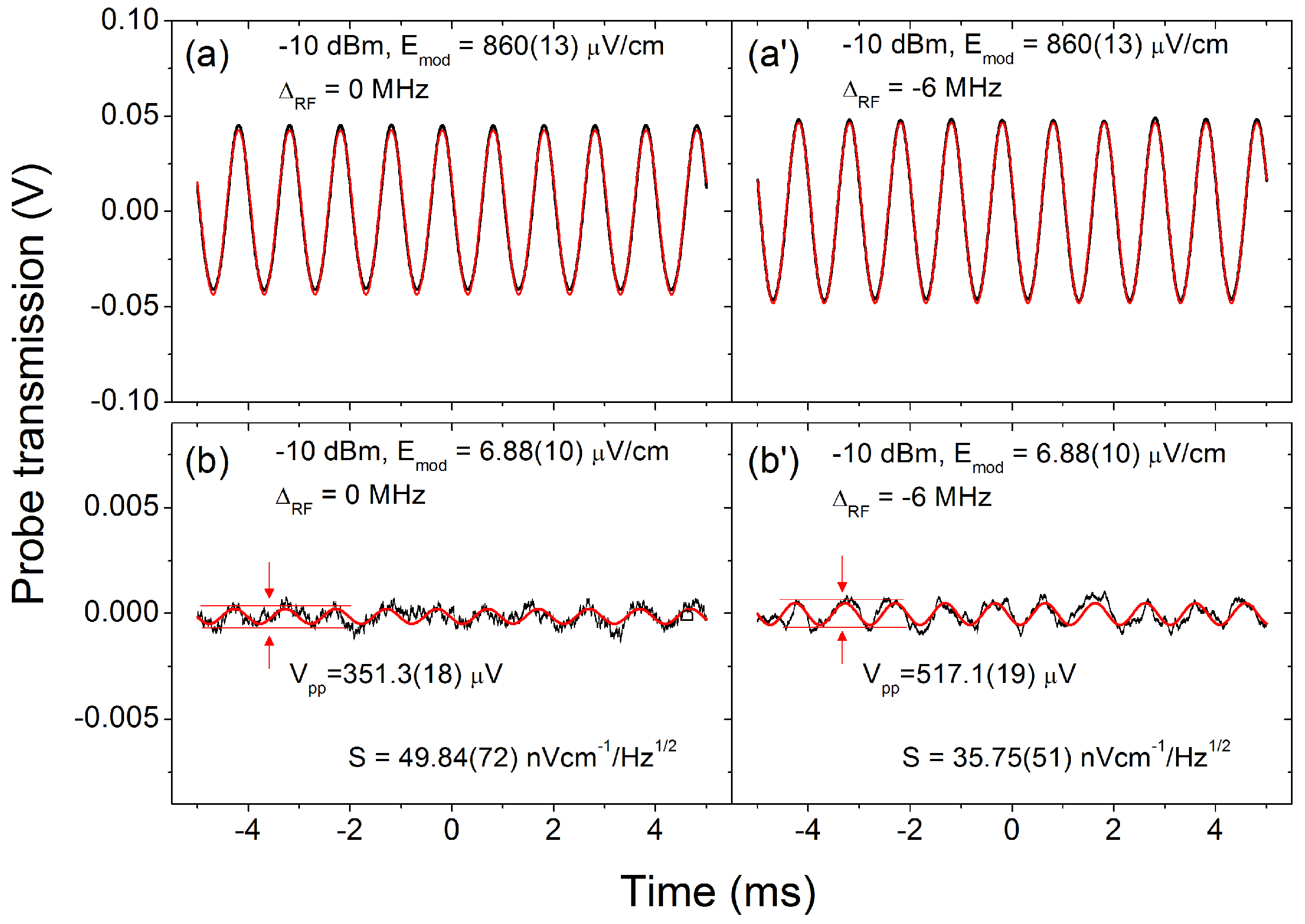
3. Results
4. Conclusions
Author Contributions
Funding
Institutional Review Board Statement
Informed Consent Statement
Data Availability Statement
Conflicts of Interest
References
- Gallagher, T.F.; Safinya, K.A.; Gounand, F.; Delpech, J.F.; Sandner, W.; Kachru, R. Resonant Rydberg-atom—Rydberg-atom collisions. Phys. Rev. A 1982, 25, 1905–1917. [Google Scholar] [CrossRef]
- Deb, A.B.; Kjærgaard, N. Radio-over-fiber using an optical antenna based on Rydberg states of atoms. Appl. Phys. Lett. 2018, 112, 211106. [Google Scholar] [CrossRef]
- Holloway, C.L.; Simons, M.T.; Kautz, M.D.; Haddab, A.H.; Gordon, J.A.; Crowley, T.P. A quantum-based power standard: Using Rydberg atoms for a SI-traceable radio-frequency power measurement technique in rectangular waveguides. Appl. Phys. Lett. 2018, 113, 094101. [Google Scholar] [CrossRef]
- Sedlacek, J.A.; Schwettmann, A.; Kübler, H.; Löw, R.; Pfau, T.; Shaffer, J.P. Microwave electrometry with Rydberg atoms in a vapour cell using bright atomic resonances. Nat. Phys. 2012, 8, 819–824. [Google Scholar] [CrossRef]
- Simons, M.T.; Gordon, J.A.; Holloway, C.L. Fiber-coupled vapor cell for a portable Rydberg atom-based radio frequency electric field sensor. Appl. Opt. 2018, 57, 6456–6460. [Google Scholar] [CrossRef]
- Simons, M.T.; Haddab, A.H.; Gordon, J.A.; Holloway, C.L. Applications with a Rydberg Atom-based Radio Frequency Antenna/Receiver. In Proceedings of the 2019 International Symposium on Electromagnetic Compatibility—EMC EUROPE, Barcelona, Spain, 2–6 September 2019; pp. 885–889. [Google Scholar]
- Song, Z.; Liu, H.; Liu, X.; Zhang, W.; Zou, H.; Zhang, J.; Qu, J. Rydberg-atom-based digital communication using a continuously tunable radio-frequency carrier. Opt. Express 2019, 27, 8848–8857. [Google Scholar] [CrossRef] [Green Version]
- Liao, K.Y.; Tu, H.T.; Yang, S.Z.; Chen, C.J.; Liu, X.H.; Liang, J.; Zhang, X.D.; Yan, H.; Zhu, S.L. Microwave electrometry via electromagnetically induced absorption in cold Rydberg atoms. Phys. Rev. A 2020, 101, 053432. [Google Scholar] [CrossRef]
- Zhang, L.; Jia, Y.; Jing, M.; Guo, L.; Zhang, H.; Xiao, L.; Jia, S. Detuning radio-frequency electrometry using Rydberg atoms in a room-temperature vapor cell. Laser Phys. 2019, 29, 035701. [Google Scholar] [CrossRef]
- Jia, F.D.; Liu, X.B.; Mei, J.; Yu, Y.H.; Zhang, H.Y.; Lin, Z.Q.; Dong, H.Y.; Zhang, J.; Xie, F.; Zhong, Z.P. Span shift and extension of quantum microwave electrometry with Rydberg atoms dressed by an auxiliary microwave field. Phys. Rev. A 2021, 103, 063113. [Google Scholar] [CrossRef]
- Simons, M.T.; Artusio-Glimpse, A.B.; Holloway, C.L.; Imhof, E.; Jefferts, S.R.; Wyllie, R.; Sawyer, B.C.; Walker, T.G. Continuous radio-frequency electric-field detection through adjacent Rydberg resonance tuning. Phys. Rev. A 2021, 104, 032824. [Google Scholar] [CrossRef]
- Meyer, D.H.; Kunz, P.D.; Cox, K.C. Waveguide-Coupled Rydberg Spectrum Analyzer from 0 to 20 GHz. Phys. Rev. Appl. 2021, 15, 014047. [Google Scholar] [CrossRef]
- Peng, Y.D.; Wang, J.L.; Li, C.; Lu, X.; Qi, Y.H.; Yang, A.H.; Wang, J.Y. Enhanced microwave electrometry with intracavity anomalous dispersion in Rydberg atoms. Opt. Quantum Electron. 2020, 52, 120. [Google Scholar] [CrossRef]
- Holloway, C.L.; Gordon, J.A.; Jefferts, S.; Schwarzkopf, A.; Anderson, D.A.; Miller, S.A.; Thaicharoen, N.; Raithel, G. Broadband Rydberg Atom-Based Electric-Field Probe for SI-Traceable, Self-Calibrated Measurements. IEEE Trans. Antenna Propag. 2014, 62, 6169–6182. [Google Scholar] [CrossRef] [Green Version]
- Simons, M.T.; Haddab, A.H.; Gordon, J.A.; Novotny, D.; Holloway, C.L. Embedding a Rydberg Atom-Based Sensor Into an Antenna for Phase and Amplitude Detection of Radio-Frequency Fields and Modulated Signals. IEEE Access 2019, 7, 164975–164985. [Google Scholar] [CrossRef]
- Fan, H.Q.; Kumar, S.; Daschner, R.; Kubler, H.; Shaffer, J.P. Subwavelength microwave electric-field imaging using Rydberg atoms inside atomic vapor cells. Opt. Lett. 2014, 39, 3030–3033. [Google Scholar] [CrossRef] [Green Version]
- Gordon, J.A.; Holloway, C.L.; Schwarzkopf, A.; Anderson, D.A.; Miller, S.; Thaicharoen, N.; Raithel, G. Millimeter wave detection via Autler-Townes splitting in rubidium Rydberg atoms. Appl. Phys. Lett. 2014, 105, 024104. [Google Scholar] [CrossRef] [Green Version]
- Holloway, C.L.; Gordon, J.A.; Schwarzkopf, A.; Anderson, D.A.; Miller, S.A.; Thaicharoen, N.; Raithel, G. Sub-wavelength imaging and field mapping via electromagnetically induced transparency and Autler-Townes splitting in Rydberg atoms. Appl. Phys. Lett. 2014, 104, 244102. [Google Scholar] [CrossRef] [Green Version]
- Sedlacek, J.A.; Schwettmann, A.; Kubler, H.; Shaffer, J.P. Atom-based vector microwave electrometry using rubidium Rydberg atoms in a vapor cell. Phys. Rev. Lett. 2013, 111, 063001. [Google Scholar] [CrossRef] [Green Version]
- Simons, M.T.; Gordon, J.A.; Holloway, C.L.; Anderson, D.A.; Miller, S.A.; Raithel, G. Using frequency detuning to improve the sensitivity of electric field measurements via electromagnetically induced transparency and Autler-Townes splitting in Rydberg atoms. Appl. Phys. Lett. 2016, 108, 174101. [Google Scholar] [CrossRef] [Green Version]
- Fan, H.; Kumar, S.; Sedlacek, J.; Kübler, H.; Karimkashi, S.; Shaffer, J.P. Atom based RF electric field sensing. J. Phys. B At. Mol. Opt. Phys. 2015, 48, 202001. [Google Scholar] [CrossRef]
- Jing, M.; Hu, Y.; Ma, J.; Zhang, H.; Zhang, L.; Xiao, L.; Jia, S. Atomic superheterodyne receiver based on microwave-dressed Rydberg spectroscopy. Nat. Phys. 2020, 16, 911–915. [Google Scholar] [CrossRef]
- Anderson, D.A.; Sapiro, R.E.; Raithel, G. An Atomic Receiver for AM and FM Radio Communication. IEEE Trans. Antenna Propag. 2021, 69, 2455–2462. [Google Scholar] [CrossRef] [Green Version]
- Holloway, C.; Simons, M.; Haddab, A.H.; Gordon, J.A.; Anderson, D.A.; Raithel, G.; Voran, S. A Multiple-Band Rydberg Atom-Based Receiver: AM/FM Stereo Reception. IEEE Antenna Propag. Mag. 2021, 63, 63–76. [Google Scholar] [CrossRef]
- Song, Z.; Zhang, W.; Liu, X.; Zou, H.; Zhang, J.; Jiang, Z.; Qu, J. Quantum-Based Amplitude Modulation Radio Receiver Using Rydberg Atoms. In Proceedings of the 2018 IEEE Globecom Workshops, Abu Dhabi, United Arab Emirates, 9–13 December 2018; pp. 1–6. [Google Scholar]
- Abi-Salloum, T.Y. Electromagnetically induced transparency and Autler-Townes splitting: Two similar but distinct phenomena in two categories of three-level atomic systems. Phys. Rev. A 2010, 81, 053836. [Google Scholar] [CrossRef]
- Petrosyan, D.; Otterbach, J.; Fleischhauer, M. Electromagnetically induced transparency with Rydberg atoms. Phys. Rev. Lett. 2011, 107, 213601. [Google Scholar] [CrossRef] [PubMed]
- Simons, M.T.; Haddab, A.H.; Gordon, J.A.; Holloway, C.L. Waveguide-integrated Rydberg Atom-based RF Field Detector for Near-field Antenna Measurements. In Proceedings of the 2019 Antenna Measurement Techniques Association Symposium, San Diego, CA, USA, 6–11 October 2019; pp. 1–4. [Google Scholar]
- Holloway, C.L.; Simons, M.T.; Gordon, J.A.; Dienstfrey, A.; Anderson, D.A.; Raithel, G. Electric field metrology for SI traceability: Systematic measurement uncertainties in electromagnetically induced transparency in atomic vapor. J. Appl. Phys. 2017, 121, 233106. [Google Scholar] [CrossRef] [Green Version]
- Kumar, S.; Fan, H.; Kubler, H.; Sheng, J.; Shaffer, J.P. Atom-Based Sensing of Weak Radio Frequency Electric Fields Using Homodyne Readout. Sci. Rep. 2017, 7, 42981. [Google Scholar] [CrossRef]
- Zou, H.; Song, Z.; Mu, H.; Feng, Z.; Qu, J.; Wang, Q. Atomic Receiver by Utilizing Multiple Radio-Frequency Coupling at Rydberg States of Rubidium. Appl. Sci. 2020, 10, 1346. [Google Scholar] [CrossRef] [Green Version]
- Valente, P.; Failache, H.; Lezama, A. Temporal buildup of electromagnetically induced transparency and absorption resonances in degenerate two-level transitions. Phys. Rev. A 2003, 67, 013806. [Google Scholar] [CrossRef] [Green Version]
- Li, Y.Q.; Xiao, M. Transient properties of an electromagnetically induced transparency in three-level atoms. Opt. Lett. 1995, 20, 1489–1491. [Google Scholar] [CrossRef]
- Zi-Shan, X.; Han-Mu, W.; Zeng-Li, B.; Hong-Ping, L. Transient electromagnetically induced transparency spectroscopy of 87Rb atom in buffer gas. Chin. Phys. B 2021. [Google Scholar] [CrossRef]
- Gea-Banacloche, J.; Li, Y.; Jin, S.; Xiao, M. Electromagnetically induced transparency in ladder-type inhomogeneously broadened media: Theory and experiment. Phys. Rev. A 1995, 51, 576–584. [Google Scholar] [CrossRef] [PubMed]
- Sibalic, N.; Pritchard, J.D.; Adams, C.S.; Weatherill, K.J. ARC: An open-source library for calculating properties of alkali Rydberg atoms. Comput. Phys. Commun. 2017, 220, 319–331. [Google Scholar] [CrossRef]
- Liu, X.; Jia, F.; Zhang, H.; Mei, J.; Yu, Y.; Liang, W.; Zhang, J.; Xie, F.; Zhong, Z. Using amplitude modulation of the microwave field to improve the sensitivity of Rydberg-atom based microwave electrometry. AIP Adv. 2021, 11, 085127. [Google Scholar] [CrossRef]
- Chopinaud, A.; Pritchard, J.D. Optimal State Choice for Rydberg-Atom Microwave Sensors. Phys. Rev. Appl. 2021, 16, 024008. [Google Scholar] [CrossRef]
- Robinson, A.K.; Artusio-Glimpse, A.B.; Simons, M.T.; Holloway, C.L. Atomic spectra in a six-level scheme for electromagnetically induced transparency and Autler-Townes splitting in Rydberg atoms. Phys. Rev. A 2021, 103, 023704. [Google Scholar] [CrossRef]


Publisher’s Note: MDPI stays neutral with regard to jurisdictional claims in published maps and institutional affiliations. |
© 2022 by the authors. Licensee MDPI, Basel, Switzerland. This article is an open access article distributed under the terms and conditions of the Creative Commons Attribution (CC BY) license (https://creativecommons.org/licenses/by/4.0/).
Share and Cite
Cai, M.; Xu, Z.; You, S.; Liu, H. Sensitivity Improvement and Determination of Rydberg Atom-Based Microwave Sensor. Photonics 2022, 9, 250. https://doi.org/10.3390/photonics9040250
Cai M, Xu Z, You S, Liu H. Sensitivity Improvement and Determination of Rydberg Atom-Based Microwave Sensor. Photonics. 2022; 9(4):250. https://doi.org/10.3390/photonics9040250
Chicago/Turabian StyleCai, Minghao, Zishan Xu, Shuhang You, and Hongping Liu. 2022. "Sensitivity Improvement and Determination of Rydberg Atom-Based Microwave Sensor" Photonics 9, no. 4: 250. https://doi.org/10.3390/photonics9040250
APA StyleCai, M., Xu, Z., You, S., & Liu, H. (2022). Sensitivity Improvement and Determination of Rydberg Atom-Based Microwave Sensor. Photonics, 9(4), 250. https://doi.org/10.3390/photonics9040250