
Numerical Investigation of T-Shaped Microfluidic Oscillator with Viscoelastic Fluid

 ,
, 


Abstract
:1. Introduction
2. Numerical Procedure
2.1. Physical Model
2.2. Governing Equations and Numerical Method
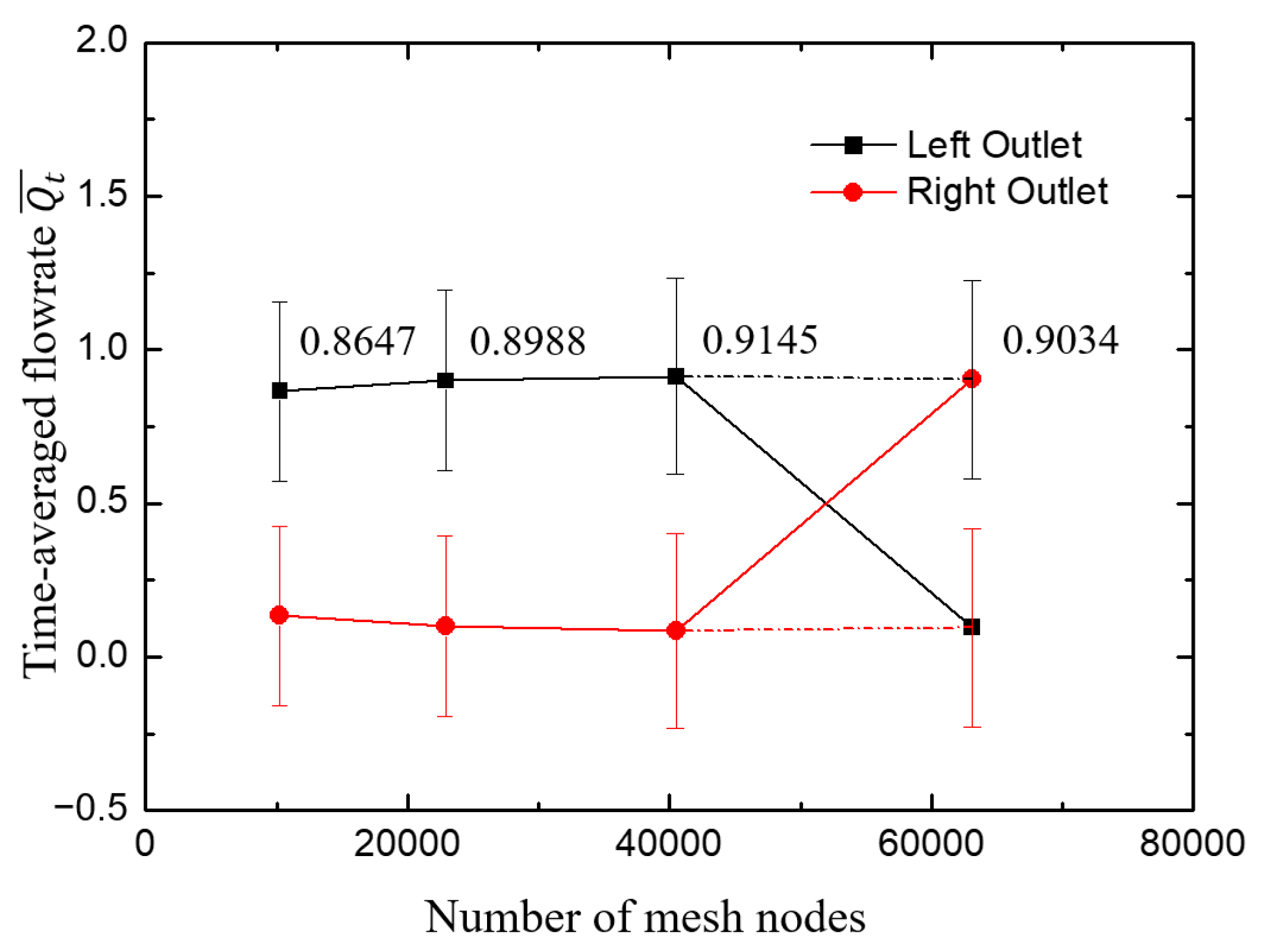
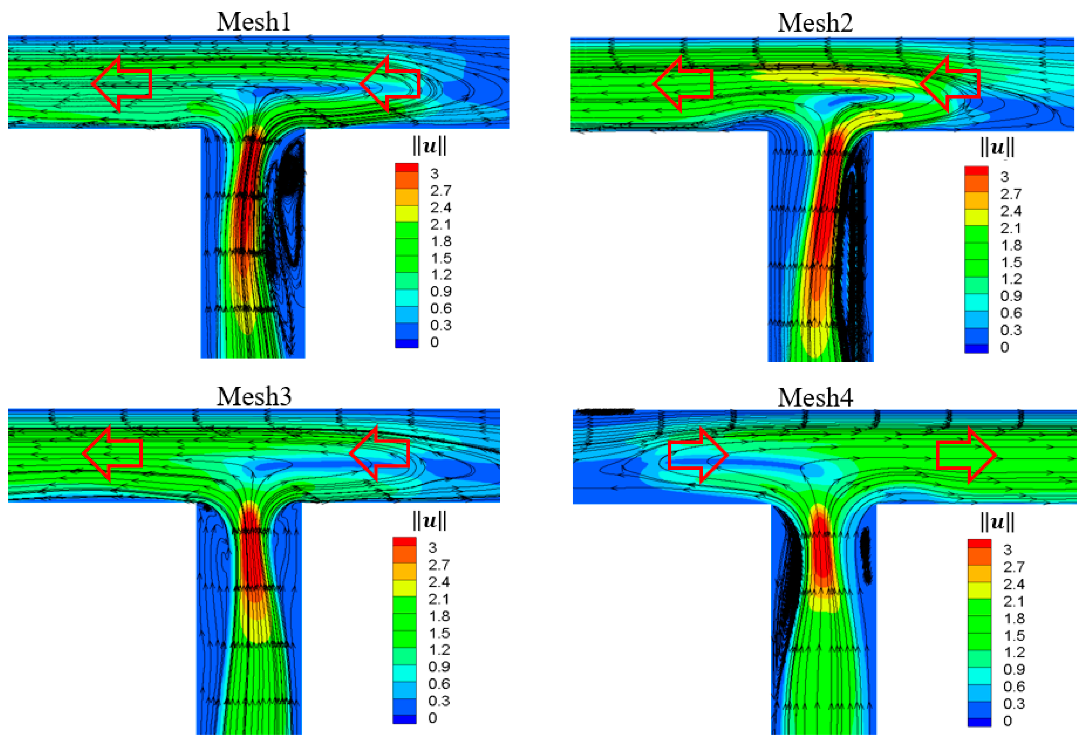
2.3. Grid Independence Validation
3. Results and Discussion
3.1. Pulsing Performance of Viscoelastic Fluid Flow in Standard T-Shaped (ST) Channel
3.2. Effect of the Weissenberg Number and Viscosity Ratio
3.3. Effect of the Channel Shape
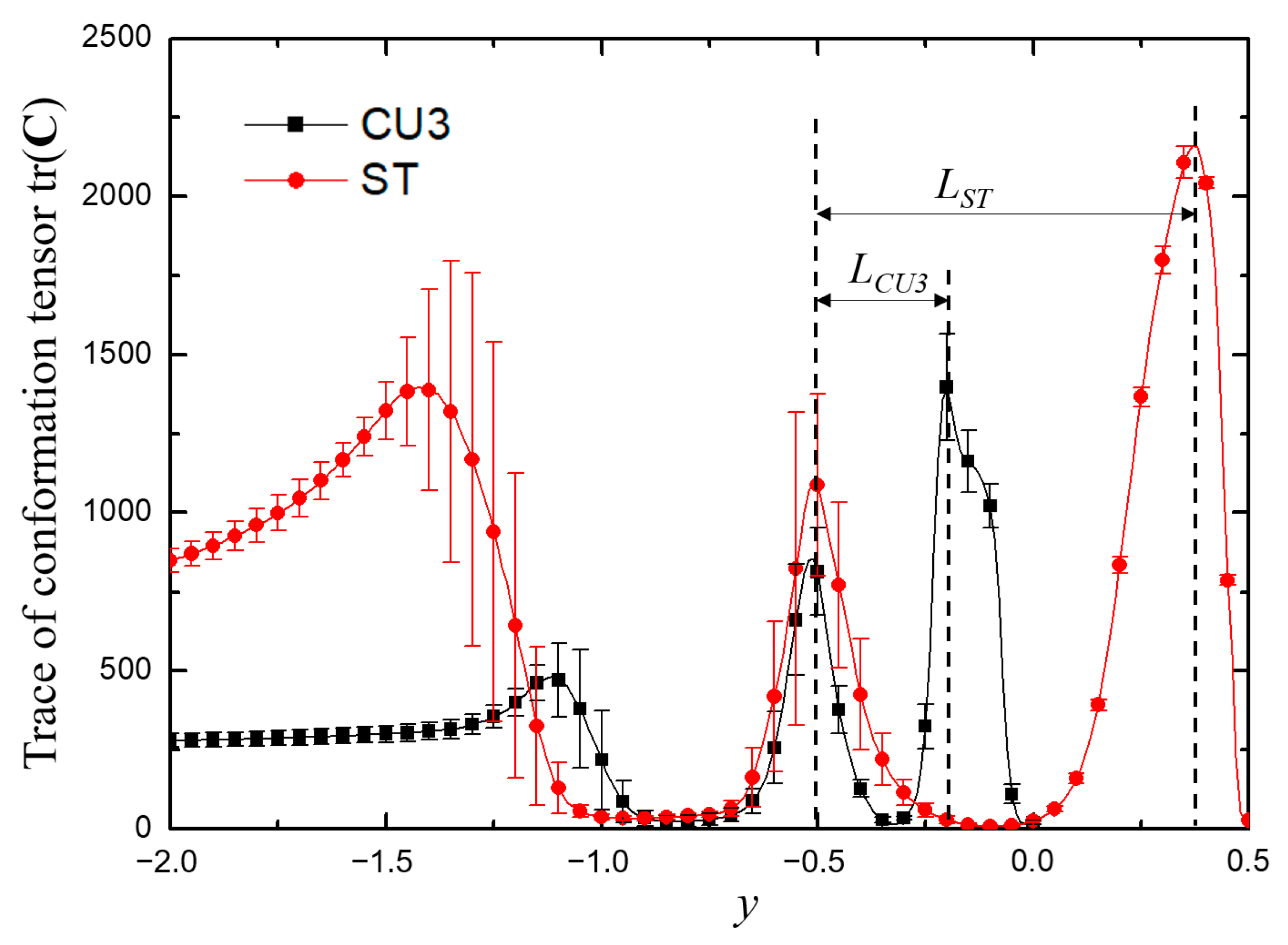
3.4. Mechanism Analysis
4. Conclusions and Outlook
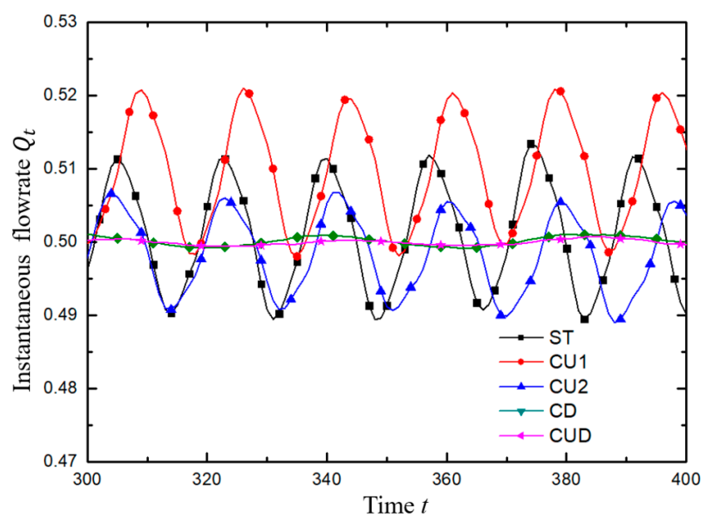
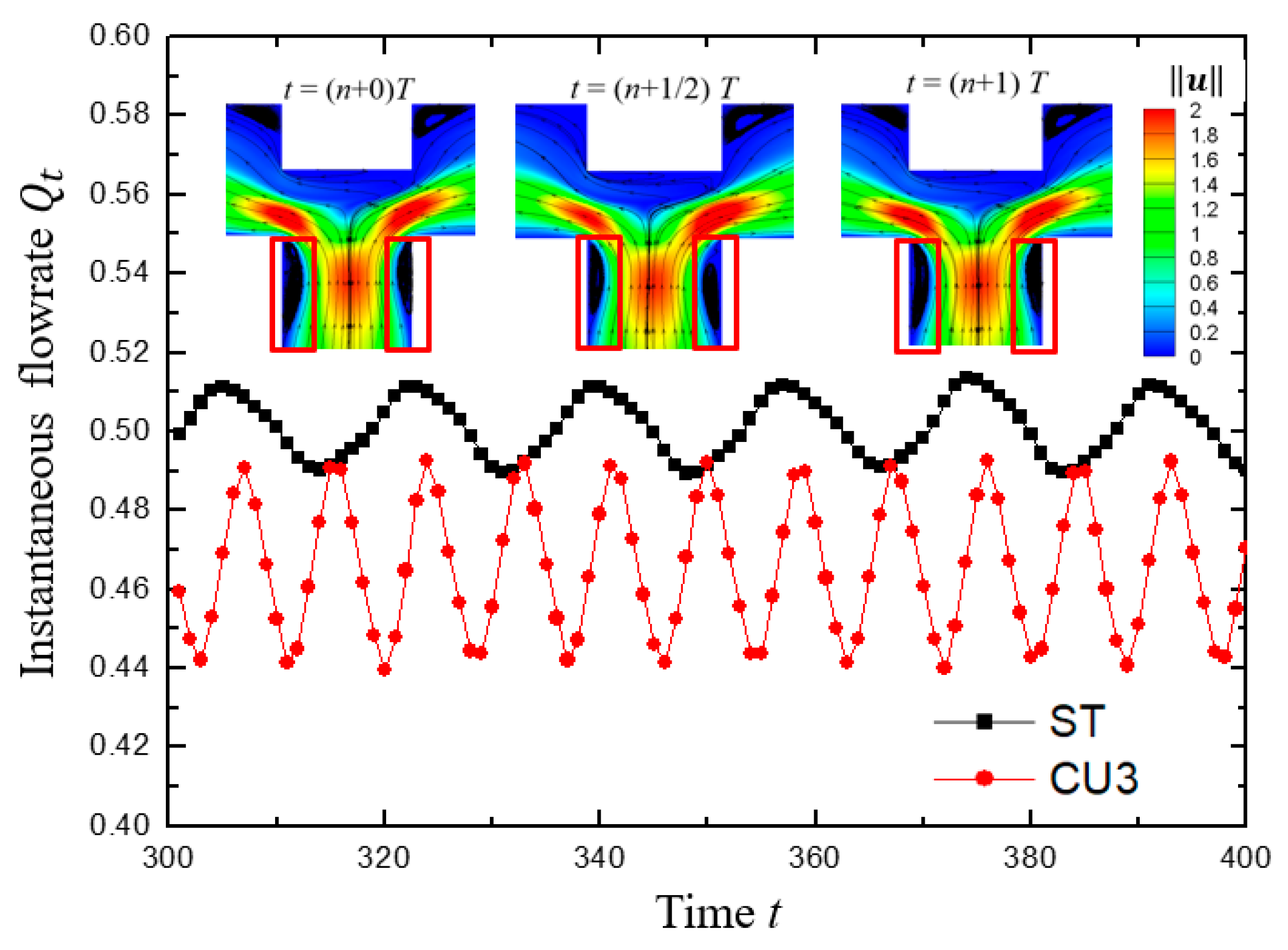
- For viscoelastic fluid with medium viscosity ratio and medium Wi the average flow rate at the outlets of standard T-shaped and its modified structures changes approximately sinusoidal-like with time;
- To generate regular periodic signals, both Wi and viscosity ratio need to be within a certain range, beyond which no oscillation or completely irregular flow will occur;
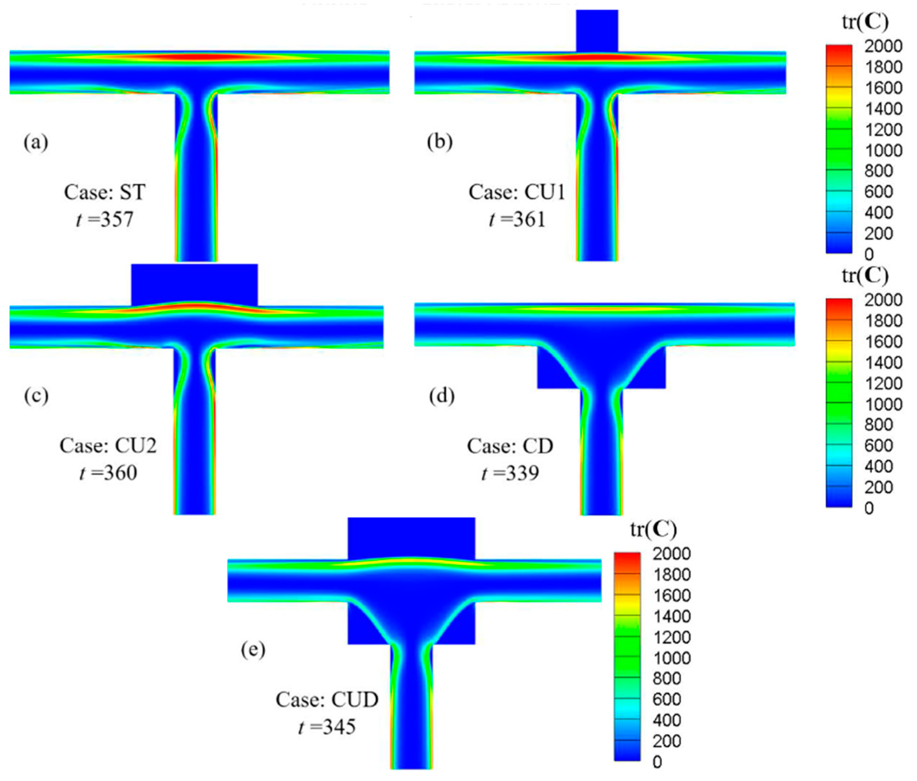
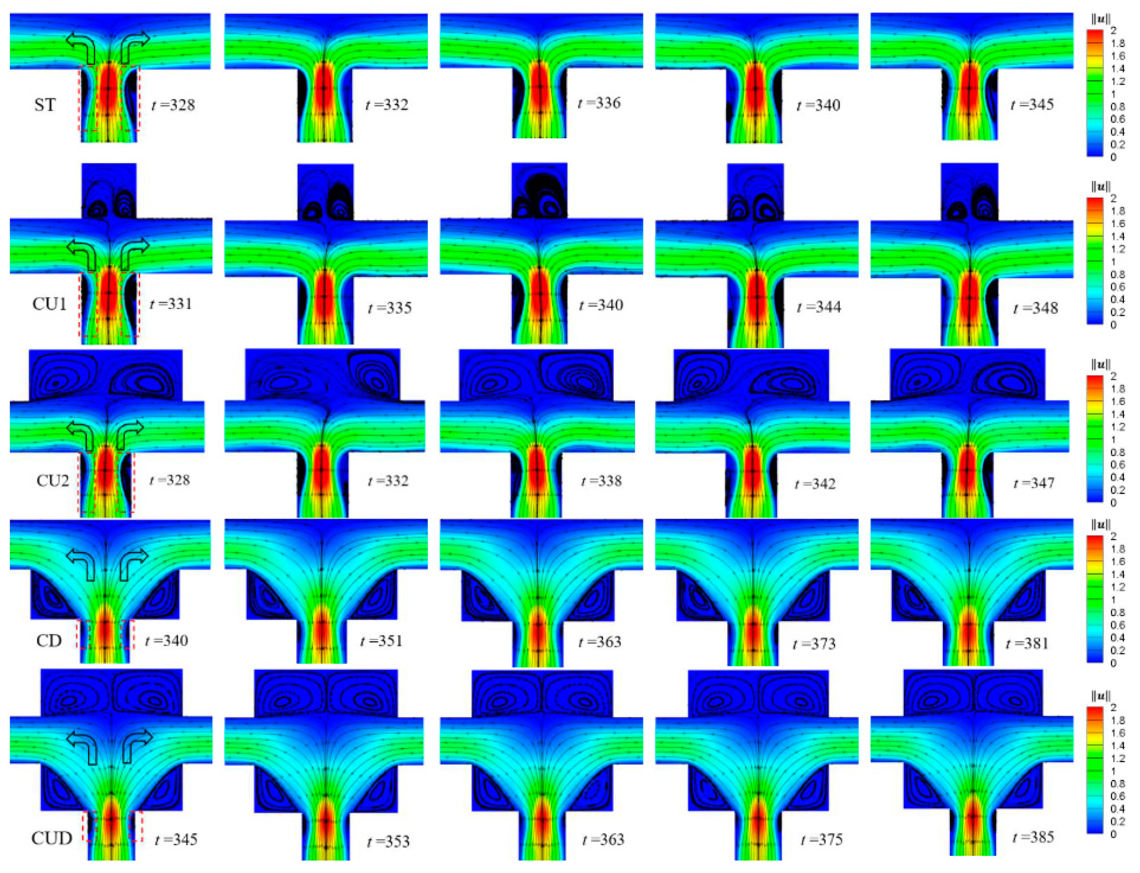
- The mechanism of the oscillation characteristics is related to the periodic fluctuation of the upstream vortex pair and the size of the elasticity-dominated area in the whole junction domain. With the presence of the dynamic evolution of the pair of vortices in the upstream near the intersection, the oscillating intensity increases as the elasticity-dominated area in the junction enlarges;
- When the T-type simple structure is considered as the potential realization of the oscillator, for now, the modified structure with a groove carved inwards on the upper wall facing the entrance branch is the most suitable for the oscillator to provide excitation for the downstream equipment.
Author Contributions
Funding
Conflicts of Interest
Nomenclature
| conformation tensor | |
| Wi | Weissenberg number |
| f | frequency |
| f0 | fundamental frequency |
| h | channel width |
| unit tensor | |
| L | A measure of the elastic effect area in the junction domain |
| pressure | |
| Qt | instantaneous flow rate |
| mean flow rate | |
| Re | Reynolds number |
| t | time |
| T | period |
| velocity vector | |
| u* | normalized streamwise velocity |
| average flow velocity in the inflow | |
| x, y | coordinates |
| Greek symbols | |
| ratio of solvent dynamic viscosity to zero-shear viscosity | |
| relaxation time of viscoelastic fluid | |
| standard deviation | |
| zero-shear fluid viscosity | |
| dynamic viscosity of the solute | |
| dynamic viscosity of the solvent | |
| density | |
| elastic stress | |
| Superscripts | |
| T | transpose operator |
| Subscripts | |
| i, j | tensor representation |
References
- Tesar, V. Oscillator micromixer. Chem. Eng. J. 2009, 155, 789–799. [Google Scholar] [CrossRef]
- Dennai, B.; Khelfaoui, R.; Benyoucef, B.; Abdenbi, A. Flow control mono and bi-stable fluidic device for micromixer-injection system. Energy Procedia 2012, 18, 571–580. [Google Scholar]
- Dennai, B.; Bentaleb, A.; Chekifi, T.; Khelfaoui, R.; Abdenbi, A. Micro fluidic oscillator: A technical solution for micro mixture. Adv. Mat. Res. 2015, 1064, 213–218. [Google Scholar] [CrossRef]
- Narumanchi, S.; Kelly, K.; Mihalic, M.; Gopalan, S.; Hester, R.; Vlahinos, A. Single-phase self-oscillating jets for enhanced heat transfer. In Proceedings of the Semitherm Conference, San Jose, CA, USA, 16–20 March 2008. [Google Scholar]
- Tesar, V. Enhancing impinging jet heat or mass transfer by fluidically generated flow pulsation. Chem. Eng. Res. Des. 2009, 87, 181–192. [Google Scholar] [CrossRef]
- Lundgreen, R.K.; Hossain, M.A.; Prenter, R.; Bons, J.P.; Gregory, J.; Ameri, A. Impingement Heat Transfer Characteristics of a Sweeping Jet. In Proceedings of the 55th AIAA Aerospace Sciences Meeting, Grapevine, TX, USA, 10 January 2017. [Google Scholar]
- Raman, G.; Cain, A.B. Innovative actuators for active flow and noise control. J. Aerosp. Eng. 2002, 216, 303–324. [Google Scholar] [CrossRef]
- Raman, G.; Raghu, S. Cavity Resonance Suppression Using Miniature Fluidic Oscillators. AIAA J. 2004, 42, 2608–2612. [Google Scholar] [CrossRef]
- Gregory, J.; Tomac, M.N. A Review of Fluidic Oscillator Development. In Proceedings of the 43rd Fluid Dynamics Conference, San Diego, CA, USA, 22 June 2013. [Google Scholar]
- Raman, G.; Packiarajan, S.; Papadopoulos, G.; Weissman, C.; Raghu, S. Jet thrust vectoring using a miniature fluidic oscillator. Aeronaut. J. 2005, 109, 129–138. [Google Scholar] [CrossRef] [Green Version]
- Khalde, C.M.; Pandit, A.V.; Sangwai, J.S.; Ranade, V.V. Flow, mixing, and heat transfer in fluidic oscillators. Can. J. Chem. Eng. 2019, 97, 542–559. [Google Scholar] [CrossRef] [Green Version]
- Dietsche, C.; Mutlu, B.R.; Edd, J.F.; Koumoutsakos, P.; Toner, M. Dynamic particle ordering in oscillatory inertial microfluidics. Microfluid. Nanofluid. 2019, 23, 83. [Google Scholar] [CrossRef]
- Mutlu, B.R.; Edd, J.F.; Toner, M. Oscillatory inertial focusing in infinite microchannels. Proc. Natl. Acad. Sci. USA 2018, 115, 7682–7687. [Google Scholar] [CrossRef] [Green Version]
- Benavides, E.M. Heat transfer enhancement by using pulsating flows. J. Appl. Phys. 2009, 105, 094907. [Google Scholar] [CrossRef]
- Wu, J.W.; Xia, H.M.; Zhang, Y.Y.; Zhao, S.F.; Zhu, P.; Wang, Z.P. An efficient micromixer combining oscillatory flow and divergent circular chambers. Microsyst. Technol. 2019, 25, 2741–2750. [Google Scholar] [CrossRef]
- Lee, G.B.; Kuo, T.Y.; Wu, W.Y. A novel micromachined flow sensor using periodic flapping motion of a planar jet impinging on a V-shaped plate. Exp. Therm. Fluid Sci. 2002, 26, 435–444. [Google Scholar] [CrossRef]
- Gregory, J.W.; Sullivan, J.P.; Raghu, S. Characterization of the microfluidic oscillator. AIAA J. 2007, 45, 568–576. [Google Scholar] [CrossRef]
- Sun, C.-L.; Sun, C.-Y. Effective mixing in a microfluidic oscillator using an impinging jet on a concave surface. Microsyst. Technol. 2011, 17, 911–922. [Google Scholar] [CrossRef]
- Zheng, M.; Mackley, M. The axial dispersion performance of an oscillatory flow meso-reactor with relevance to continuous flow operation. Chem. Eng. Sci. 2008, 63, 1788–1799. [Google Scholar] [CrossRef]
- Phan, A.N.; Harvey, A.; Lavender, J. Characterisation of fluid mixing in novel designs of mesoscale oscillatory baffled reactors operating at low flow rates (0.3–0.6 mL/min). Chem. Eng. Process. 2011, 50, 254–263. [Google Scholar] [CrossRef]
- Olayiwola, B.; Walzel, P. Effects of in-phase oscillation of retentate and filtrate in crossflow filtration at low Reynolds number. J. Membr. Sci. 2009, 345, 36–46. [Google Scholar] [CrossRef]
- Li, Z.; Dey, P.; Kim, S.-J. Microfluidic single valve oscillator for blood plasma filtration. Sens. Actuators B Chem. 2019, 296, 126692. [Google Scholar] [CrossRef]
- Lammerink, T.S.J.; Tas, N.R.; Berenschot, J.W.; Elwenspoek, M.C.; Fluitman, J.H.J. Micromachined hydraulic astable multivibrator. In Proceedings of the IEEE Micro Electro Mechanical Systems, Amsterdam, The Netherlands, 29 January–2 February 1995. [Google Scholar]
- Xie, T.L.; Xu, C. Numerical and experimental investigations of chaotic mixing behavior in an oscillating feedback micromixer. Chem. Eng. Sci. 2017, 171, 303–317. [Google Scholar] [CrossRef]
- Yang, J.T.; Chen, C.K.; Hu, I.C.; Lyu, P.C. Design of a Self-Flapping Microfluidic Oscillator and Diagnosis with Fluorescence Methods. J. Microelectromech. Syst. 2007, 16, 826–835. [Google Scholar] [CrossRef]
- Tomac, M.N.; Gregory, J. Frequency Studies and Scaling Effects of Jet Interaction in a Feedback-Free Fluidic Oscillator. In Proceedings of the 50th AIAA Aerospace Sciences Meeting including the New Horizons Forum and Aerospace Exposition, Nashville, TN, USA, 9–12 January 2012. [Google Scholar]
- Bertsch, A.; Bongarzone, A.; Duchamp, M.; Renaud, P.; Gallaire, F. Feedback-free microfluidic oscillator with impinging jets. Phys. Rev. Fluids 2020, 5, 054202. [Google Scholar] [CrossRef]
- Groisman, A.; Enzelberger, M.; Quake, S.R. Microfluidic memory and control devices. Science 2003, 300, 955–958. [Google Scholar] [CrossRef] [PubMed] [Green Version]
- Prakash, M.; Gershenfeld, N. Microfluidic bubble logic. Science 2007, 315, 832–835. [Google Scholar] [CrossRef] [Green Version]
- Stucki, J.D.; Guenat, O.T. A microfluidic bubble trap and oscillator. Lab Chip 2015, 15, 4393–4397. [Google Scholar] [CrossRef] [Green Version]
- Toepke, M.W.; Abhyankar, V.V.; Beebe, D.J. Microfluidic logic gates and timers. Lab Chip 2007, 7, 1449–1453. [Google Scholar] [CrossRef]
- Zhan, W.; Crooks, R.M. Microelectrochemical logic circuits. J. Am. Chem. Soc. 2003, 125, 9934–9935. [Google Scholar] [CrossRef] [PubMed]
- Xia, H.M.; Wang, Z.P.; Fan, W.; Wijaya, A.; Wang, W.; Wang, Z.F. Converting steady laminar flow to oscillatory flow through a hydroelasticity approach at microscales. Lab Chip 2012, 12, 60–64. [Google Scholar] [CrossRef]
- Xia, H.M.; Wu, J.; Wang, Z. The negative-differential-resistance (NDR) mechanism of a hydroelastic microfluidic oscillator. J. Micromech. Microeng. 2017, 27, 075001. [Google Scholar] [CrossRef]
- Kim, S.J.; Yokokawa, R.; Lesher-Perez, S.C.; Takayama, S. Multiple independent autonomous hydraulic oscillators driven by a common gravity head. Nat. Commun. 2015, 6, 7301. [Google Scholar] [CrossRef] [Green Version]
- Kim, S.-J.; Yokokawa, R.; Lesher-Perez, S.C.; Takayama, S. Constant Flow-Driven Microfluidic Oscillator for Different Duty Cycles. Anal. Chem. 2011, 84, 1152–1156. [Google Scholar] [CrossRef] [Green Version]
- McKinley, G.H.; Pakdel, P.; Oztekin, A. Rheological and geometric scaling of purely elastic flow instabilities. J. Non-Newton. Fluid. 1996, 67, 19–47. [Google Scholar] [CrossRef]
- Pakdel, P.; McKinley, G.H. Elastic instability and curved streamlines. Phys. Rev. Lett. 1996, 77, 2459–2462. [Google Scholar] [CrossRef] [PubMed]
- Groisman, A.; Steinberg, V. Elastic turbulence in a polymer solution flow. Nature 2000, 405, 53–55. [Google Scholar] [CrossRef] [PubMed] [Green Version]
- Yuan, C.; Zhang, H.N.; Li, Y.K.; Li, X.B.; Wu, J.; Li, F.C. Nonlinear effects of viscoelastic fluid flows and applications in microfluidics: A review. Proc. Inst. Mech. Eng. Part C J. Eng. Mech. Eng. Sci. 2020, 234, 4390–4414. [Google Scholar] [CrossRef]
- Asghari, M.; Cao, X.; Mateescu, B.; van Leeuwen, D.; Aslan, M.K.; Stavrakis, S.; deMello, A.J. Oscillatory Viscoelastic Microfluidics for Efficient Focusing and Separation of Nanoscale Species. ACS Nano 2020, 14, 422–433. [Google Scholar] [CrossRef] [PubMed]
- Sun, C.-l.; Lin, Y.J.; Rau, C.-I.; Chiu, S.-Y. Flow characterization and mixing performance of weakly-shear-thinning fluid flows in a microfluidic oscillator. J. Non-Newton. Fluid 2017, 239, 1–12. [Google Scholar] [CrossRef]
- Matos, H.M.; Oliveira, P.J. Steady flows of constant-viscosity viscoelastic fluids in a planar T-junction. J. Non-Newton. Fluid 2014, 213, 15–26. [Google Scholar] [CrossRef]
- Li, X.-B.; Li, F.-C.; Kinoshita, H.; Oishi, M.; Oshima, M. Dynamics of viscoelastic fluid droplet under very low interfacial tension in a serpentine T-junction microchannel. Microfluid. Nanofluid. 2014, 18, 1007–1021. [Google Scholar] [CrossRef]
- Colin, M.; Colin, T.; Dambrine, J. Numerical simulations of wormlike micelles flows in micro-fluidic T-shaped junctions. Math. Comput. Simulat. 2016, 127, 28–55. [Google Scholar] [CrossRef]
- Soulages, J.; Oliveira, M.S.N.; Sousa, P.C.; Alves, M.A.; McKinley, G.H. Investigating the stability of viscoelastic stagnation flows in T-shaped microchannels. J. Non-Newton. Fluid 2009, 163, 9–24. [Google Scholar] [CrossRef] [Green Version]
- Varshney, A.; Afik, E.; Kaplan, Y.; Steinberg, V. Oscillatory elastic instabilities in an extensional viscoelastic flow. Soft Matter 2016, 12, 2186–2191. [Google Scholar] [CrossRef] [Green Version]
- Poole, R.J.; Alfateh, M.; Gauntlett, A.P. Bifurcation in a T-channel junction: Effects of aspect ratio and shear-thinning. Chem. Eng. Sci. 2013, 104, 839–848. [Google Scholar] [CrossRef]
- Poole, R.J.; Haward, S.J.; Alves, M.A. Symmetry-breaking bifurcations in T-channel flows: Effects of fluid viscoelasticity. Procedia Eng. 2014, 79, 28–34. [Google Scholar] [CrossRef] [Green Version]
- Keslerova, R.; Trdlicka, D. Numerical solution of viscous and viscoelastic fluids flow through the branching channel by finite volume scheme. J. Phys. Conf. Ser. 2015, 633, 012128. [Google Scholar] [CrossRef] [Green Version]
- Miranda, A.I.P.; Oliveira, P.J.; Pinho, F.T. Steady and unsteady laminar flows of Newtonian and generalized Newtonian fluids in a planar T-junction. Int. J. Numer. Methods Fluids 2008, 57, 295–328. [Google Scholar] [CrossRef]
- Mosadegh, B.; Kuo, C.H.; Tung, Y.C.; Torisawa, Y.S.; Bersano-Begey, T.; Tavana, H.; Takayama, S. Integrated elastomeric components for autonomous regulation of sequential and oscillatory flow switching in microfluidic devices. Nat. Phys. 2010, 6, 433–437. [Google Scholar] [CrossRef] [PubMed] [Green Version]
- Bird, R.B.; Curtiss, C.F.; Armstrong, R.C.; Hassager, O. Dynamics of Polymeric Liquids: Kinetic Theory; John Wiley and Sons Inc.: New York, NY, USA, 1987. [Google Scholar]
- van Buel, R.; Stark, H. Active open-loop control of elastic turbulence. Sci. Rep. UK 2020, 10, 15704. [Google Scholar] [CrossRef] [PubMed]
- Canossi, D.O.; Mompean, G.; Berti, S. Elastic turbulence in two-dimensional cross-slot viscoelastic flows. EPL 2020, 129, 24002. [Google Scholar] [CrossRef]
- Yuan, C.; Zhang, H.N.; Chen, L.X.; Zhao, J.L.; Li, X.B.; Li, F.C. Numerical Study on the Characteristics of Boger Type Viscoelastic Fluid Flow in a Micro Cross-Slot under Sinusoidal Stimulation. Entropy 2020, 22, 64. [Google Scholar] [CrossRef] [PubMed] [Green Version]
- Sousa, P.C.; Pinho, F.T.; Oliveira, M.S.N.; Alves, M.A. Purely elastic flow instabilities in microscale cross-slot devices. Soft Matter 2015, 11, 8856–8862. [Google Scholar] [CrossRef] [Green Version]
- Davoodi, M.; Domingues, A.; Poole, R. Control of a purely elastic symmetry-breaking flow instability in cross-slot geometries. J. Fluid Mech. 2019, 881, 1123–1157. [Google Scholar] [CrossRef] [Green Version]
- Zhang, H.N.; Li, D.Y.; Li, X.B.; Cai, W.H.; Li, F.C. Numerical simulation of heat transfer process of viscoelastic fluid flow at high Weissenberg number by log-conformation reformulation. J. Fluid. Eng. T. ASME 2017, 139, 091402. [Google Scholar] [CrossRef]
- Yeh, L.H.; Hsu, J.P. Electrophoresis of a finite rod along the axis of a long cylindrical microchannel filled with Carreau fluids. Microfluid. Nanofluid. 2009, 7, 383–392. [Google Scholar] [CrossRef]


| Category | Characteristic | Channel Shape | Channel Width (μm) | Channel Depth (μm) | Fluid/Model | Re | f (Hz) | Reference |
|---|---|---|---|---|---|---|---|---|
| Electronic–fluidic analogy based | Fluidic circuit is analogous to electronic astable multivibrator | 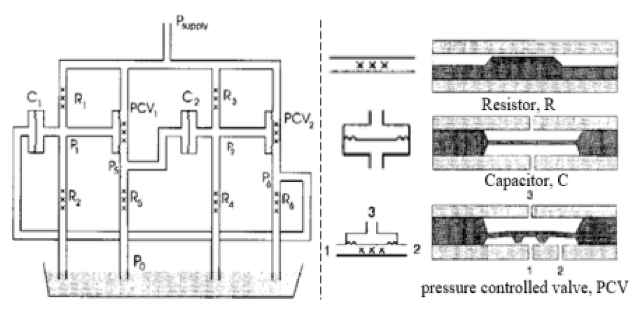 | ~30 | n/a | Water; CAMAS program package | n/a | 0.18 | [23] a |
| Coanda effect | Symmetric feedback channel |  | 200 | n/a | DI water; DNS | 16.7~100 | ~180 | [24] a |
| Asymmetric feedback channel |  | 16 | 263 | DI water; DNS | 1~100 | ~1 | [25] a | |
| Elastic diaphragm | The hydroelasticity realized by a four-layer substrate with a diaphragm embedded in between introduces nonlinearity | 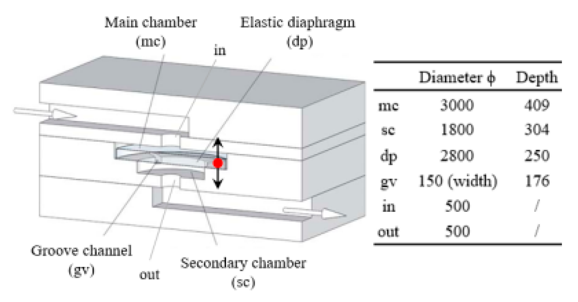 | 2800 | n/a | 50% glycerol–50% water solution | 10~100 | ~210 | [33] b |
| The combination of switch-valves and check-valves that both contain a diaphragm as a core element | 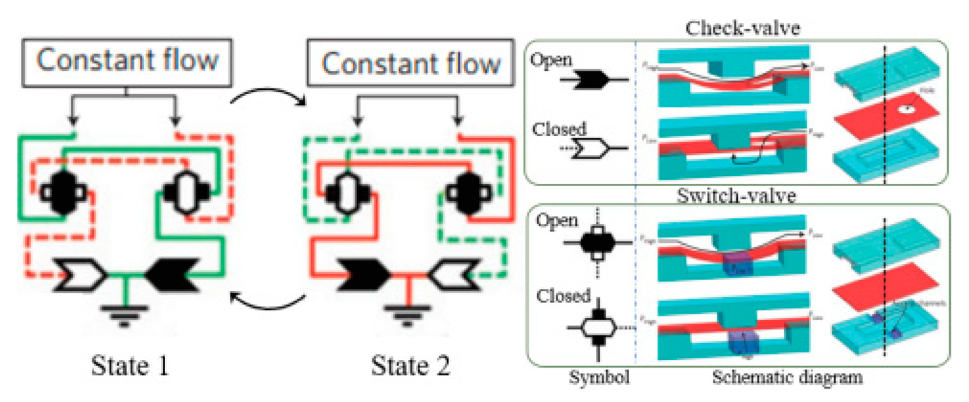 | n/a | 100 | Water LabVIEW | n/a | ~1 | [52] a | |
| Impinging-jet-based | A planar jet impinges on a V-shaped plate downstream |  | 1440, 2790 | 48 | water | 0.2~5.4 | ~0.3 | [16] b |
| Secondary flow induces Gortler instability | 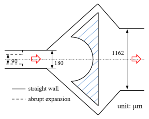 | 180 | 218.1 | distilled water | 50~450 | 0.1~0.6 | [18] b | |
| Interaction of two jets with intersecting angles | 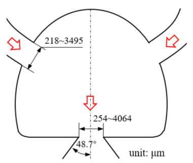 | 254~4064 | 152.4~2423 | air, argon, hydrogen, pure water and sodium iodide solution; SST model | ~104 | ~3 × 10⁴ (hydrogen) | [26] a | |
| Interaction between two opposing jets | 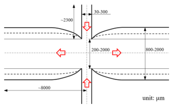 | 50~300 | 150~525 | DI water; DNS | 15~630 | 1230 | [27] a |
| Category | Exp/Num a | Channel Shape | Width h (μm) | Fluid/Model | Wi | Re | Reference | |
|---|---|---|---|---|---|---|---|---|
| Two streams collide head-on | Exp |  | 50 | 0.075 wt.% PEO (MW: 2 × 10⁶) | 29.33 | 0.5 | 0.065 | [46] |
| glycerol/water mixture (60/40 wt.%) | n/a | n/a | ||||||
| 2D | n/a | sPTT | 4.4 | 0.5 | ~0 | |||
| Exp |  | 3000 | 80 ppm PAAm (MW: 18 × 106) | ~1200 | ~0.77 | 0.1~3 | [47] | |
| Two streams leave in perpendicular | 2D |  | n/a | FENE-CR and FENE-MCR | 3 | 0.3–0.9 | 102 | [43] |
| 3D |  | 3100 | Oldroyd-B | 1.2 b | 0.9 | 50 | [50] | |
| 2D | n/a | Carreau–Yasuda | 50~1000 | n/a | n/a | [51] | ||
| Two streams collide in perpendicular | Exp | 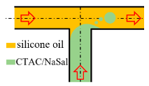 | 100 | 200, 600 and 1000 ppm CTAC with NaSal | 1.54~42.22 | n/a | n/a | [44] |
| Two streams leave in opposite directions | 3D | 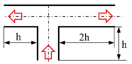 | 1000 | modified Giesekus | n/a | n/a | ~0 | [45] |
| Case | Channel Geometry a | Channel Shape | Case Illustration b | β | Wi | Re |
|---|---|---|---|---|---|---|
| Standard T (abbreviated as “ST”) | n/a |  | ST-N | 1 | 0 | 0.01 |
| ST-betaXX-WiXX | 0.1, 0.5, 0.9 | 1, 5, 10 | ||||
| Cavity_Up1 (abbreviated as “CU1”) | ② | 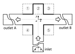 | CU1-N | 1 | 0 | |
| CU1-betaXX-WiXX | 0.1, 0.5, 0.9 | 1, 5, 10 | ||||
| Cavity_Up2 (abbreviated as “CU2”) | ①②③ | 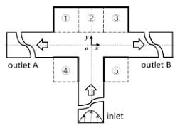 | CU2-N | 1 | 0 | |
| CU2-betaXX- WiXX | 0.1, 0.5, 0.9 | 1, 5, 10 | ||||
| Cavity_Down (abbreviated as “CD”) | ④⑤ | 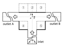 | CD-N | 1 | 0 | |
| CD-betaXX- WiXX | 0.1, 0.5, 0.9 | 1, 5, 10 | ||||
| Cavity_Up_Down (abbreviated as “CUD”) | ①②③④⑤ | 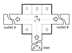 | CUD-N | 1 | 0 | |
| CUD-betaXX-WiXX | 0.1, 0.5, 0.9 | 1, 5, 10 |
| Item | NDx | NDy | NDbranch | and | NC | ND |
|---|---|---|---|---|---|---|
| Mesh1 | 51 | 51 | 51 | 0.020 | 10,508 | 10,251 |
| Mesh2 | 76 | 76 | 76 | 0.013 | 23,258 | 22,876 |
| Mesh3 | 101 | 101 | 101 | 0.010 | 41,008 | 40,501 |
| Mesh4 | 126 | 126 | 126 | 0.008 | 63,758 | 63,126 |
| ST | CU1 | CU2 | CD | CUD | |
|---|---|---|---|---|---|
| 0.5015 | 0.5077 | 0.4935 | 0.5000 | 0.4999 | |
| 0.0075 | 0.0076 | 0.0066 | 0.0006 | 0.0005 |
Publisher’s Note: MDPI stays neutral with regard to jurisdictional claims in published maps and institutional affiliations. |
© 2021 by the authors. Licensee MDPI, Basel, Switzerland. This article is an open access article distributed under the terms and conditions of the Creative Commons Attribution (CC BY) license (https://creativecommons.org/licenses/by/4.0/).
Share and Cite
Yuan, C.; Zhang, H.; Li, X.; Oishi, M.; Oshima, M.; Yao, Q.; Li, F. Numerical Investigation of T-Shaped Microfluidic Oscillator with Viscoelastic Fluid. Micromachines 2021, 12, 477. https://doi.org/10.3390/mi12050477
Yuan C, Zhang H, Li X, Oishi M, Oshima M, Yao Q, Li F. Numerical Investigation of T-Shaped Microfluidic Oscillator with Viscoelastic Fluid. Micromachines. 2021; 12(5):477. https://doi.org/10.3390/mi12050477
Chicago/Turabian StyleYuan, Chao, Hongna Zhang, Xiaobin Li, Masamichi Oishi, Marie Oshima, Qinghe Yao, and Fengchen Li. 2021. "Numerical Investigation of T-Shaped Microfluidic Oscillator with Viscoelastic Fluid" Micromachines 12, no. 5: 477. https://doi.org/10.3390/mi12050477
APA StyleYuan, C., Zhang, H., Li, X., Oishi, M., Oshima, M., Yao, Q., & Li, F. (2021). Numerical Investigation of T-Shaped Microfluidic Oscillator with Viscoelastic Fluid. Micromachines, 12(5), 477. https://doi.org/10.3390/mi12050477