


Interval Type-3 Fuzzy Adaptation of the Bee Colony Optimization Algorithm for Optimal Fuzzy Control of an Autonomous Mobile Robot


Abstract
:1. Introduction
2. Fuzzy Sets
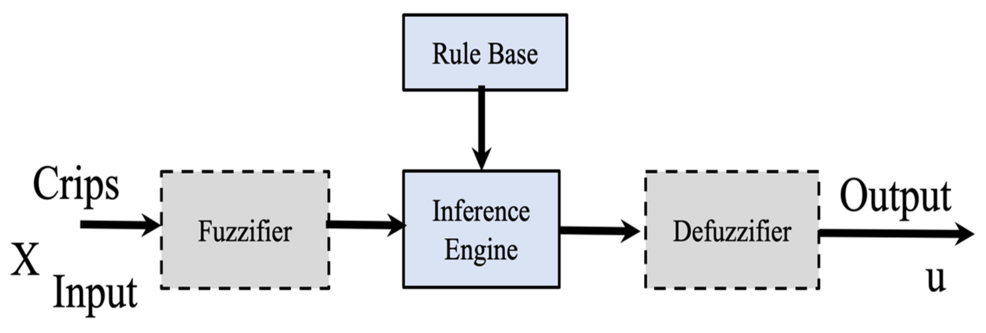
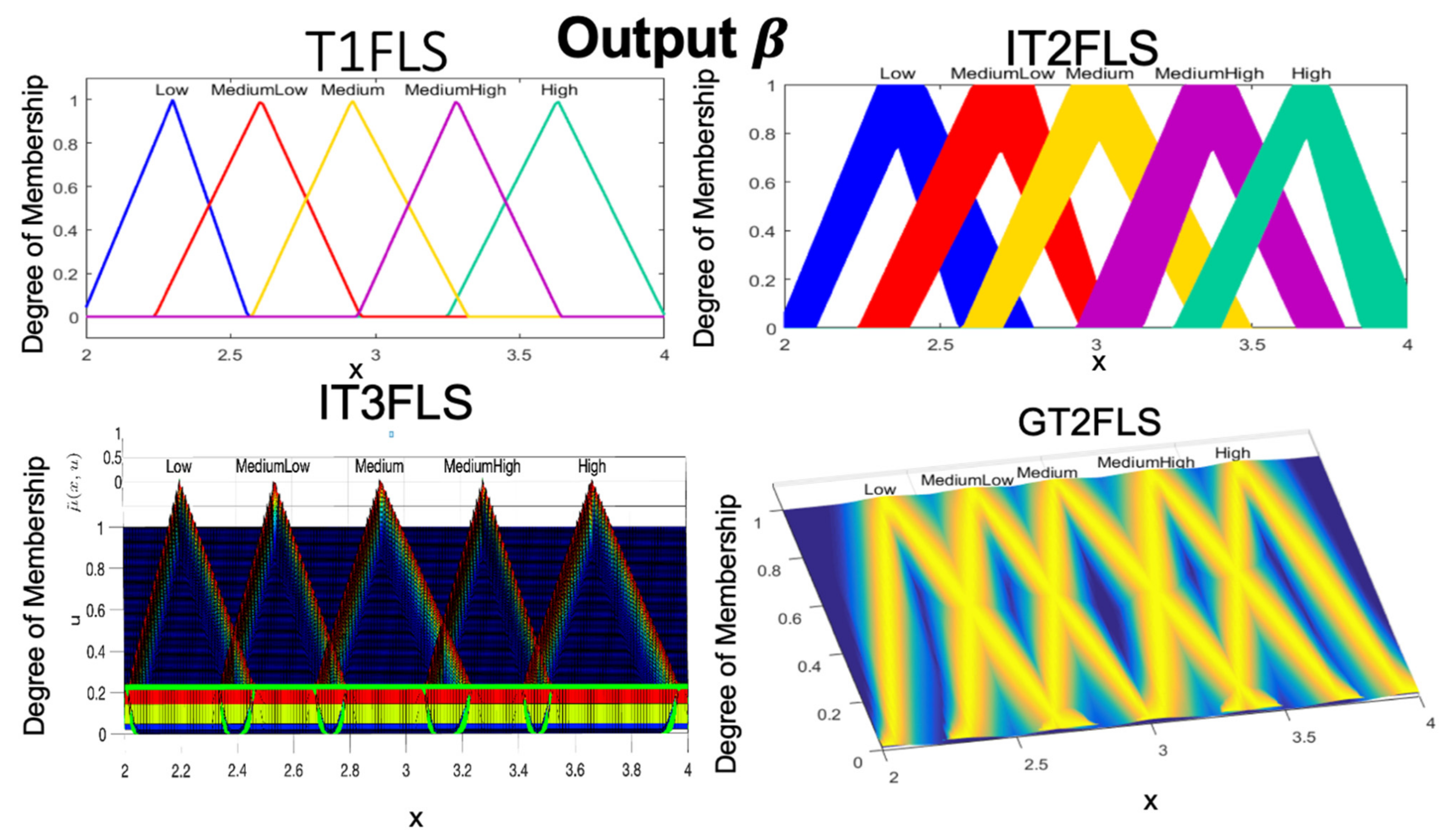
2.1. Type-1 Fuzzy Logic System
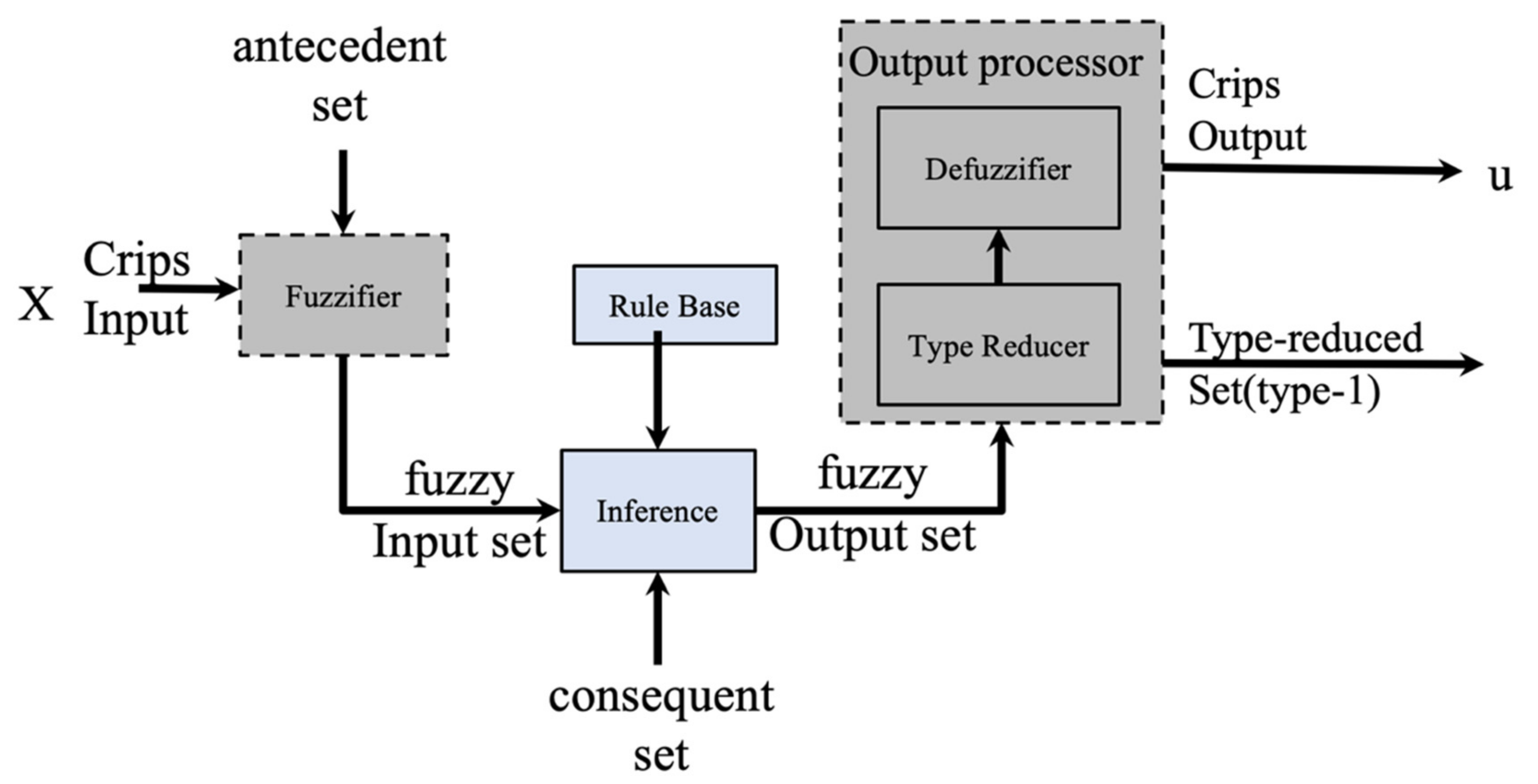
2.2. Interval Type–2 System
2.3. Generalized Type–2 System
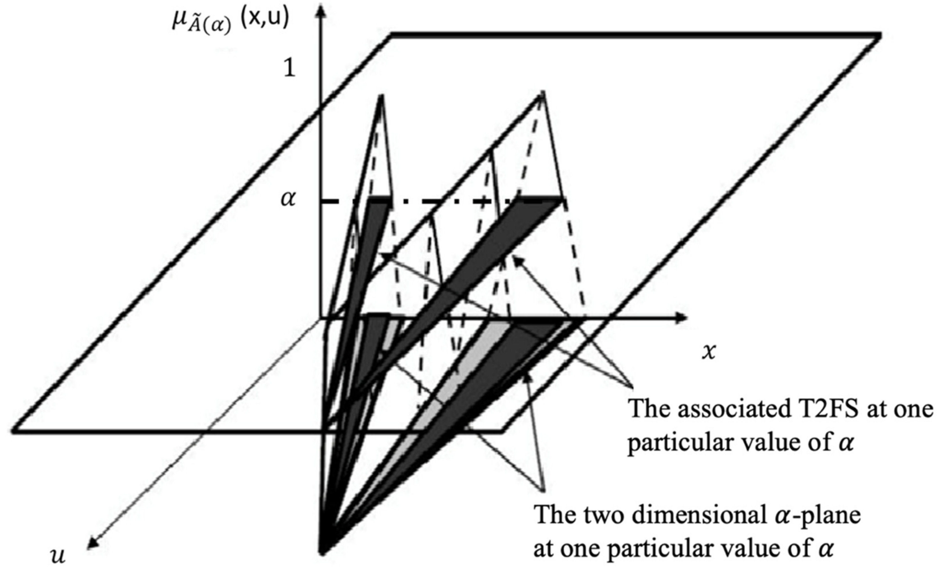
𝛼-Planes Representation
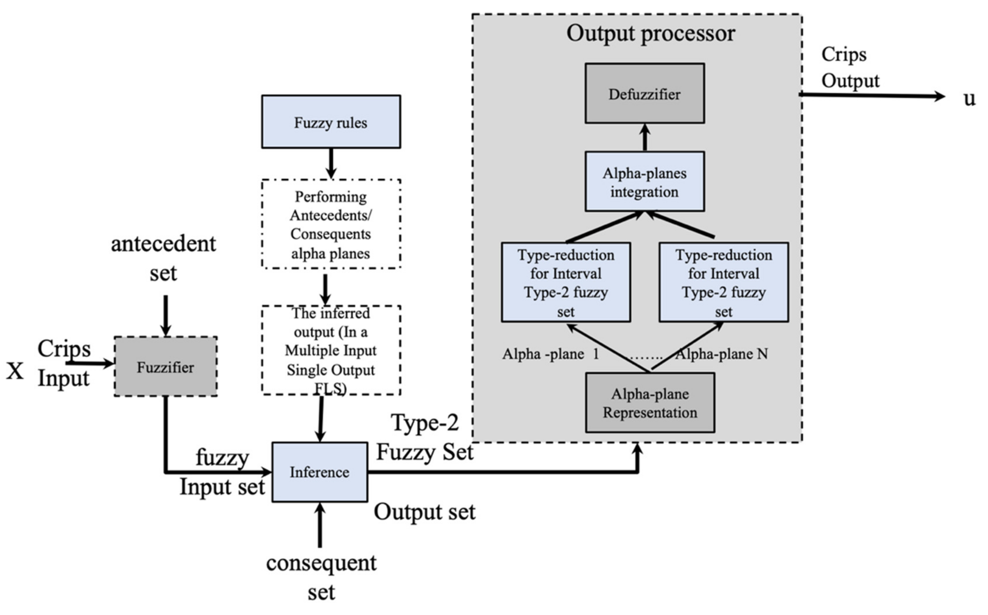
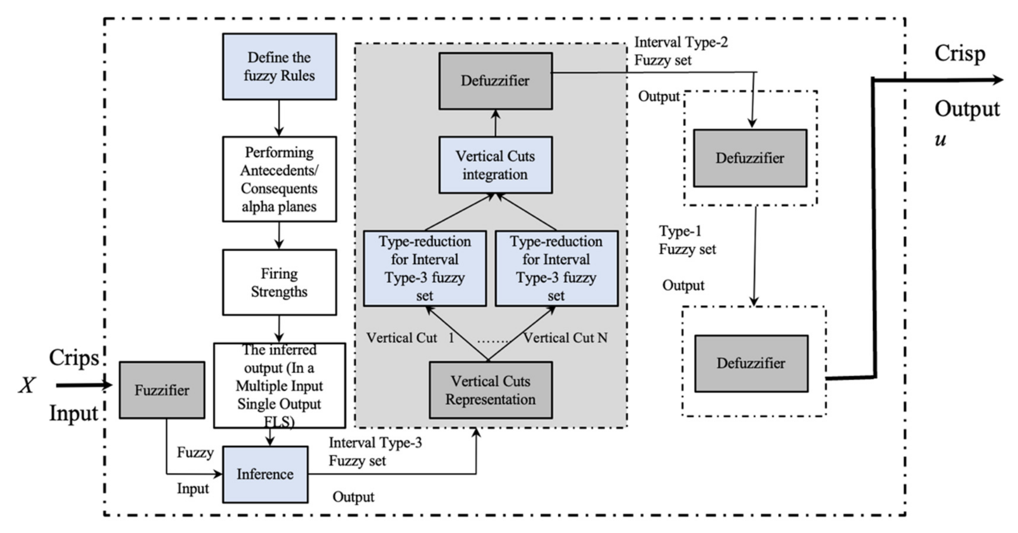
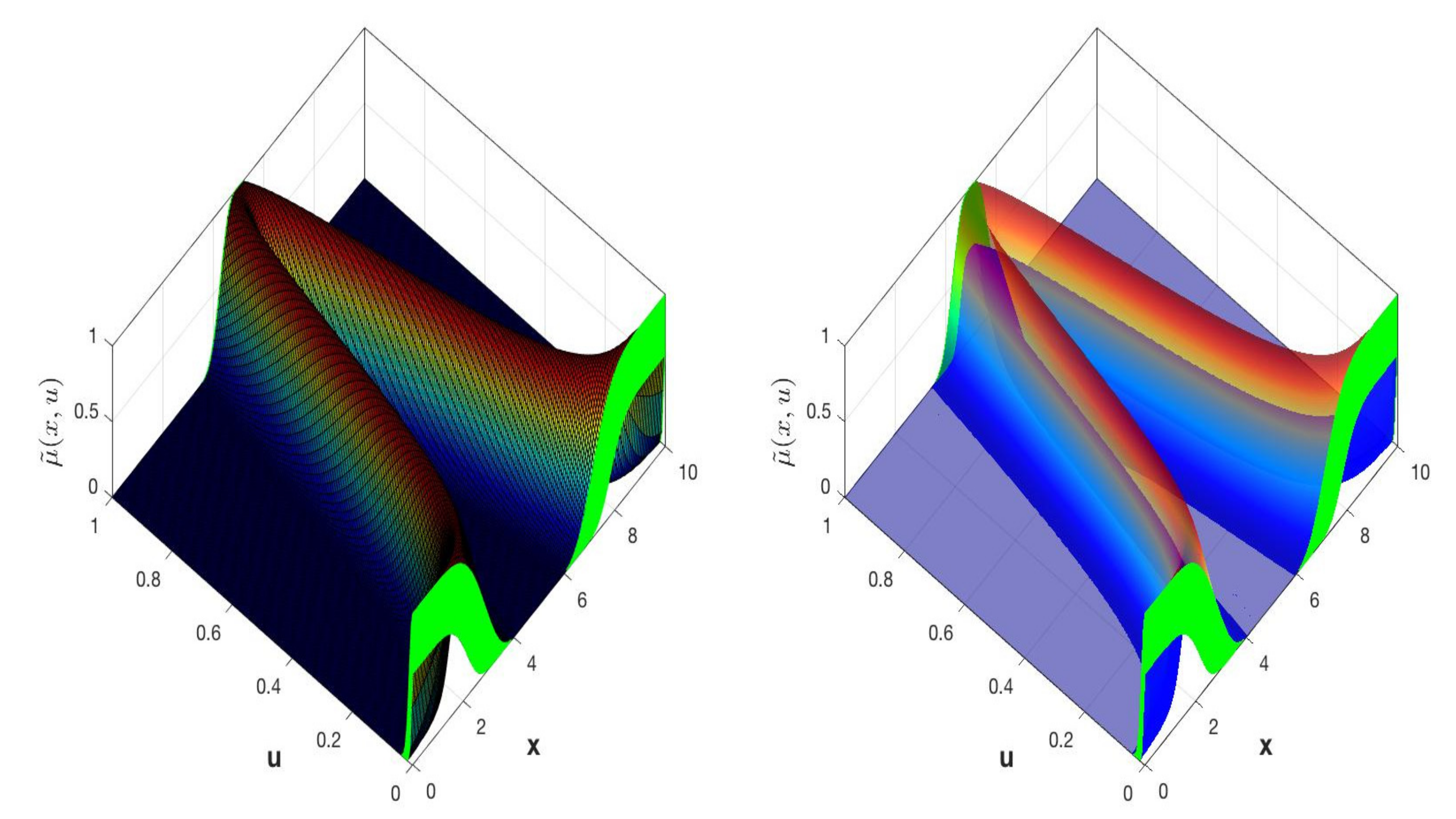
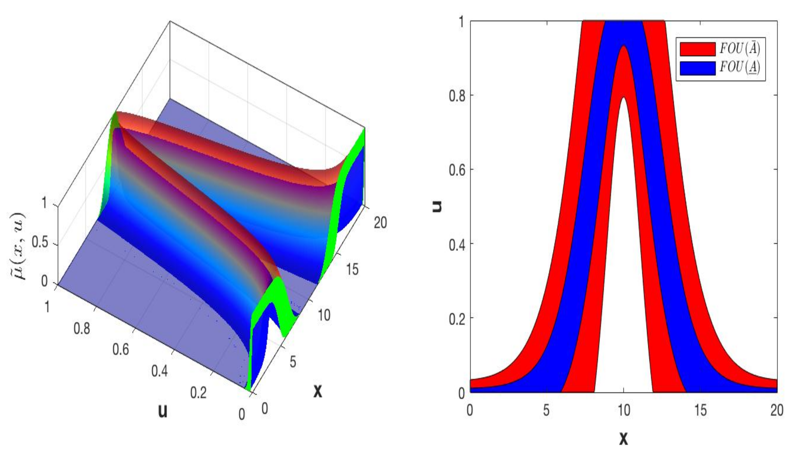
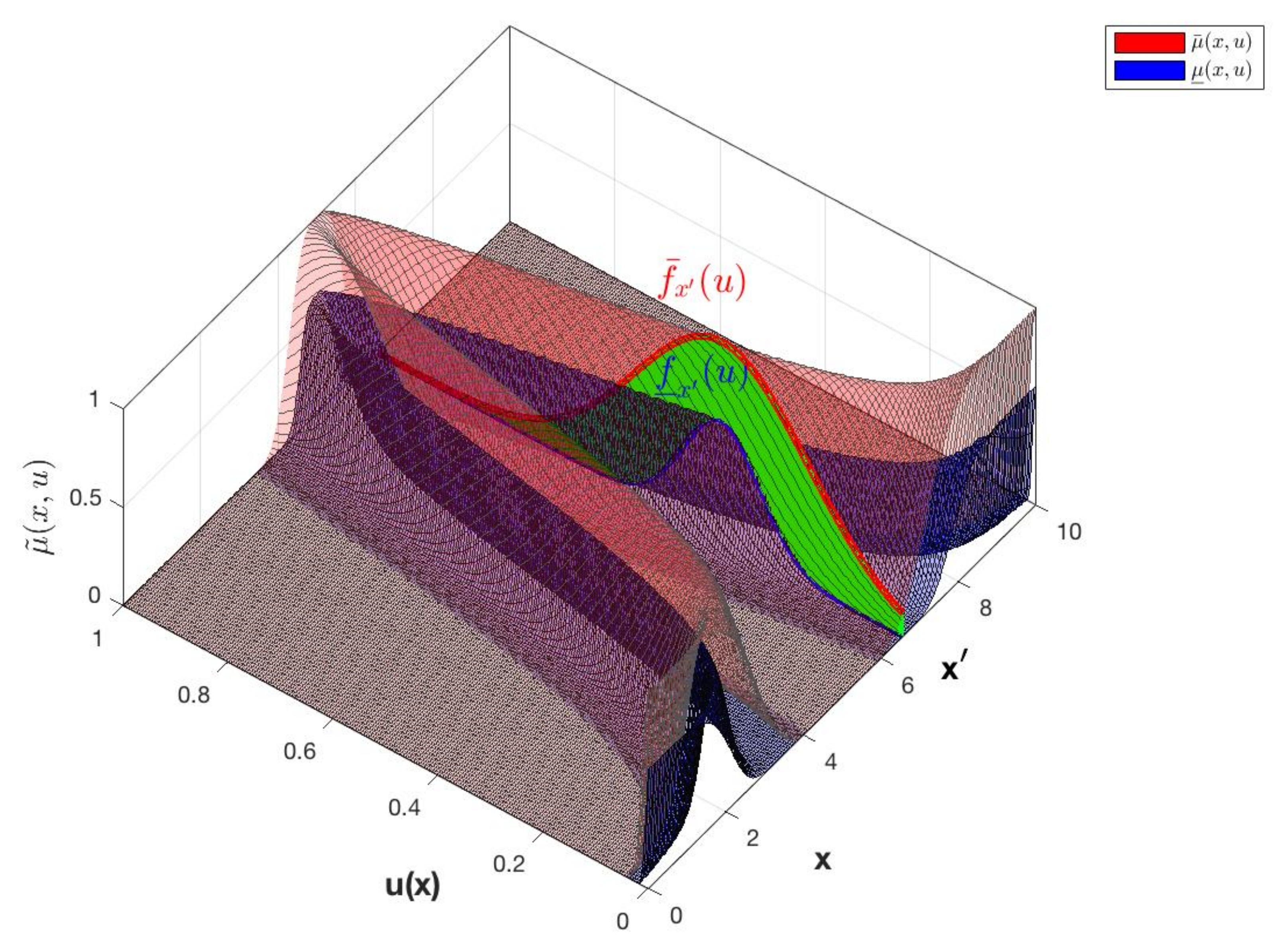
2.4. Interval Type–3 System
2.4.1. Fuzzification
2.4.2. Inference
2.4.3. Vertical Slice Representation
2.4.4. Type Reductor
2.4.5. Defuzzification
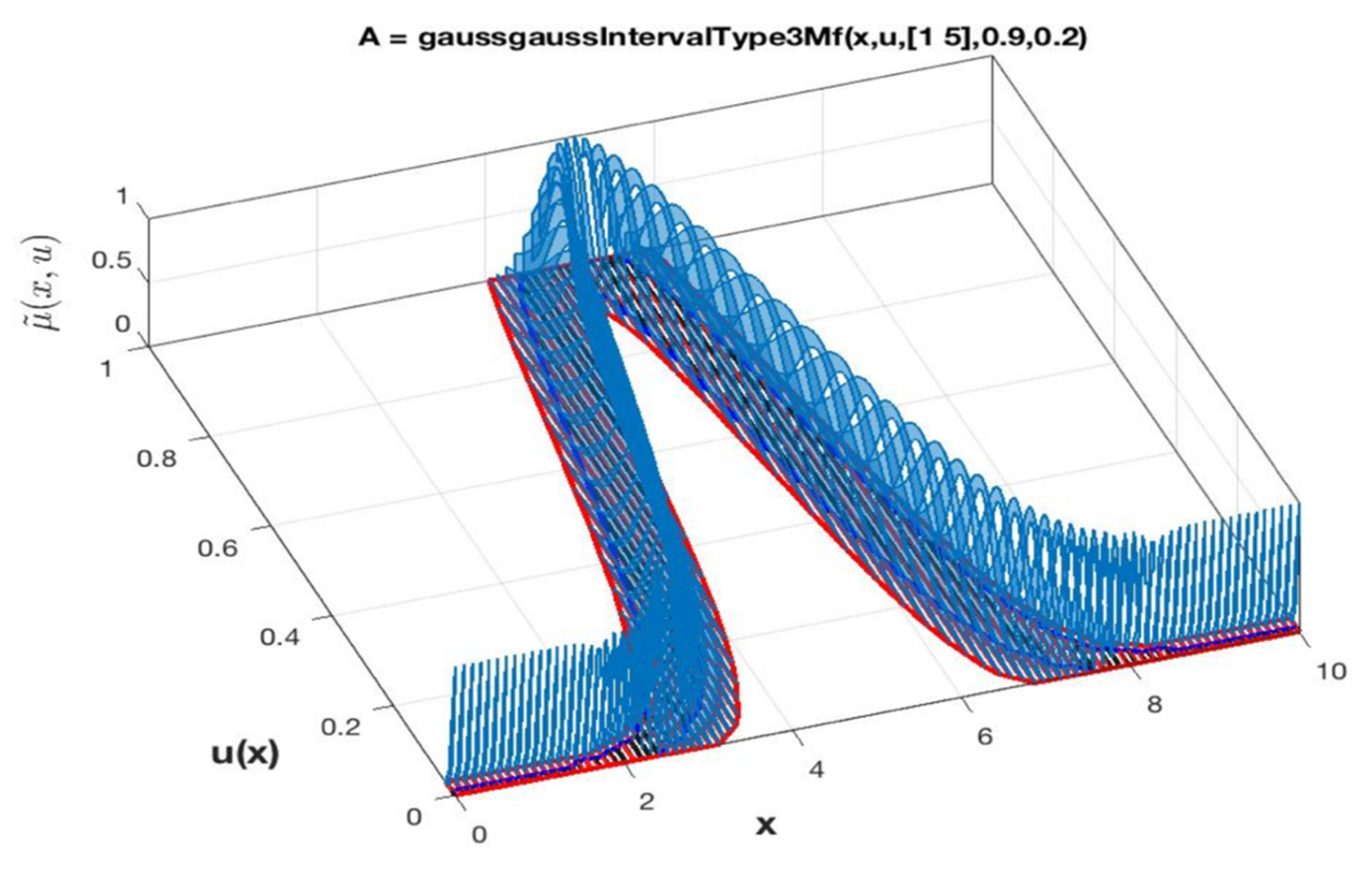
2.5. Mathematical Representation for ScaleTriScaleGaussIT3MF
3. Study Case
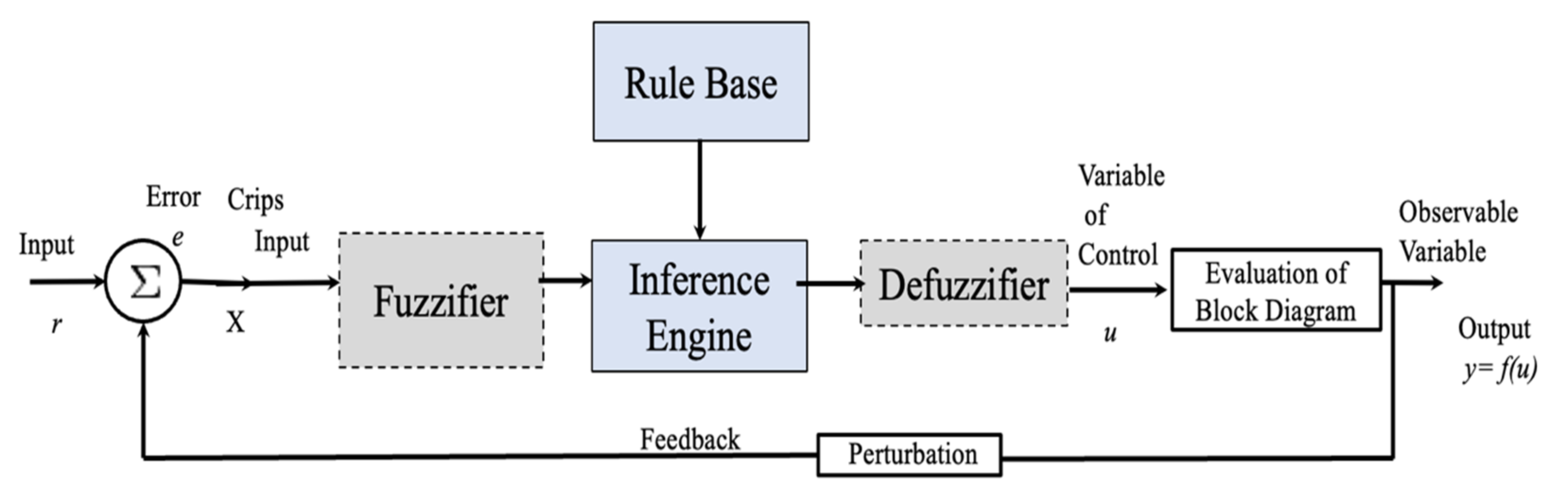
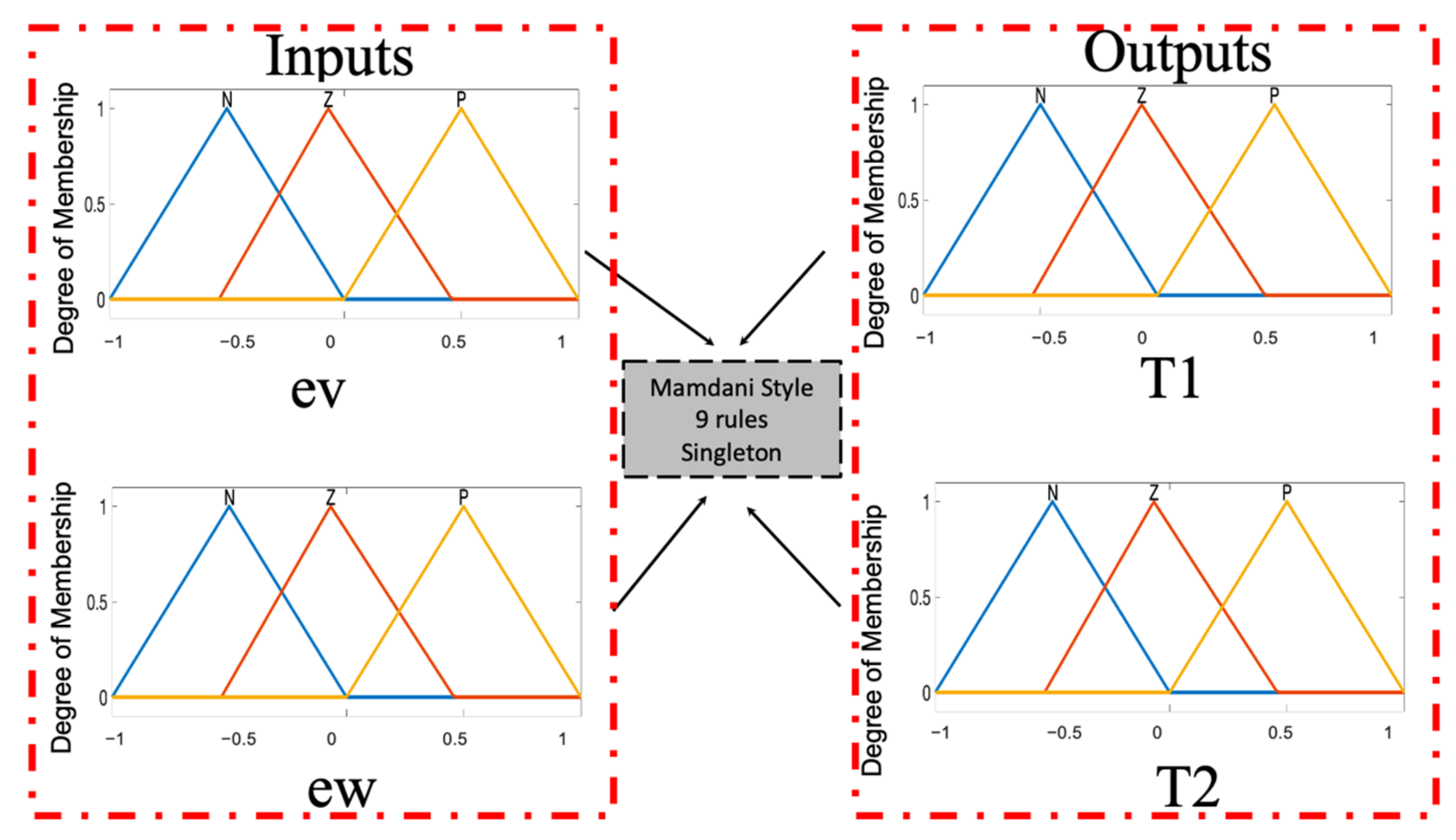
3.1. Fuzzy Controller
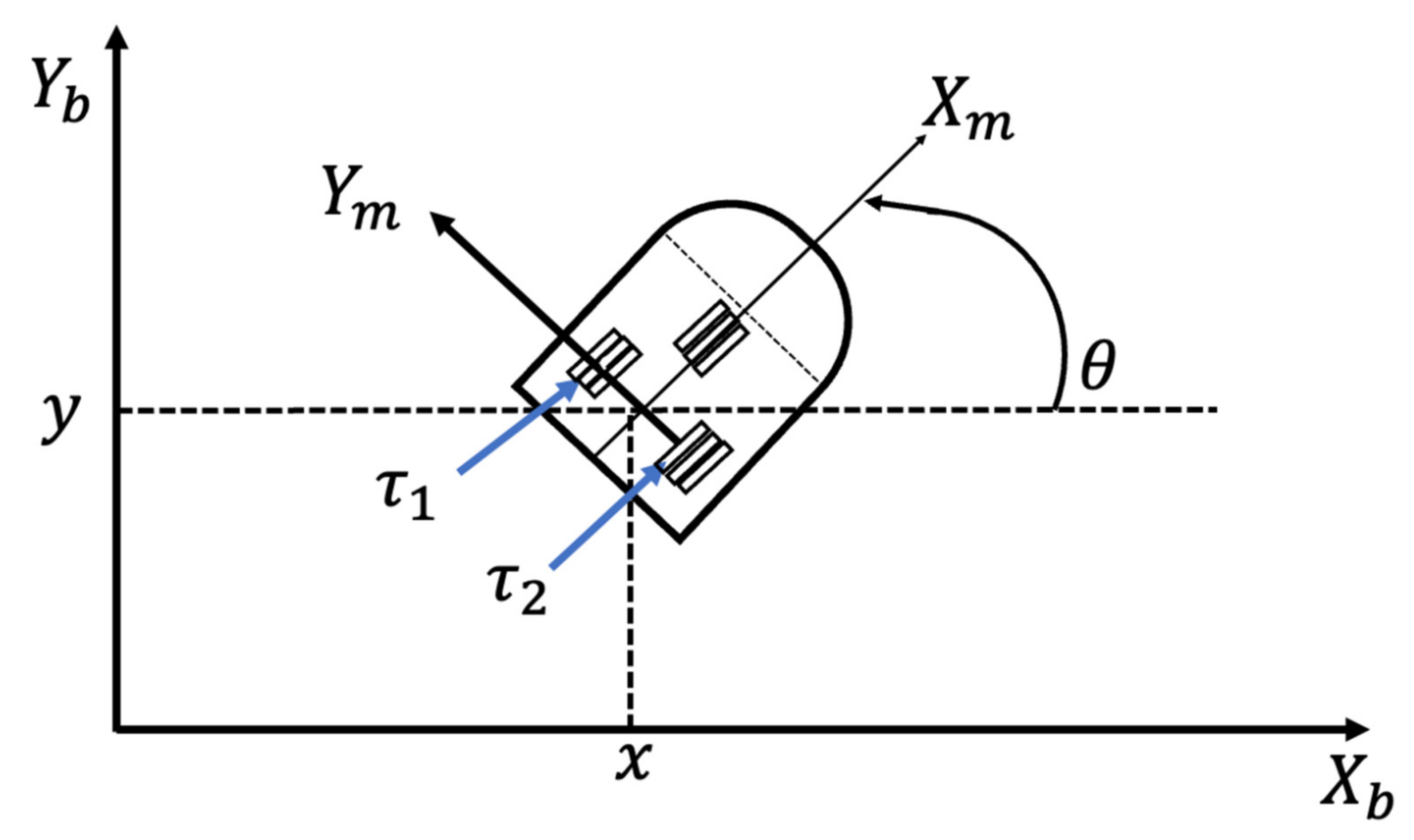
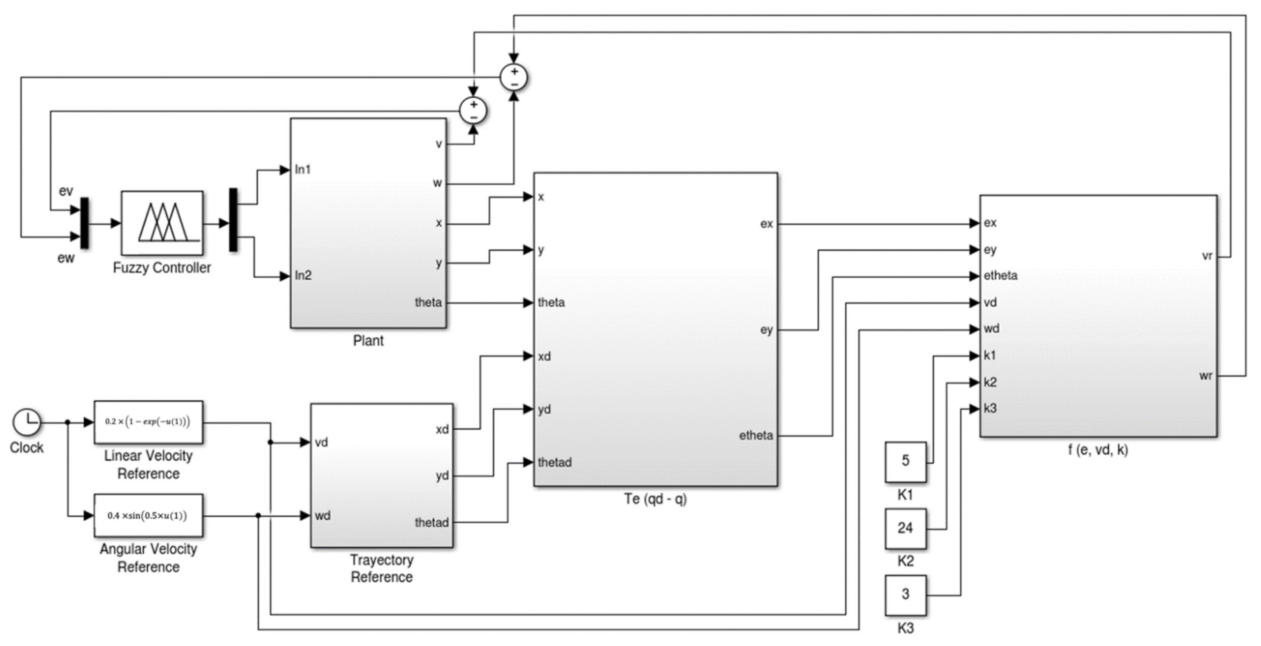
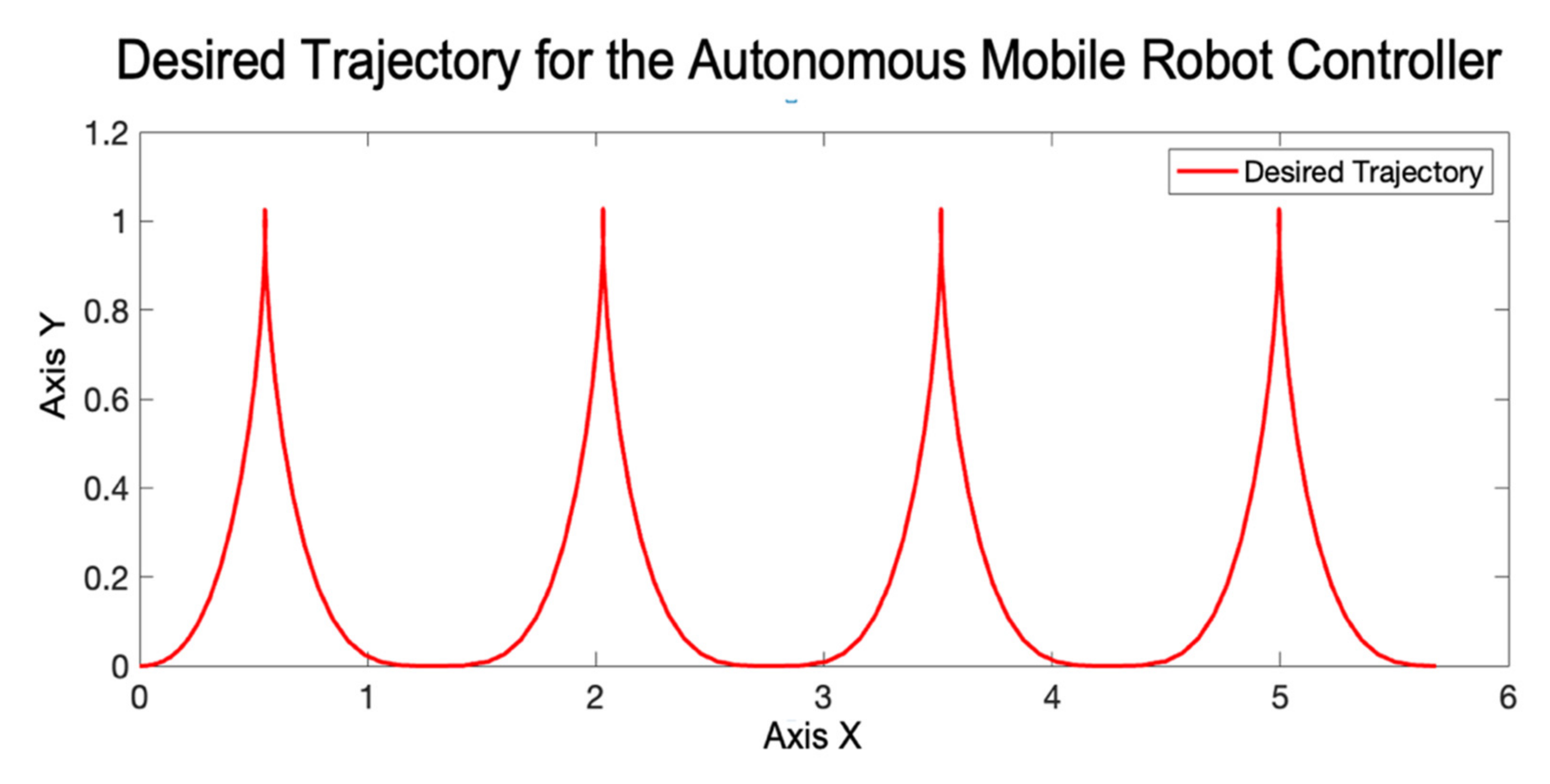
3.2. Mobile Robot Controller
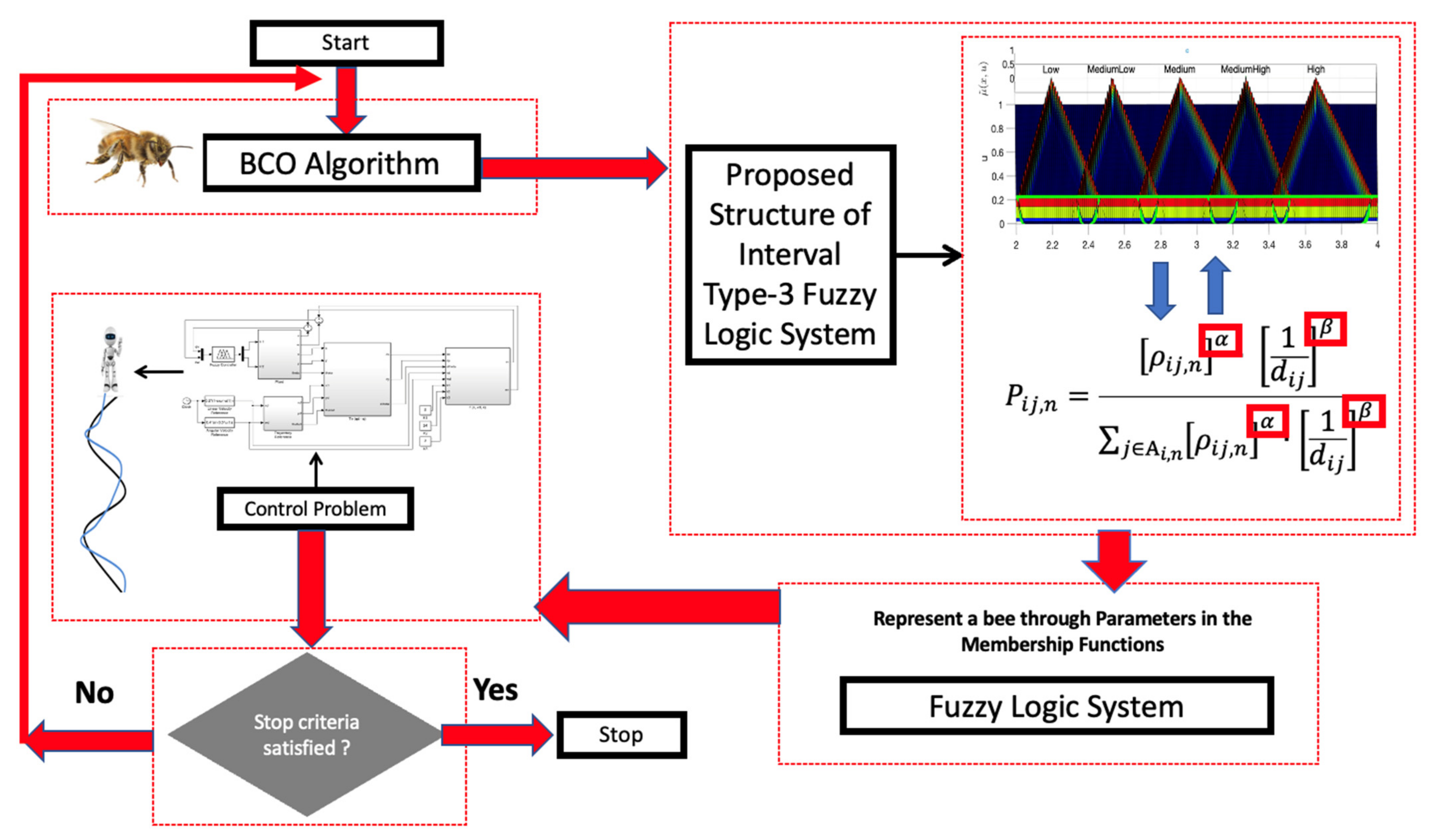
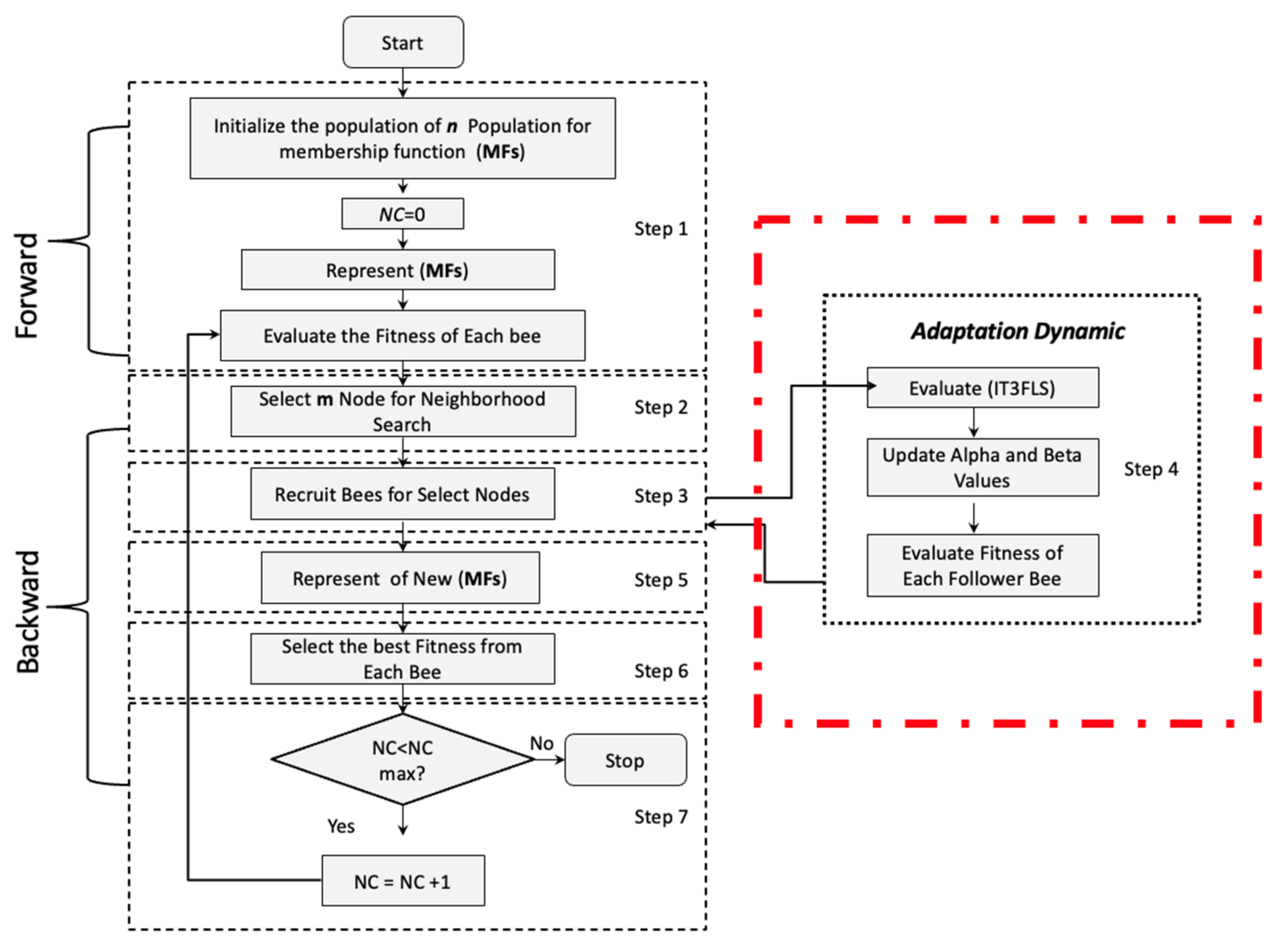
4. Fuzzy BCO
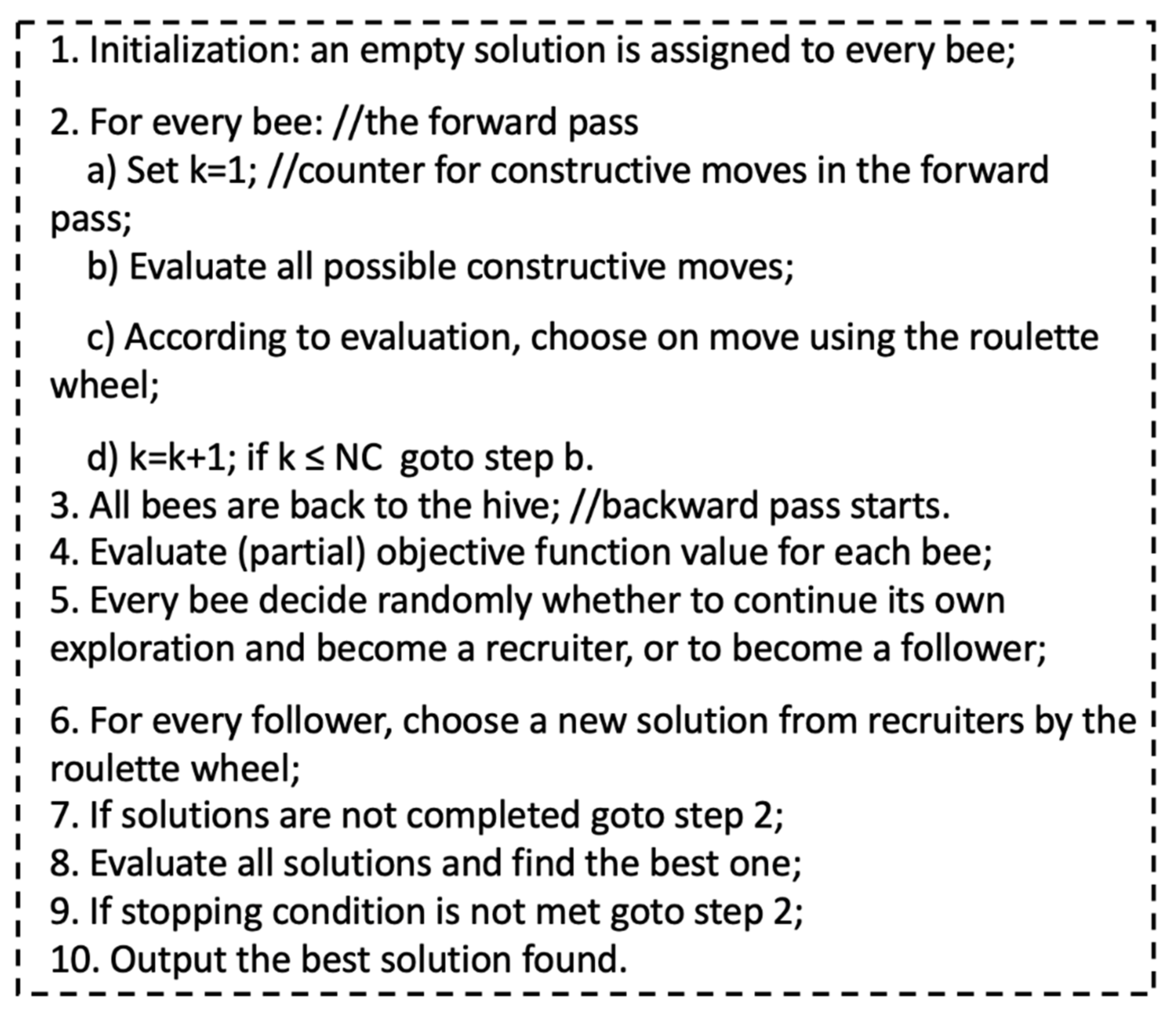
4.1. Original BCO Algorithm
4.2. Fuzzy BCO
5. Experimental Results
6. Statistical Test
7. Conclusions
Author Contributions
Funding
Acknowledgments
Conflicts of Interest
References
- Castillo, O.; Castro, J.R.; Melin, P. Interval Type-3 Fuzzy Logic Systems (IT3FLS). In Interval Type-3 Fuzzy Systems: Theory and Design; Springer: Cham, Switzerland, 2022. [Google Scholar]
- Castillo, O.; Castro, J.R.; Melin, P. A methodology for building interval type-3 fuzzy systems based on the principle of justifiable granularity. Int. J. Intell. Syst. 2022, 37, 7909–7943. [Google Scholar] [CrossRef]
- Castillo, O.; Castro, J.R.; Melin, P. Interval Type-3 Fuzzy Aggregation of Neural Networks for Multiple Time Series Prediction: The Case of Financial Forecasting. Axioms 2022, 11, 251. [Google Scholar] [CrossRef]
- Singh, D.; Verma, N.K.; Ghosh, A.K.; Malagaudanavar, A.K. An Approach Towards the Design of Interval Type-3 TS Fuzzy System. IEEE Trans. Fuzzy Syst. 2021, 30, 3880–3893. [Google Scholar] [CrossRef]
- Wang, J.H.; Tavoosi, J.; Mohammadzadeh, A.; Mobayen, S.; Asad, J.H.; Assawinchaichote, W.; Skruch, P. Non-Singleton Type-3 Fuzzy Approach for Flowmeter Fault Detection: Experimental Study in a Gas Industry. Sensors 2021, 21, 7419. [Google Scholar] [CrossRef] [PubMed]
- Alattas, K.A.; Mohammadzadeh, A.; Mobayen, S.; Aly, A.A.; Felemban, B.F. A New Data-Driven Control System for MEMSs Gyroscopes: Dynamics Estimation by Type-3 Fuzzy Systems. Micromachines 2021, 12, 1390. [Google Scholar] [CrossRef]
- Cao, Y.; Raise, A.; Mohammadzadeh, A.; Rathinasamy, S.; Band, S.S.; Mosavi, A. Deep learned recurrent type-3 fuzzy system: Application for renewable energy modeling/prediction. Energy Rep. 2021, 7, 8115–8127. [Google Scholar] [CrossRef]
- Tian, M.W.; Mohammadzadeh, A.; Tavoosi, J.; Mobayen, S.; Asad, J.H.; Castillo, O.; Várkonyi-Kóczy, A.R. A Deep-learned Type-3 Fuzzy System and Its Application in Modeling Problems. Acta Polytech. Hung. 2022, 19, 151–172. [Google Scholar] [CrossRef]
- Mohammadzadeh, A.; Sabzalian, M.H.; Zhang, W. An interval type-3 fuzzy system and a new online fractional-order learning algorithm: Theory and practice. IEEE Trans. Fuzzy Syst. 2019, 28, 1940–1950. [Google Scholar] [CrossRef]
- Ma, C.; Mohammadzadeh, A.; Turabieh, H.; Mafarja, M.; Band, S.S.; Mosavi, A. Optimal type-3 fuzzy system for solving singular multi-pantograph equations. IEEE Access 2020, 8, 225692–225702. [Google Scholar] [CrossRef]
- Balcazar, R.; Rubio, J.D.J.; Orozco, E.; Andres Cordova, D.; Ochoa, G.; Garcia, E.; Aguilar-Ibañez, C. The Regulation of an Electric Oven and an Inverted Pendulum. Symmetry 2022, 14, 759. [Google Scholar] [CrossRef]
- Rubio, J.D.J.; Orozco, E.; Cordova, D.A.; Islas, M.A.; Pacheco, J.; Gutierrez, G.J.; Mujica-Vargas, D. Modified linear technique for the controllability and observability of robotic arms. IEEE Access 2022, 10, 3366–3377. [Google Scholar] [CrossRef]
- Villaseñor Rios, C.A.; Luviano-Juárez, A.; Lozada-Castillo, N.B.; Carvajal-Gámez, B.E.; Mújica-Vargas, D.; Gutiérrez-Frías, O. Flatness-Based Active Disturbance Rejection Control for a PVTOL Aircraft System with an Inverted Pendular Load. Machines 2022, 10, 595. [Google Scholar] [CrossRef]
- Soriano, L.A.; Rubio, J.D.J.; Orozco, E.; Cordova, D.A.; Ochoa, G.; Balcazar, R.; Gutierrez, G.J. Optimization of sliding mode control to save energy in a SCARA robot. Mathematics 2021, 9, 3160. [Google Scholar] [CrossRef]
- Soriano, L.A.; Zamora, E.; Vazquez-Nicolas, J.M.; Hernández, G.; Barraza Madrigal, J.A.; Balderas, D. PD control compensation based on a cascade neural network applied to a robot manipulator. Front. Neurorobotics 2020, 14, 577749. [Google Scholar] [CrossRef]
- Silva-Ortigoza, R.; Hernández-Márquez, E.; Roldán-Caballero, A.; Tavera-Mosqueda, S.; Marciano-Melchor, M.; Garcia-Sanchez, J.R.; Silva-Ortigoza, G. Sensorless Tracking Control for a “Full-Bridge Buck Inverter–DC Motor” System: Passivity and Flatness-Based Design. IEEE Access 2021, 9, 132191–132204. [Google Scholar] [CrossRef]
- Nabipour, N.; Qasem, S.N.; Jermsittiparsert, K. Type-3 fuzzy voltage management in PV/hydrogen fuel cell/battery hybrid systems. Int. J. Hydrog. Energy 2020, 45, 32478–32492. [Google Scholar] [CrossRef]
- Liu, Z.; Mohammadzadeh, A.; Turabieh, H.; Mafarja, M.; Band, S.S.; Mosavi, A. A New Online Learned Interval Type-3 Fuzzy Control System for Solar Energy Management Systems. IEEE Access 2021, 9, 10498–10508. [Google Scholar] [CrossRef]
- Castillo, O.; Castro, J.R.; Melin, P. Interval Type-3 Fuzzy Control for Automated Tuning of Image Quality in Televisions. Axioms 2022, 11, 276. [Google Scholar] [CrossRef]
- Gheisarnejad, M.; Mohammadzadeh, A.; Farsizadeh, H.; Khooban, M.H. Stabilization of 5G telecom Converter-Based Deep Type-3 Fuzzy Machine Learning Control for Telecom Applications. IEEE Trans. Circuits Syst. II: Express Briefs 2021, 69, 544–548. [Google Scholar] [CrossRef]
- Vafaie, R.H.; Mohammadzadeh, A.; Piran, M. A new type-3 fuzzy predictive controller for MEMS gyroscopes. Nonlinear Dyn. 2021, 106, 381–403. [Google Scholar] [CrossRef]
- Mohammadzadeh, A.; Castillo, O.; Band, S.S.; Mosavi, A. A Novel Fractional-Order Multiple-Model Type-3 Fuzzy Control for Nonlinear Systems with Unmodeled Dynamics. Int. J. Fuzzy Syst. 2021, 23, 1633–1651. [Google Scholar] [CrossRef]
- Taghieh, A.; Aly, A.A.; Felemban, B.F.; Althobaiti, A.; Mohammadzadeh, A.; Bartoszewicz, A. A Hybrid Predictive Type-3 Fuzzy Control for Time-Delay Multi-Agent Systems. Electronics 2022, 11, 63. [Google Scholar] [CrossRef]
- Yan, S.; Aly, A.A.; Felemban, B.F.; Gheisarnejad, M.; Tian, M.; Khooban, M.H.; Mobayen, S. A New Event-Triggered Type-3 Fuzzy Control System for Multi-Agent Systems: Optimal Economic Efficient Approach for Actuator Activating. Electronics 2021, 10, 3122. [Google Scholar] [CrossRef]
- Gheisarnejad, M.; Mohammadzadeh, A.; Khooban, M. Model Predictive Control-Based Type-3 Fuzzy Estimator for Voltage Stabilization of DC Power Converters. IEEE Trans. Ind. Electron. 2021, 69, 13849–13858. [Google Scholar] [CrossRef]
- Tian, M.W.; Yan, S.R.; Mohammadzadeh, A.; Tavoosi, J.; Mobayen, S.; Safdar, R.; Zhilenkov, A. Stability of Interval Type-3 Fuzzy Controllers for Autonomous Vehicles. Mathematics 2021, 9, 2742. [Google Scholar] [CrossRef]
- Castillo, O. Interval type-2 fuzzy dynamic parameter adaptation in bee colony optimization for autonomous mobile robot navigation. In Recent Developments and the New Direction in Soft-Computing Foundations and Applications; Springer: Cham, Switzerland, 2021; pp. 45–62. [Google Scholar]
- Wang, H. Fuzzy control system for visual navigation of autonomous mobile robot based on Kalman filter. Int. J. Syst. Assur. Eng. Manag. 2022, 74, 1–10. [Google Scholar] [CrossRef]
- Pattnaik, S.K.; Panda, S.; Mishra, D. A multi-objective approach for local path planning of autonomous mobile robot based on metaheuristics. Concurr. Comput. Pract. Exp. 2022, 34, e6801. [Google Scholar] [CrossRef]
- Nguyen, P.T.T.; Yan, S.W.; Liao, J.F.; Kuo, C.H. Autonomous Mobile Robot Navigation in Sparse LiDAR Feature Environments. Appl. Sci. 2021, 11, 5963. [Google Scholar] [CrossRef]
- Joon, A.; Kowalczyk, W. Design of Autonomous Mobile Robot for Cleaning in the Environment with Obstacles. Appl. Sci. 2021, 11, 8076. [Google Scholar] [CrossRef]
- Jovanović, A.; Teodorović, D. Fixed-time traffic control at superstreet intersections by bee colony optimization. Transp. Res. Rec. 2022, 2676, 228–241. [Google Scholar] [CrossRef]
- Chen, R. Research on Motion Behavior and Quality-of-Life Health Promotion Strategy Based on Bee Colony Optimization. J. Healthc. Eng. 2022, 2022, 2222394. [Google Scholar] [CrossRef] [PubMed]
- Čubranić-Dobrodolac, M.; Švadlenka, L.; Čičević, S.; Trifunović, A.; Dobrodolac, M. A bee colony optimization (BCO) and type-2 fuzzy approach to measuring the impact of speed perception on motor vehicle crash involvement. Soft Comput. 2022, 26, 4463–4486. [Google Scholar] [CrossRef]
- Castillo, O.; Amador-Angulo, L. A generalized type-2 fuzzy logic approach for dynamic parameter adaptation in bee colony optimization applied to fuzzy controller design. Inf. Sci. 2018, 460, 476–496. [Google Scholar] [CrossRef]
- Cuevas, F.; Castillo, O.; Cortes-Antonio, P. Dynamic optimal parameter setting with fuzzy argument to metaheuristic algorithm variant for fuzzy tracking controllers. In Proceedings of the 2021 International Conference on Intelligent and Fuzzy Systems, Istanbul, Turkey, 24–26 August 2021; Springer: Cham, Switzerland, 2021; pp. 528–536. [Google Scholar]
- Castillo, O.; Peraza, C.; Ochoa, P.; Amador-Angulo, L.; Melin, P.; Park, Y.; Geem, Z.W. Shadowed Type-2 Fuzzy Systems for Dynamic Parameter Adaptation in Harmony Search and Differential Evolution for Optimal Design of Fuzzy Controllers. Mathematics 2021, 9, 2439. [Google Scholar] [CrossRef]
- Olivas, F.; Amador-Angulo, L.; Perez, J.; Caraveo, C.; Valdez, F.; Castillo, O. Comparative study of type-2 fuzzy particle swarm, bee colony and bat algorithms in optimization of fuzzy controllers. Algorithms 2017, 10, 101. [Google Scholar] [CrossRef]
- Amador-Angulo, L.; Mendoza, O.; Castro, J.R.; Rodríguez-Díaz, A.; Melin, P.; Castillo, O. Fuzzy sets in dynamic adaptation of parameters of a bee colony optimization for controlling the trajectory of an autonomous mobile robot. Sensors 2016, 16, 1458. [Google Scholar] [CrossRef]
- Qasem, S.N.; Ahmadian, A.; Mohammadzadeh, A.; Rathinasamy, S.; Pahlevanzadeh, B. A type-3 logic fuzzy system: Optimized by a correntropy based Kalman filter with adaptive fuzzy kernel size. Inf. Sci. 2021, 572, 424–443. [Google Scholar] [CrossRef]
- Zadeh, L.A. Fuzzy Sets. Inf. Control. 1965, 8, 338–353. [Google Scholar] [CrossRef]
- Zadeh, L.A. Fuzzy sets. In Fuzzy Sets, Fuzzy Logic, and Fuzzy Systems: Selected Papers by Lotfi A Zadeh; World Scientific: Singapore, 1996; pp. 394–432. [Google Scholar]
- Zadeh, L.A.; Klir, G.J.; Yuan, B. Fuzzy Sets, Fuzzy Logic, and Fuzzy Systems: Selected Papers; World Scientific: Singapore, 1996; Volume 6. [Google Scholar]
- Zadeh, L.A. Fuzzy Sets, Information and Control. J. Symb. Log. 1965, 8, 338–353. [Google Scholar]
- Liang, Q.; Mendel, J.M. Interval type-2 fuzzy logic systems: Theory and design. IEEE Trans. Fuzzy Syst. 2000, 8, 535–550. [Google Scholar] [CrossRef]
- Mendel, J.M.; John, R.I.; Liu, F. Interval type-2 fuzzy logic systems made simple. IEEE Trans. Fuzzy Syst. 2006, 14, 808–821. [Google Scholar] [CrossRef] [Green Version]
- Mendel, J.M.; Liu, X. Simplified interval type-2 fuzzy logic systems. IEEE Trans. Fuzzy Syst. 2013, 21, 1056–1069. [Google Scholar] [CrossRef]
- Mendel, J.M. General type-2 fuzzy logic systems made simple: A tutorial. IEEE Trans. Fuzzy Syst. 2013, 22, 1162–1182. [Google Scholar] [CrossRef]
- Lucas, L.A.; Centeno, T.M.; Delgado, M.R. General type-2 fuzzy inference systems: Analysis, design and computational aspects. In Proceedings of the 2007 IEEE International Fuzzy Systems Conference, London, UK, 23–26 July 2007; IEEE: Piscataway Township, NJ, USA, 2007; pp. 1–6. [Google Scholar]
- Mendel, J.M.; Liu, F.; Zhai, D. α -Plane Representation for Type-2 Fuzzy Sets: Theory and Applications. IEEE Trans. Fuzzy Syst. 2009, 17, 189–1207. [Google Scholar] [CrossRef]
- Mendel, J.M. Comments on alpha-plane representation for type-2 fuzzy sets: Theory and applications. IEEE Trans. Fuzzy Syst. 2010, 18, 229–230. [Google Scholar] [CrossRef]
- Castillo, O.; Castro, J.R.; Melin, P. Interval Type-3 Fuzzy Systems: Theory and Design. Stud. Fuzziness Soft Comput. 2022, 418, 1–100. [Google Scholar]
- Mendel, J.M. Uncertain Rule-Based Fuzzy Systems: Introduction and New Directions, 2nd ed.; Springer: Cham, Switzerland, 2017. [Google Scholar]
- Karnik, N.N.; Mendel, J.M. Operations on Type-2 Fuzzy Sets. Fuzzy Sets Syst. 2001, 122, 327–348. [Google Scholar] [CrossRef]
- Sakalli, A.; Kumbasar, T.; Mendel, J.M. Towards Systematic Design of General Type-2 Fuzzy Logic Controllers: Analysis, Interpretation, and Tuning. IEEE Trans. Fuzzy Syst. 2021, 29, 226–239. [Google Scholar] [CrossRef]
- Karnik, N.N.; Mendel, J.; Liang, Q. Type-2 fuzzy logic systems. IEEE Trans. Fuzzy Syst. 1999, 7, 643–658. [Google Scholar] [CrossRef]
- Mendel, J.M. Enhanced Karnik—Mendel Algorithms. IEEE Trans. Fuzzy Syst. 2009, 17, 923–934. [Google Scholar]
- Iancu, I. A Mamdani type fuzzy logic controller. Fuzzy Log. Control. Concepts Theor. Appl. 2012, 15, 325–350. [Google Scholar]
- Mamdani, E.H. Application of fuzzy algorithms for control of simple dynamic plant. In Proceedings of the Institution of electrical Engineers; IET: London, UK, 1974; Volume 121, pp. 1585–1588. [Google Scholar]
- Calcev, G. Some remarks on the stability of Mamdani fuzzy control systems. IEEE Trans. Fuzzy Syst. 1998, 6, 436–442. [Google Scholar] [CrossRef]
- Mamdani, E.H. Application of fuzzy logic to approximate reasoning using linguistic synthesis. IEEE Trans. Comput. 1977, 26, 1182–1191. [Google Scholar] [CrossRef]
- Mamdani, E.H.; Assilian, S. An experiment in linguistic synthesis with a fuzzy logic controller. Int. J. Man-Mach. Stud. 1975, 7, 1–13. [Google Scholar] [CrossRef]
- Teodorović, D. Bee colony optimization (BCO). In Innovations in Swarm Intelligence; Springer: Berlin/Heidelberg, Germany, 2009; pp. 39–60. [Google Scholar]
- Teodorović, D. Transport Modeling by Multi-Agent Systems: A Swarm Intelligence Approach. Transp. Plan. Technol. 2003, 26, 289–312. [Google Scholar] [CrossRef]
- Teodorović, D. Swarm Intelligence Systems for Transportation Engineering: Principles and Applications. Transp. Res. Part. C Emerg. Technol. 2008, 16, 651–782. [Google Scholar] [CrossRef]
- Wong, L.P.; Low, M.Y.H.; Chong, C.S. A bee colony optimization algorithm for traveling salesman problem. In Proceedings of the 2008 Second Asia International Conference on Modelling & Simulation (AMS), Washington, DC, USA, 13–15 May 2008; IEEE: Piscataway Township, NJ, USA, 2008; pp. 818–823. [Google Scholar]


| Performance Inde× | Methods | |||||
|---|---|---|---|---|---|---|
| Original BCO | FBCO-T1FLS | FBCO-IT2FLS | FBCO-GT2FLS | FBCO-IT3FLS | ||
| ITAE | 1.94 × 10+3 | 1.97 × 10+3 | 1.95 × 10+3 | 1.96 × 10+3 | 1.96 × 10+3 | |
| ITSE | 7.81 × 10+2 | 8.03 × 10+2 | 7.80 × 10+2 | 7.91 × 10+2 | 7.87 × 10+2 | |
| IAE | 3.92 × 10+1 | 3.98 × 10+1 | 3.94 × 10+1 | 3.96 × 10+1 | 3.96 × 10+1 | |
| ISE | 1.59 × 10+1 | 1.63 × 10+1 | 1.59 × 10+1 | 1.60 × 10+1 | 1.60 × 10+1 | |
| MSE | 3.27 × 100 | 1.31 × 100 | 9.83 × 10⁻¹ | 1.46 × 100 | 1.19 × 100 | |
| RMSE | 1.60 × 100 | 1.75 × 100 | 1.73 × 100 | 1.52 × 100 | 1.67 × 100 | |
| MSE | Std. | 2.08 × 100 | 2.10 × 100 | 1.15 × 100 | 3.46 × 100 | 1.79 × 100 |
| Best | 8.99 × 10⁻³ | 1.03 × 10⁻² | 1.03 × 10⁻² | 1.03 × 10⁻² | 1.34 × 10⁻² | |
| Worst | 1.05 × 10+1 | 7.72 × 100 | 3.77 × 100 | 1.82 × 10+1 | 6.58 × 100 | |
| Beta | 3 (Fixed) | 3.625 | 2.599 | 2.478 | 2.734 | |
| Alpha | 0.5 (Fixed) | 0.818 | 0.466 | 0.456 | 0.555 | |
| Performance Inde× | Methods | |||||
|---|---|---|---|---|---|---|
| Original BCO | FBCO-T1FLS | FBCO-IT2FLS | FBCO-GT2FLS | FBCO-IT3FLS | ||
| ITAE | 1.96 × 10+3 | 1.97 × 10+3 | 1.97 × 10+3 | 1.96 × 10+3 | 1.95 × 10+3 | |
| ITSE | 7.93 × 10+2 | 7.96 × 10+2 | 7.94 × 10+2 | 7.88 × 10+2 | 7.91 × 10+2 | |
| IAE | 3.96 × 10+1 | 3.97 × 10+1 | 3.97 × 10+1 | 3.96 × 10+1 | 3.94 × 10+1 | |
| ISE | 1.16 × 10+1 | 1.61 × 10+1 | 1.61 × 10+1 | 1.60 × 10+1 | 1.60 × 10+1 | |
| MSE | 9.93 × 10⁻¹ | 9.34 × 10⁻¹ | 2.16 × 100 | 1.40 × 100 | 1.00 × 100 | |
| RMSE | 1.54 × 100 | 1.33 × 100 | 1.72 × 100 | 1.59 × 100 | 1.53 × 100 | |
| MSE | Std. | 1.78 × 100 | 1.83 × 100 | 4.65 × 100 | 3.35 × 100 | 1.44 × 100 |
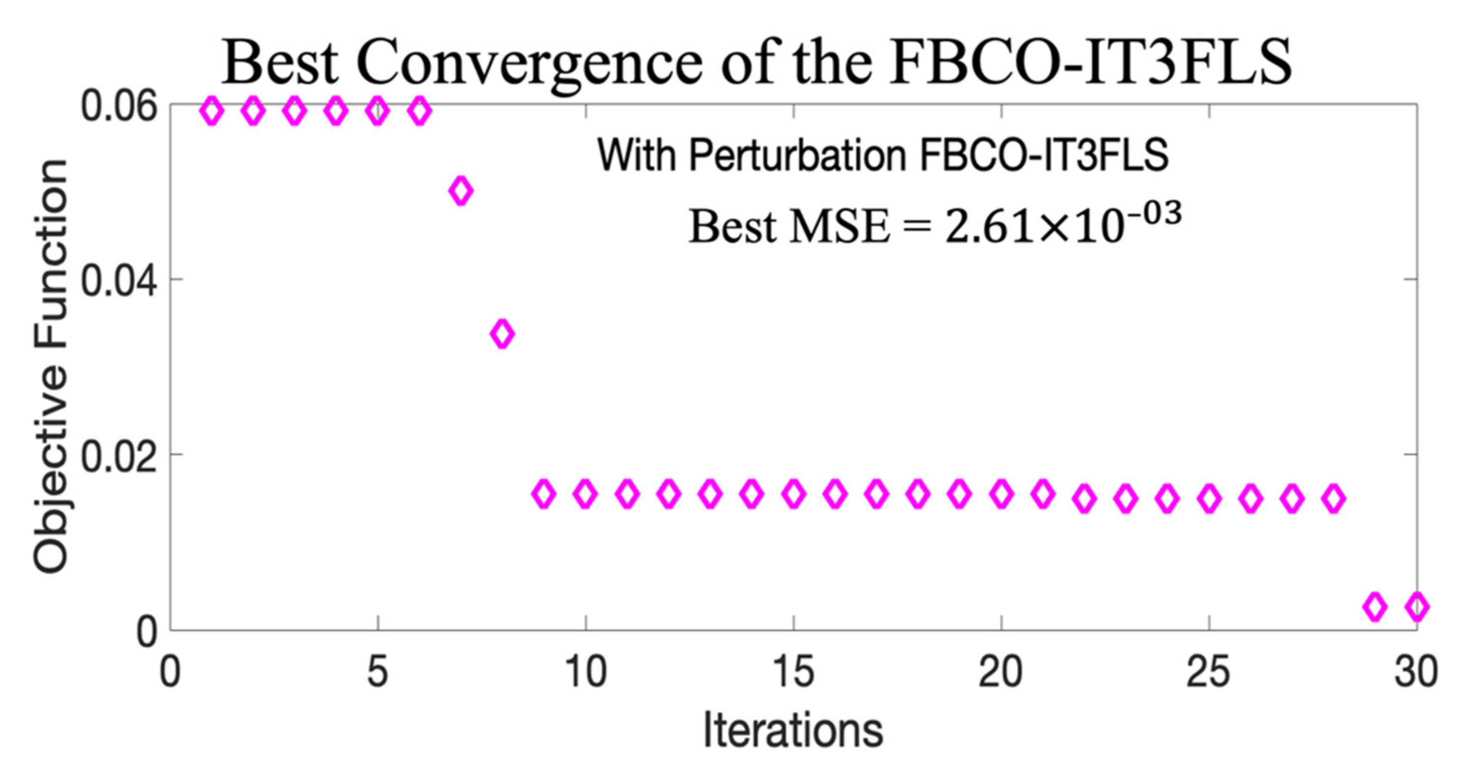
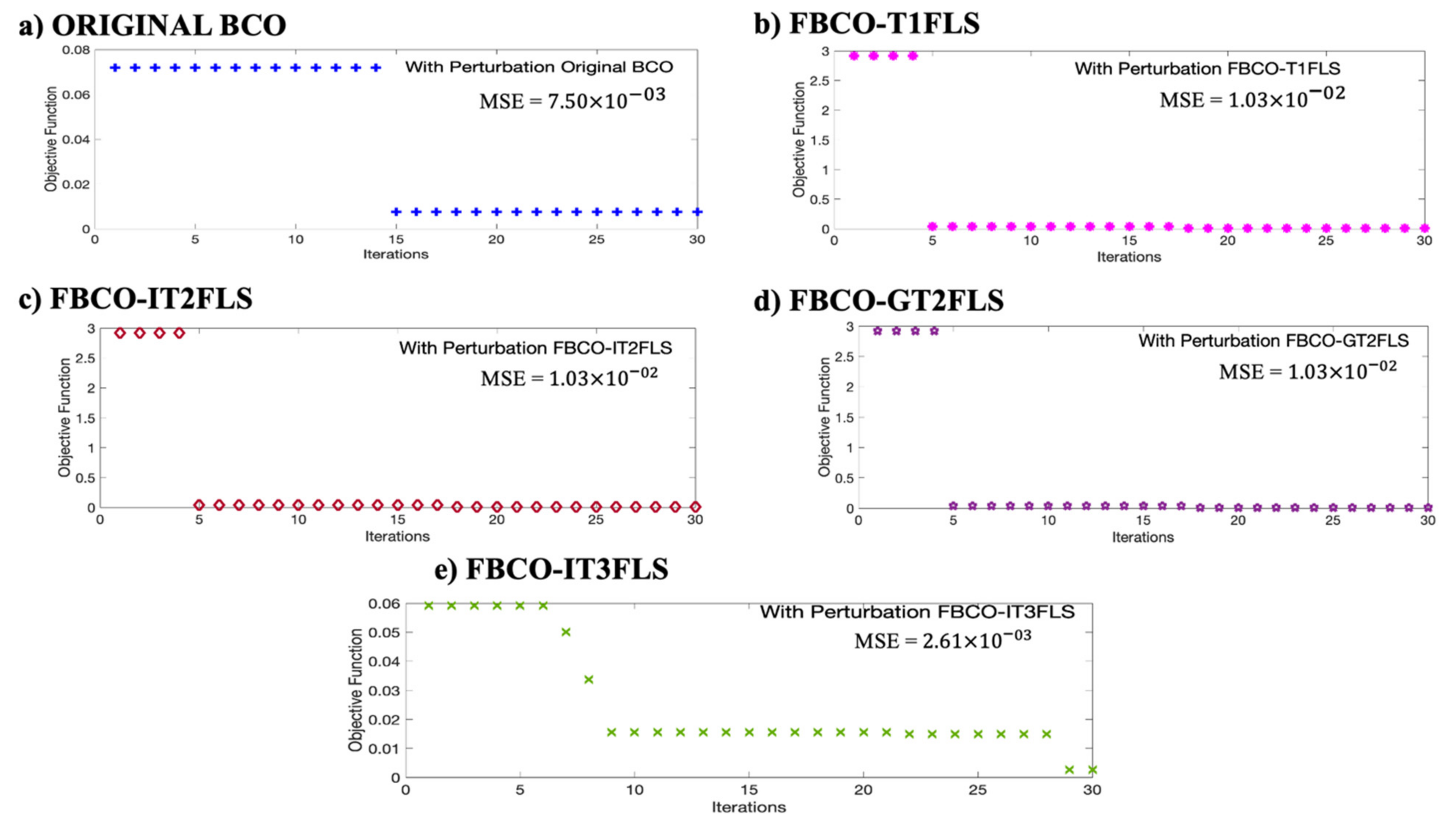
| Best | 7.53 × 10⁻³ | 1.03 × 10⁻² | 1.03 × 10⁻² | 1.03 × 10⁻² | 2.61 × 10⁻³ | |
| Worst | 6.00 × 100 | 7.72 × 100 | 1.83 × 10+1 | 1.82 × 10+1 | 4.46 × 100 | |
| Beta | 3 (Fixed) | 3.625 | 2.640 | 2.568 | 2.602 | |
| Alpha | 0.5 (Fixed) | 0.818 | 0.530 | 0.486 | 0.487 | |
| Experiment | FBCO-T1FLS | FBCO-IT2FLS | FBCO-GT2FLS | FBCO-IT3FLS | ||||
|---|---|---|---|---|---|---|---|---|
| 1 | 3.626 | 0.818 | 2.812 | 0.570 | 3.021 | 0.456 | 2.645 | 0.510 |
| 2 | 3.287 | 0.742 | 2.604 | 0.469 | 2.973 | 0.487 | 2.571 | 0.472 |
| 3 | 3.625 | 0.818 | 2.623 | 0.476 | 2.881 | 0.505 | 3.277 | 0.831 |
| 4 | 3.625 | 0.818 | 2.599 | 0.466 | 2.881 | 0.505 | 2.572 | 0.472 |
| 5 | 3.287 | 0.742 | 2.941 | 0.643 | 2.973 | 0.487 | 3.277 | 0.832 |
| 6 | 3.625 | 0.818 | 2.599 | 0.465 | 2.973 | 0.487 | 2.816 | 0.599 |
| 7 | 3.625 | 0.818 | 3.010 | 0.635 | 2.973 | 0.487 | 2.572 | 0.472 |
| 8 | 3.625 | 0.818 | 2.640 | 0.530 | 3.021 | 0.456 | 2.816 | 0.599 |
| 9 | 3.287 | 0.742 | 2.640 | 0.530 | 3.021 | 0.456 | 3.277 | 0.832 |
| 10 | 3.287 | 0.742 | 2.640 | 0.530 | 2.881 | 0.505 | 2.571 | 0.472 |
| 11 | 3.625 | 0.818 | 2.640 | 0.530 | 2.881 | 0.505 | 2.570 | 0.472 |
| 12 | 3.625 | 0.818 | 2.640 | 0.530 | 2.973 | 0.487 | 2.572 | 0.472 |
| 13 | 3.625 | 0.818 | 2.640 | 0.530 | 2.881 | 0.505 | 2.624 | 0.499 |
| 14 | 3.625 | 0.818 | 2.640 | 0.530 | 3.021 | 0.456 | 2.794 | 0.588 |
| 15 | 3.625 | 0.818 | 2.640 | 0.530 | 2.881 | 0.505 | 2.642 | 0.509 |
| 16 | 3.625 | 0.818 | 2.640 | 0.530 | 3.021 | 0.456 | 2.572 | 0.472 |
| 17 | 3.625 | 0.818 | 3.010 | 0.635 | 2.881 | 0.505 | 2.906 | 0.645 |
| 18 | 3.625 | 0.818 | 2.640 | 0.530 | 2.973 | 0.487 | 2.572 | 0.472 |
| 19 | 3.625 | 0.818 | 3.010 | 0.635 | 2.973 | 0.487 | 2.570 | 0.471 |
| 20 | 3.287 | 0.742 | 2.640 | 0.530 | 2.881 | 0.505 | 2.655 | 0.521 |
| 21 | 3.625 | 0.818 | 2.640 | 0.530 | 2.973 | 0.487 | 2.602 | 0.488 |
| 22 | 3.625 | 0.818 | 2.640 | 0.530 | 2.881 | 0.505 | 2.593 | 0.483 |
| 23 | 3.625 | 0.818 | 2.640 | 0.530 | 2.881 | 0.505 | 2.793 | 0.587 |
| 24 | 3.625 | 0.818 | 2.640 | 0.530 | 2.973 | 0.487 | 2.629 | 0.502 |
| 25 | 3.625 | 0.818 | 2.640 | 0.530 | 2.881 | 0.505 | 2.774 | 0.578 |
| 26 | 3.625 | 0.818 | 2.640 | 0.530 | 3.021 | 0.456 | 2.644 | 0.510 |
| 27 | 3.625 | 0.818 | 2.640 | 0.530 | 3.021 | 0.456 | 2.605 | 0.489 |
| 28 | 3.625 | 0.818 | 2.640 | 0.530 | 3.021 | 0.456 | 3.277 | 0.832 |
| 29 | 3.625 | 0.818 | 3.010 | 0.635 | 2.973 | 0.487 | 2.718 | 0.548 |
| 30 | 3.287 | 0.742 | 2.640 | 0.530 | 2.973 | 0.487 | 3.277 | 0.832 |
| AVERAGE | 3.558 | 0.803 | 2.703 | 0.541 | 2.952 | 0.485 | 2.760 | 0.569 |
| Method | FBCO-IT3FLS | Original BCO | FBCO-T1FLS | FBCO-IT2FLS | FBCO-GT2FLS |
|---|---|---|---|---|---|
| Minimun | 1.34 ×10⁻² | 8.99 × 10⁻³ | 1.03 × 10⁻² | 1.03 × 10⁻² | 1.03 × 10⁻² |
| Maximum | 6.58 × 100 | 1.05 × 10+1 | 7.72 × 100 | 3.77 × 100 | 1.82 × 10+1 |
| Average | 1.19 × 100 | 1.12 × 100 | 1.31 × 100 | 9.83 × 10⁻¹ | 1.46 × 100 |
| Std. | 1.79 × 100 | 2.08 × 100 | 2.10 × 100 | 1.15 × 100 | 3.46 × 100 |
| Z Value | −4.6307 | −1.4274 | −1.4274 | −1.4274 | |
| Evidence | Significative | Not Significative | Not Significative | Not Significative |
| Method | FBCO-IT3FLS | Original BCO | FBCO-T1FLS | FBCO-IT2FLS | FBCO-GT2FLS |
|---|---|---|---|---|---|
| Minimun | 2.61 × 10⁻³ | 7.53 × 10⁻³ | 1.03 × 10⁻² | 1.03 × 10⁻² | 1.03 × 10⁻² |
| Maximum | 4.46 × 100 | 6.00 × 100 | 7.72 × 100 | 1.83 × 10+1 | 1.82 × 10+1 |
| Average | 1.00 × 100 | 9.93 × 10⁻¹ | 9.34 × 10⁻¹ | 2.16 × 100 | 1.40 × 100 |
| Std. | 1.44 × 100 | 1.78 × 100 | 1.83 × 100 | 4.65 × 100 | 3.35 × 100 |
| Z Value | −1.8109 | −2.1111 | −2.1111 | −2.1111 | |
| Evidence | Significative | Significative | Significative | Significative |
Publisher’s Note: MDPI stays neutral with regard to jurisdictional claims in published maps and institutional affiliations. |
© 2022 by the authors. Licensee MDPI, Basel, Switzerland. This article is an open access article distributed under the terms and conditions of the Creative Commons Attribution (CC BY) license (https://creativecommons.org/licenses/by/4.0/).
Share and Cite
Amador-Angulo, L.; Castillo, O.; Melin, P.; Castro, J.R. Interval Type-3 Fuzzy Adaptation of the Bee Colony Optimization Algorithm for Optimal Fuzzy Control of an Autonomous Mobile Robot. Micromachines 2022, 13, 1490. https://doi.org/10.3390/mi13091490
Amador-Angulo L, Castillo O, Melin P, Castro JR. Interval Type-3 Fuzzy Adaptation of the Bee Colony Optimization Algorithm for Optimal Fuzzy Control of an Autonomous Mobile Robot. Micromachines. 2022; 13(9):1490. https://doi.org/10.3390/mi13091490
Chicago/Turabian StyleAmador-Angulo, Leticia, Oscar Castillo, Patricia Melin, and Juan R. Castro. 2022. "Interval Type-3 Fuzzy Adaptation of the Bee Colony Optimization Algorithm for Optimal Fuzzy Control of an Autonomous Mobile Robot" Micromachines 13, no. 9: 1490. https://doi.org/10.3390/mi13091490
APA StyleAmador-Angulo, L., Castillo, O., Melin, P., & Castro, J. R. (2022). Interval Type-3 Fuzzy Adaptation of the Bee Colony Optimization Algorithm for Optimal Fuzzy Control of an Autonomous Mobile Robot. Micromachines, 13(9), 1490. https://doi.org/10.3390/mi13091490