Article

Milling Stability Prediction: A New Approach Based on a Composited Newton–Cotes Formula

1
School of Mechanical Engineering, Hefei University of Technology, Hefei 230009, China
2
School of Mechanical Engineering, Hangzhou Dianzi University, Hangzhou 310018, China
3
School of Mechanical Engineering, Zhejiang Sci-Tech University, Hangzhou 310018, China
*
Author to whom correspondence should be addressed.
Micromachines 2023, 14(7), 1304; https://doi.org/10.3390/mi14071304
Submission received: 5 June 2023 / Revised: 20 June 2023 / Accepted: 21 June 2023 / Published: 25 June 2023

Abstract

:
Based on a composited Newton–Cotes formula, this paper proposes a numerical method to predict milling stability considering regenerative chatter and focusing on rate and prediction accuracy. First, the dynamic model of milling motion is expressed as state-space equations considering regenerative chatter, with the tooth passing period divided into a set of time intervals. Second, a composited Newton–Cotes formula is introduced to calculate the transition function map for each time interval. Third, the state transition matrix is constructed based on the above-mentioned transition function, and the prediction stability boundary is determined by the Floquet theory. Finally, simulation analysis and experimental verification are conducted to verify the effectiveness of the proposed method. The simulation results demonstrate that, for the milling model with a single degree of freedom (DOF), the convergence rate and prediction accuracy of the proposed method are higher than those of the comparison method. The experimental results demonstrate that, for the milling model with two DOFs, the machining parameters below the prediction stability boundary can avoid the chatter as much as possible, ensuring the machined surface quality.

1. Introduction

Regenerative chatter arising from a self-excitation chatter vibration may be unavoidable in milling processes, which will reduce machining quality and efficiency and accelerate tool wear [1,2]. Researchers have attempted to avoid regenerative chatter using prediction [3,4], identification [5,6,7], and suppression [8,9,10] methods. The research results demonstrate that selecting machining parameters to avoid chatter occurrence is vital and that the stability lobe diagrams provide a reference for appropriately selecting machining parameters [11]. The objective of this study is to develop a method to draw stability lobe diagrams with high precision.
As regenerative chatter is integrated into the dynamics model, the dynamics model is reformulated as delay differential equations (DDEs) with time-periodic coefficients [12,13]. So far, many methods, including experimental, analytical, and numerical methods, have been proposed to solve the DDEs to obtain stability lobe diagrams. Based on the zeroth-order harmonics of the Fourier series expansion, Altintas et al. [14] transformed the DDEs into the Laplace frequency, which is more suitable for high-radical-immersion milling. Taking higher-order harmonics into account, Merdol et al. [15] proposed a multi-frequency solution for low-radical-immersion milling, which is also called the multi-frequency method. In addition to the above-mentioned stability analysis methods in the frequency domain, there are some stability analysis methods in the time domain. Insperger et al. [16,17] first presented a semi-discretization method (SDM) for a delayed system and then presented an updated version of the SDM (first-order SDM) for periodic systems with a single discrete time delay. By extending the SDM and first-order SDM, the second-order SDM (second-order SDM) has also been proposed for variable spindle speed milling [18]. Ding et al. [19] proposed a full-discretization method (FDM) in virtue of a direct integration scheme. To further improve the prediction accuracy, Ding et al. [20] and Yan et al. [21] presented the second-order FDM and third-order FDM, respectively. Based on the integral equation and numerical integration formulas, Ding et al. [22] developed a concise semi-analytical method for constructing a discrete dynamical map approximating the DDEs. Dong et al. [23] have recently proposed an updated numerical integration method. Li et al. [24] proposed an accurate and fast milling stability prediction approach based on the Newton–Cotes method (NCM). In addition to the above-mentioned methods, other methods such as the Adams–Moulton-based method [25], the spectral element method [26], and the Lyapunov–Krasovskii method [27] exist. The aforementioned stability analysis methods mainly focus on three targets: convergence rate, prediction accuracy, and computational efficiency. These three targets usually contradict each other to a certain extent. Based on a composited Newton–Cotes formula, this paper presents a novel milling stability prediction method, i.e., the composited Newton–Cotes method (CNCM), with a high convergence rate and prediction accuracy.
The remainder of this paper is organized as follows. Section 2 provides a brief description of the composited Newton–Cotes formula. The composited Newton–Cotes-based milling stability analysis method is presented in Section 3. Comparisons of the convergence rate, prediction accuracy, and computational efficiency between the proposed method and NCM are presented in Section 4, and experimental verification is presented in Section 5. Finally, conclusions are drawn in Section 6.

2. Composited Newton–Cotes Formula

The nth-order Newton–Cotes formula has at least n-order algebraic accuracy [28], which is defined as
a b f t d t = b a k = 0 n C k n f x k
where [a, b] denotes the parameter interval, and it is divided into n equal intervals. The span of each interval is defined as b a / n , and then x k = a + k b a / n is deduced. The C k n denotes the cotes coefficient and is defined as
C k n = 1 n k n k ! n k 0 n j = 0 , j k n τ j d τ k = 0 , 1 , , n ,
where depends only on n. It is worth mentioning that the approximation accuracy of Equation (1) is significantly reduced when n is greater than or equal to eight. Increasing n cannot ensure the approximation accuracy of Equation (1). To this end, the composited Newton–Cotes formula is introduced below. To improve the integration accuracy, mid-points of the interval should be considered. So the interval x k , x k + 1 is divided into four equal sub-intervals: x k , x k + 1 / 4 , x k + 1 / 2 , x k + 3 / 4 , and x k + 1 . The lower-order Newton–Cotes formula is used in each sub-interval, and then the approximation results of each subinterval are finally added together. According to Bool’s rule (n = 4), the fourth-order composited Newton–Cotes formula [29] can be introduced as follows:
a b f t d t = 7 Δ 90 f a + k = 0 n 1 f x k + k = 0 n 1 f x k + 1 + f b + 16 Δ 45 k = 0 n 1 f x k + 1 / 4 + k = 0 n 1 f x k + 3 / 4 + 2 Δ 15 k = 0 n 1 f x k + 1 / 2
where Δ = b a / n . The remainder of the equation above is
R n = 2 b a 945 Δ 4 6 f 6 u u a , b .

3. Mathematical Model

In this work, it is assumed that the workpiece is rigid, that the milling cutters have two DOFs and that there is no tool run-out situation in the milling process. The tool helix angle is not considered either. Considering the regenerative chatter, the mathematical model of milling motion can be formulated as a second-order differential Equation (24) as follows:
M q ¨ t + C q ˙ t + K q t = a p K C T q t q t T ,
where M, C, and K denote the modal stiffness, mass, and damping matrices of the milling system, respectively; q t denotes the displacement vector, q ˙ t and q ¨ t denote its first- and second-order derivatives with respect to t; a p denotes the depth of cut; K C t is a time-periodic coefficient matrix that satisfies K C t = K C t + T ; T denotes the time delay. For the milling cutter, it is the same as one-tooth passing period, i.e., T = 60 / N Ω , where N denotes the number of tool teeth and Ω denotes the spindle speed (rpm).
A new vector x t as x t = q t , q ˙ t T is defined, and then the state-space expression of (5), can be expressed as [22]
x ˙ t = A x t + a p B t x t x t T
where
A = 0 I M 1 K M 1 C
B t = 0 0 M 1 K C t 0
K C t = h x x t 0 0 0
h x x t = j = 1 N g ϕ j t sin ϕ j t K t cos ϕ j t + K n sin ϕ j t
where K t and K n denote the tangential and normal linearised cutting force coefficients, respectively. The ϕ j t denotes the angular position of the jth tooth.
Based on the Volterra integral equation of the second type [30], the analytical expression of (6) is deduced as follows:
x t = e A t t s t x t s t + a p t s t t e A t ξ B ξ x ξ x ξ T d ξ
where t s t is the starting time of the computation.
Depending on whether the cutter touches the workpiece, the vibrations can be classified into free and excited vibration process [31]. If the cutter is not in contact with the workpiece, the vibrations are free vibration processes, which are equivalent to B t = 0 . Then, Equation (11), can be simplified as
x t = e A t f x t s t
where t f is the free vibration cycle.
If the cutter is in contact with the workpiece, the vibrations are excited vibration processes. The corresponding cycle t i is
t i = t s t + t f + i 1 h
where i = 2 m m = 0 , 1 , 2 , , ceil n / 2 1 , where ceil ( · ) is a function that rounds positive numbers to plus infinity) and h = T t f / n .
By substituting Equation (13), into Equation (11), we obtain
x t i + 1 = e A t i + 1 t i x t i + a p t i t i + 1 e A t i + 1 ξ B ξ x ξ x ξ T d ξ
Based on the composite Newton–Cotes formula introduced in Section 2, if the time interval t i , t i + 1 is divided into four equal sub-intervals, that is, t i , t i + 1 / 4 , t i + 1 / 2 , t i + 3 / 4 , and t i + 1 , then the state items x t i + 1 / 4 , x t i + 1 / 2 , and x t i + 3 / 4 can be approximated as follows:
x t i + 1 / 4 21 x t i + 14 x t i + 1 3 x t i + 2 32 ,
x t i + 1 / 2 3 x t i + 6 x t i + 1 x t i + 2 8 ,
x t i + 3 / 4 5 x t i + 30 x t i + 1 3 x t i + 2 32 .
To simplify the process, several abbreviated expressions are used as below. Let
x i = x t i
B i = B t i
σ t , ξ , x ξ = a p e A t ξ B ξ x ξ x ξ T
By combining Equations (15)–(20), x t i + 1 can be computed by
x i + 1 = e A h x i + h 90 7 σ t i + 1 , t i , x i + σ t i + 1 , t i + 1 , x i + 1 + 12 σ t i + 1 , t i + 1 / 2 , 3 x i + 6 x i + 1 x i + 2 8 + 32 σ t i + 1 , t i + 1 / 4 , 21 x i + 14 x i + 1 3 x i + 2 32 + σ t i + 1 , t i + 3 / 4 , 5 x i + 30 x i + 1 3 x i + 2 32
On this basis, we utilise Simpson’s rule to calculate x i + 2 :
x i + 2 = e 2 A h x i + a p h 3 e 2 A h B i x i x i + T + 4 e A h B i + 1 x i + 1 x i + 1 T + B i + 2 x i + 2 x i + 2 T .
By combining Equations (21) and (22), we can obtain general iterative algorithms, and the state transition equations can be written as
F i x i + F i + 1 x i + 1 + F i + 2 x i + 2 = F i T x i T + F i + 1 T x i + 1 T + F i + 2 T x i + 2 T
G i x i + G i + 1 x i + 1 + G i + 2 x i + 2 = G i T x i T + G i + 1 T x i + 1 T + G i + 2 T x i + 2 T
where
F i = e A h a p h 180 14 e A h B i + 42 e 3 A h / 4 B i + 1 / 4 + 9 e A h / 2 B i + 1 / 2 + 10 e A h / 4 B i + 3 / 4
F i + 1 = I a p h 90 7 e A h B i + 1 + 14 e 3 A h / 4 B i + 1 / 4 + 9 e A h / 2 B i + 1 / 2 + 30 e A h / 4 B i + 3 / 4
F i + 2 = a p h 60 2 e 3 A h / 4 B i + 1 / 4 + e A h / 2 B i + 1 / 2 + 2 e A h / 4 B i + 3 / 4
F i T = a p h 180 14 e A h B i + 42 e 3 A h / 4 B i + 1 / 4 + 9 e A h / 2 B i + 1 / 2 + 10 e A h / 4 B i + 3 / 4
F i + 1 T = a p h 90 7 e A h B i + 1 + 14 e 3 A h / 4 B i + 1 / 4 + 9 e A h / 2 B i + 1 / 2 + 30 e A h / 4 B i + 3 / 4
F i + 2 T = a p h 60 2 e 3 A h / 4 B i + 1 / 4 + e A h / 2 B i + 1 / 2 + 2 e A h / 4 B i + 3 / 4
G i = e 2 A h a p h 3 e 2 A h B i
G i + 1 = 4 a p h 3 e A h B i + 1
G i + 2 = I a p h 3 B i + 2
G i T = a p h 3 e 2 A h B i
G i + 1 T = 4 a p h 3 e A h B i + 1
G i + 2 T = a p h 3 B i + 2
where I is the identity matrix.
After solving the equations above, the state transition matrix is established as follows:
I P a p h 90 Q x t 0 x t 1 x t n + 2 = R a p h 90 Q x t 0 T x t 1 T x t n + 2 T
where
P = 0 0 0 0 0 0 e A h 0 0 0 0 0 e 2 A h 0 0 0 0 0 0 0 0 0 0 0 0 0 0 e A h 0 0 0 0 0 e 2 A h 0 0 2 n + 2 × 2 n + 2
Q = 0 0 0 0 0 0 α 0 α 1 α 2 0 0 0 β 0 β 1 β 2 0 0 0 0 0 0 β i 0 0 0 0 0 α i α i + 1 α i + 2 0 0 0 β i β i + 1 β i + 2 2 n + 2 × 2 n + 2
R = 0 0 0 0 0 e A h 0 0 0 0 0 0 0 0 0 0 0 0 0 0 0 0 0 0 0 0 0 0 0 0 0 0 0 0 0 0 2 n × 2 × 2 n + 2
where
α i = 7 e A h B i + 21 e 3 A h / 4 B i + 1 / 4 + 9 2 e A h / 2 B i + 1 / 2 + 5 e A h / 4 B i + 3 / 4
α i + 1 = 7 e A h B i + 1 + 14 e 3 A h / 4 B i + 1 / 4 + 9 e A h / 2 B i + 1 / 2 + 30 e A h / 4 B i + 3 / 4
α i + 2 = 30 e 3 A h / 4 B i + 1 / 4 3 2 e A h / 2 B i + 1 / 2 3 e A h / 4 B i + 3 / 4
β i = 30 e 2 A h B i
β i + 1 = 120 e A h B i + 1
β i + 2 = 30 B i + 2
The state transition matrix of the one tooth passing period is expressed as
Φ = I P a p h 90 Q 1 R a p h 90 Q
According to the Floquet theory, if any module of the eigenvalues of the state transition matrix exceeds one, the system motion is unstable; otherwise, if all modules of the eigenvalues of the state transition matrix are less than one, the system motion is stable [32]. Therefore, the boundary curve for the stable and unstable regions in the lobe diagram can be used as a criterion to judge whether chatter occurs.

4. Simulation Analysis

To verify the effectiveness and superiority of the proposed method in terms ofconvergence rate, prediction accuracy, and computational efficiency, a comparison between the NCM and computer numerical control milling (CNCM) methods proposed in this paper was conducted. Herein, a single-DOF benchmark example is utilized for verification, and its mathematical model [22] is written as
x ¨ t + 2 ζ ω n x ˙ t + ω n 2 x t = a p h t m t x t x t T
where ζ denotes the damping ratio, ω n denotes the natural frequency, and m t denotes the modal mass of the tool. The h t denotes the specific cutting force coefficient, which is given by Equation (10). The state-space expression of Equation (48) is the same as Equation (6), where A t and B t satisfy
A t = 0 I M 1 K M 1 C
B t = 0 0 M 1 K C t 0
For an equal comparison, the parameters used in this section and listed in Table 1 are the same as those in [24], and all algorithms run on the same desktop computer (AMD Ryzen 5 5600H; CPU 4.0 GHz, 16 GB).

4.1. Convergence Rate

The convergence rate is regarded as an important evaluation index of algorithm accuracy. It can be expressed as the difference between the approximate and exact values. Li et al. [24] proved that the local discretization error of NCM is o h 5 . According to the discussion above, three intermediate interpolation points are considered, which makes the local discretization error of the CNCM proposed in this paper reach o h 6 . The convergence rate can be further illustrated by a single-DOF benchmark example with the following machining conditions. The different spindle speeds and depths of cut are used: Ω = 6000 rpm, ap = 0.28 mm; Ω = 6000 rpm, ap = 0.8 mm; Ω = 6000 rpm, ap = 1 mm; Ω = 10,000 rpm, ap = 0.28 mm; Ω = 10,000 rpm, ap = 0.8 mm; Ω = 10,000 rpm, ap = 1 mm. The exact value of λ0 is calculated using SDM with n = 500. Figure 1 presents the convergence rates of the NCM and CNCM proposed in this paper. The comparison results show that the CNCM proposed in this paper obtains a higher convergence rate than the NCM. In addition, the NCM suffers from more violent oscillations than the CNCM proposed in this paper. These phenomena mentioned above can illustrate that CNCM can quickly and stably reach the target value. To further analyzethe superiority of CNCM, prediction accuracy is carried out.

4.2. Prediction Accuracy

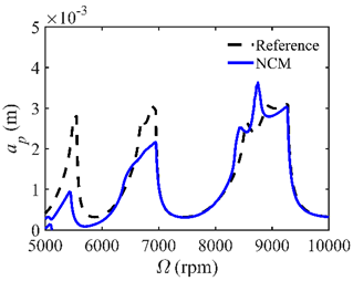
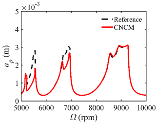
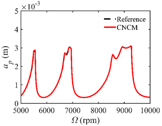
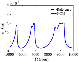
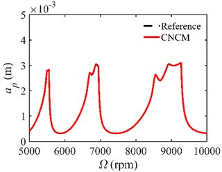
The stability lobe diagrams are given in Table 2 to compare the prediction accuracies of the NCM and CNCM proposed in this paper. The time intervals of the NCM and CNCM proposed in this paper are set to 26, 40, and 56. The reference stability boundaries denoted by the black dashed line are calculated by the SDM with n = 500. The stability lobe diagrams are constructed over a 200 × 100 grid, and the machining parameters are set as follows: Ω [5000 rpm, 10,000 rpm] and ap [0 mm, 5 mm]. It can be seen that the prediction accuracy of the stability lobe diagrams calculated by the CNCM proposed in this paper is higher than that calculated by the NCM.
To further verify the prediction accuracy, the arithmetic mean of the relative error (AMRE) and the mean squared error (MSE) [33] are introduced. They are defined as
A M R E = 1 n e i = 1 n e a i a i 0 a i 0 ,
M S E = 1 n e i = 1 n e a i a i 0 2 ,
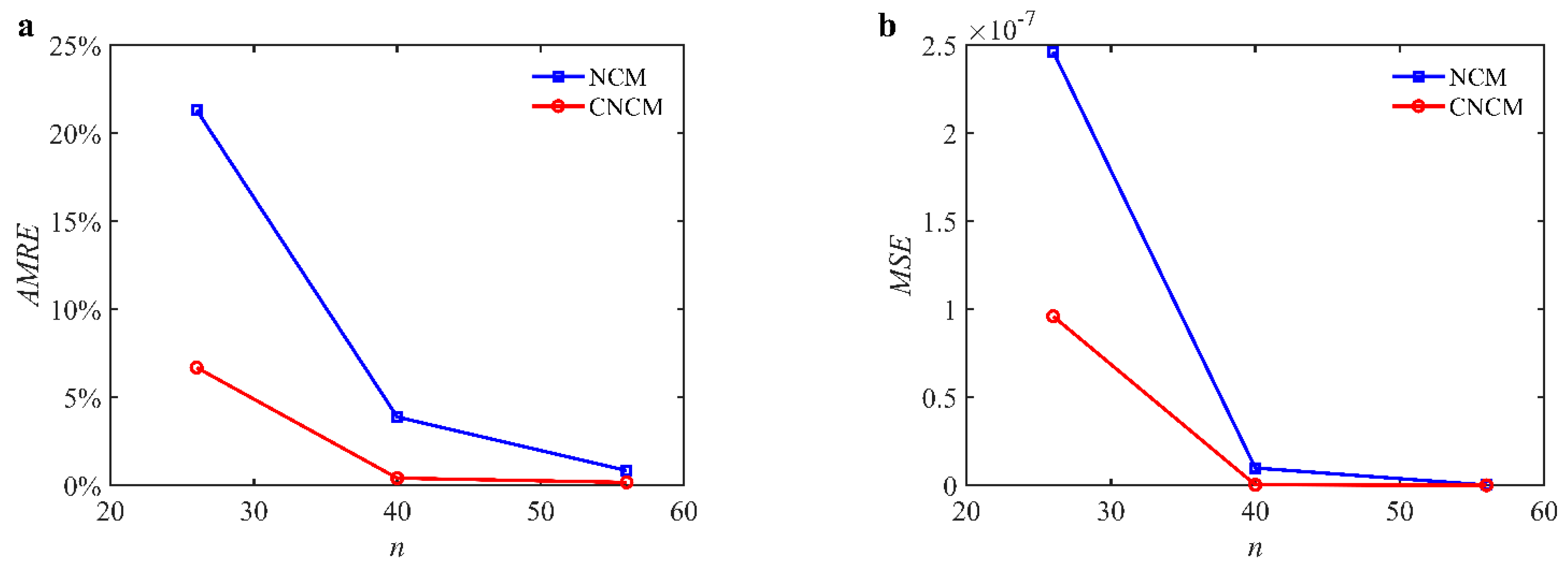
where ai and ai0 denote the predicted and reference axial cutting depths, respectively, and ne denotes the number of discrete points. The AMREs and MSEs are depicted in Figure 2. The AMRE results are given below: When the time interval is 26, the AMREs of the NCM and CNCM proposed in this paper are 21.31% and 6.69%, respectively. When the time interval is 40, the AMREs of the NCM and CNCM proposed in this paper are 3.88% and 0.41%, respectively. When the time interval is 56, the AMREs of the NCM and CNCM proposed in this paper are 0.84% and 0.41%, respectively. The MSE results are given below: When the time interval is 26, the MSEs of the NCM and CNCM proposed in this paper are 2.46 × 10⁻⁷ and 9.60 × 10⁻⁸, respectively. When the time interval is 40, the MSEs of the NCM and CNCM proposed in this paper are 9.85 × 10⁻⁹ and 2.86 × 10⁻¹⁰, respectively. When the time interval is 56, the MSEs of the NCM and CNCM proposed in this paper are 1.73 × 10⁻¹⁰ and 5.28 × 10⁻¹¹, respectively. The results above demonstrate that the proposed CNCM can achieve higher prediction accuracy than the NCM.

4.3. Computational Efficiency

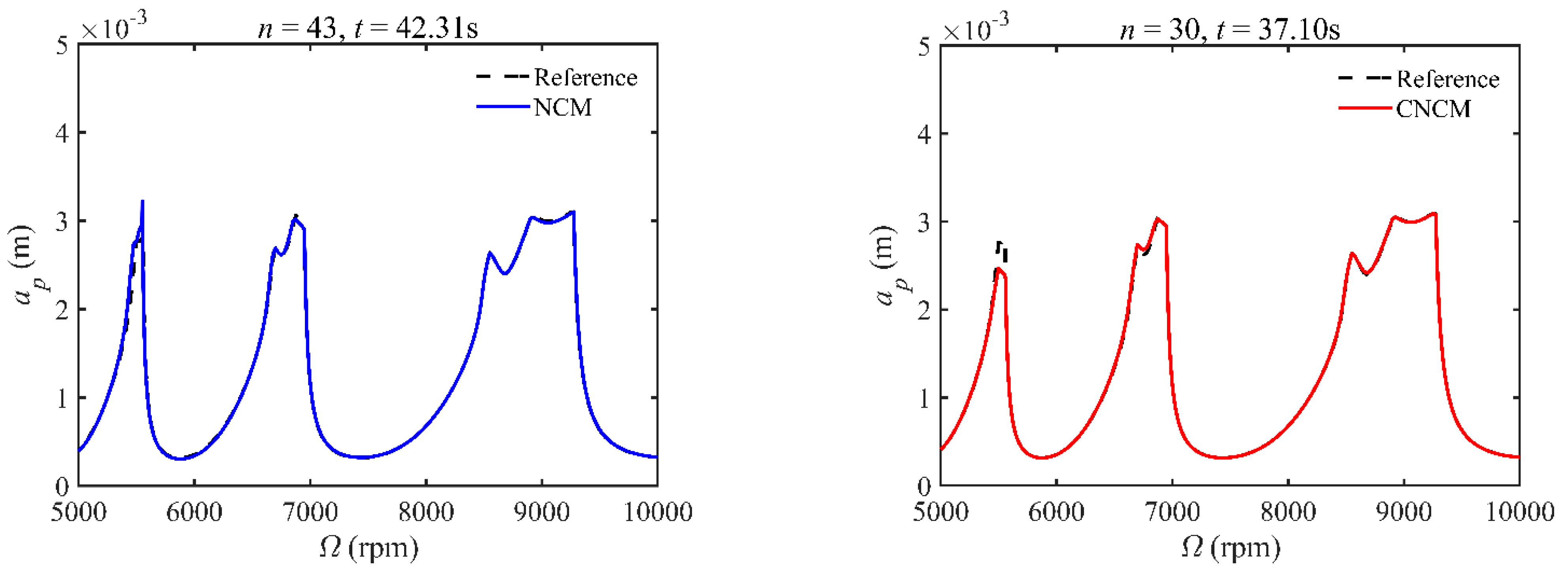
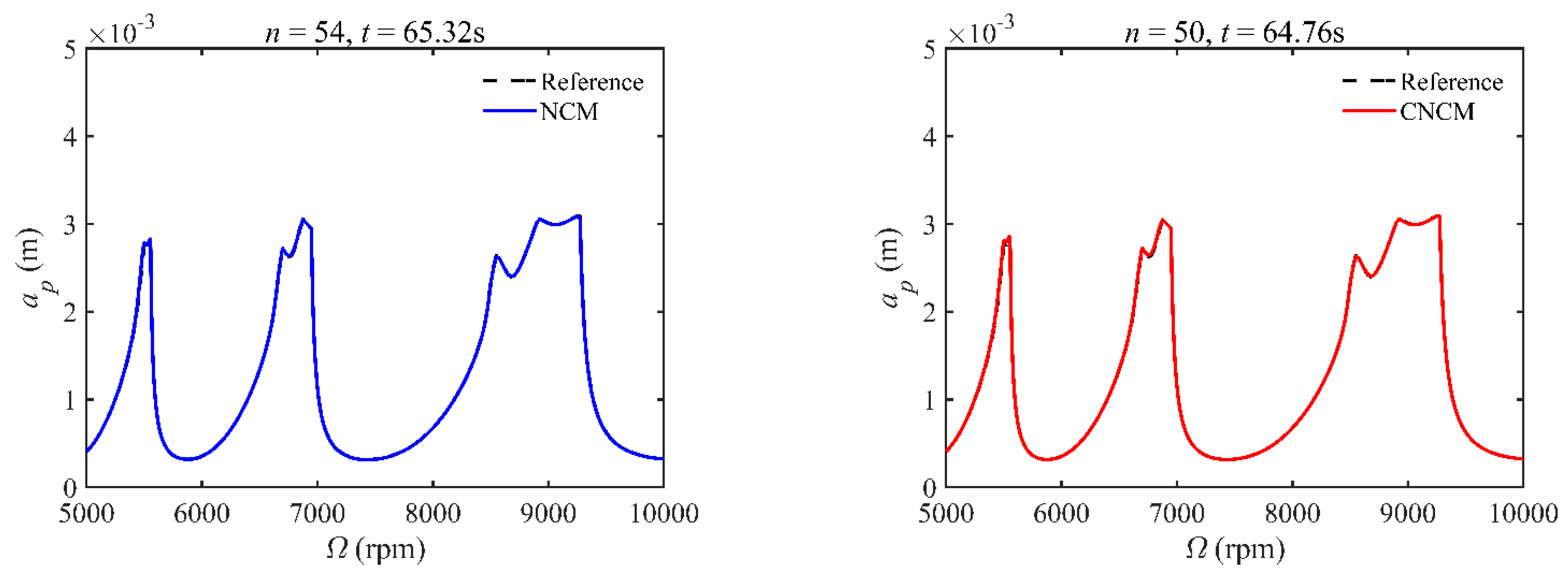
A stability analysis method with a high convergence rate typically requires more computation time [34]. To verify that the proposed method has a relatively ideal computation efficiency, the computational times of the NCM and CNCM at the same AMRE and MSE are discussed. As shown in Figure 3, when AMRE = 1.75%, n = 43 and t = 43.31 s are determined by the NCM, whereas n = 30 and t = 37.10 s are determined by the CNCM proposed in this paper. It is noted that the computational time can be significantly reduced with the CNCM proposed in this paper. It can also be seen that, although the two discrete numbers are different, the prediction stability boundary obtained with the CNCM proposed in this paper is below the reference stability boundary when Ω [5000 rpm, 6000 rpm]. To avoid chatter, the machining parameters selected according to the above-mentioned prediction stability boundary are more reliable. In addition, when MSE = 1.12 × 10⁻¹⁰, the discrete numbers and the computational time, as well as the prediction stability boundaries, are shown in Figure 4. The discrete number obtained with the NCM is greater than that obtained with the CNCM proposed in this paper. However, the computational efficiency of the NCM is slightly lower than that of the CNCM proposed in this paper.

5. Experimental Verification

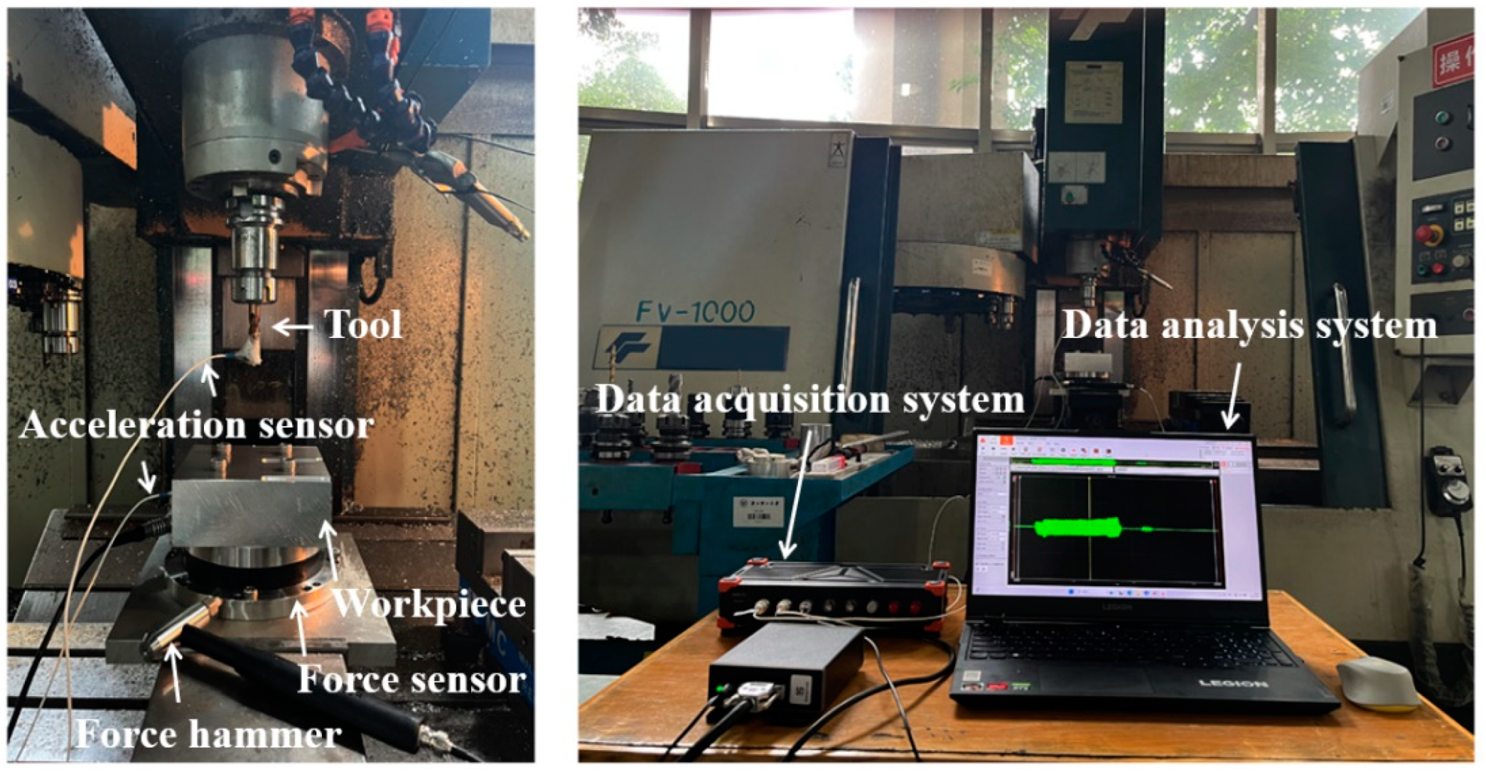
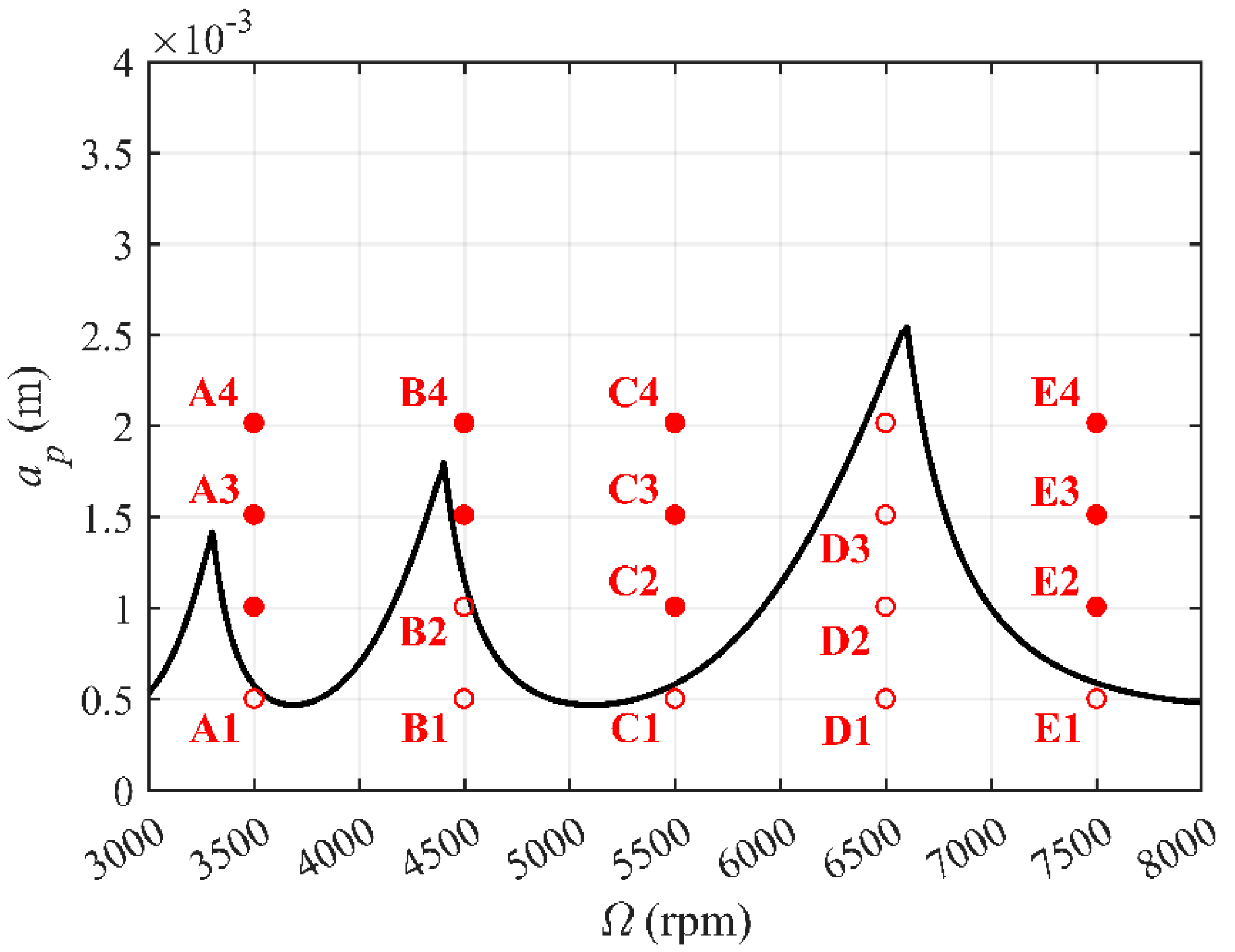
To further verify the effectiveness and superiority of the proposed CNCM, milling experiments were carried out with a feed per tooth of 0.06 mm, Ω [3000 rpm, 8000 rpm] and ap [0 mm, 4 mm]. The milling system was a benchmark system with two DOFs. The workpiece material was aluminum 7075. Before milling experiments, the frequency response function (FRF) of tool should be obtained first. Thus, the hammer experiment is carried out. The measuring instruments include the Kistler 9724A5000 force hammer, Endvco 2256B-10 acceleration sensor, ATI omega-160 force sensor, DEWEsoft SIRIUSI-8xACC data acquisition system and DEWEsoft data analysis system, as shown in Figure 5. The physical and machining parameters of the Harmer experiment are listed in Table 3. A stability lobe diagram of the proposed CNCM is depicted in Figure 6. It can be noted that 20 points are selected from the stability lobe diagram as the test points.
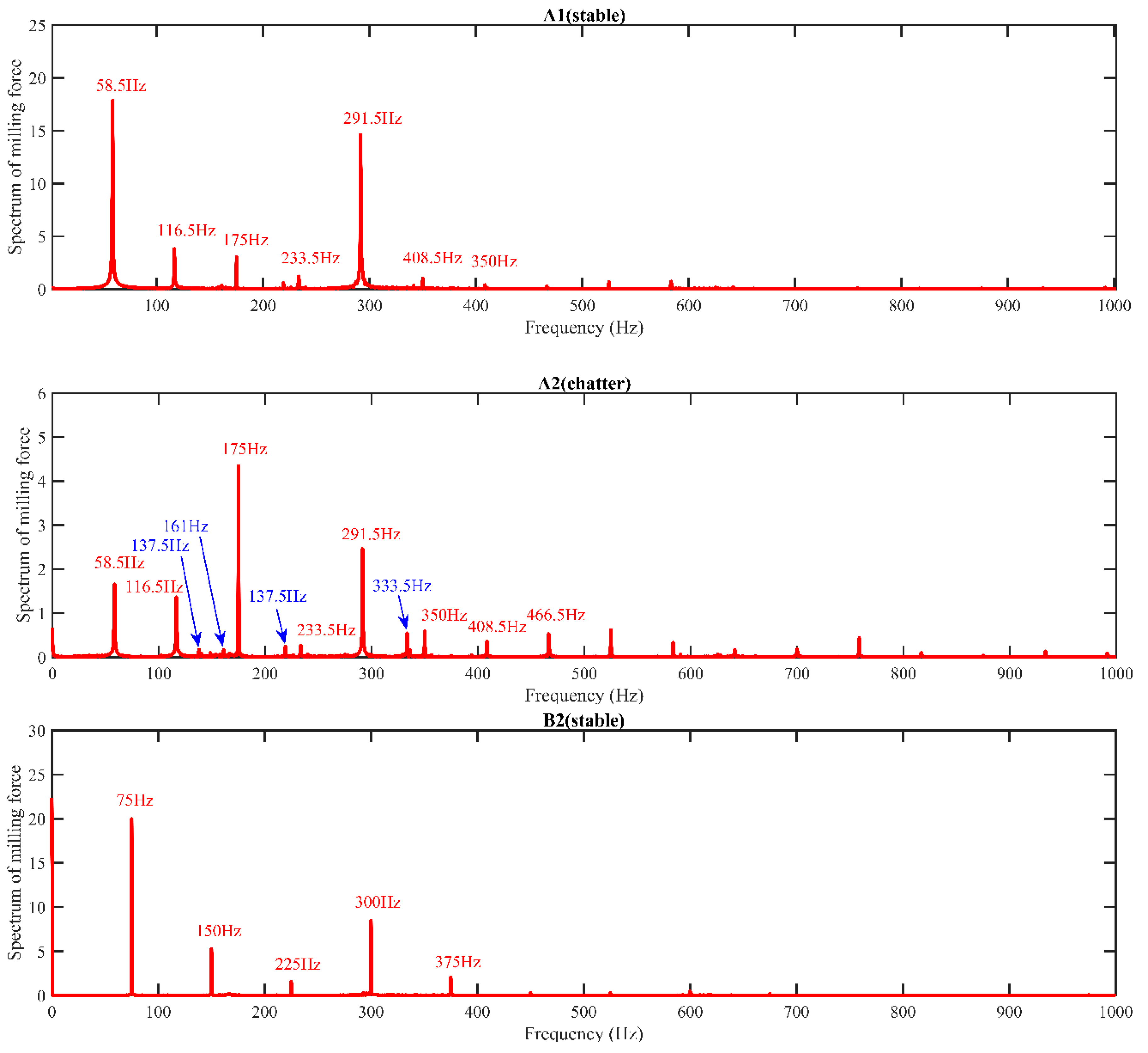
The amplitude spectrum of the milling force signal can show many details in the frequency domain, which can be used to verify the prediction accuracy of the SLD presented in Figure 6. Ten critical points are selected as the milling parameters, and the milling force is measured by an ATI force sensor with a sample rate of 8000. When the milling process is stable, there is only one tooth passing frequency in the spectrum. However, when chatter occurs, there will be a series of disorders in the frequency spectrum. As shown in Figure 7, the milling system has the tooth passing frequency and its harmonic frequency (red value) during stable cutting situations corresponding to A1 (3500 rpm, 0.5 mm), B2 (4500 rpm, 1 mm), C1 (5500 rpm, 0.5 mm), D3 (6500 rpm, 1.5 mm), D4 (6500 rpm, 2 mm), and E1 (7500 rpm, 0.5 mm). It also has chatter frequency (blue value) during unstable cutting situations, corresponding to A2 (3500 rpm, 1 mm), B3 (4500 rpm, 1.5 mm), C2 (5500 rpm, 1 mm), and E2 (7500 rpm, 1 mm). It can be concluded that select milling parameters above the boundary will chatter, while those below the boundary can stabilize the milling process.
Take A1–A4 as examples. A1: Ω = 3500 rpm and ap = 0.5 mm. A2: Ω = 3500 rpm and ap = 1 mm. A3: Ω = 3500 rpm and ap = 1.5 mm. A4: Ω = 3500 rpm and ap = 2 mm. The machined surfaces corresponding to A1–A4 are shown in Figure 8. When chatter occurs, the quality of the machined surface is poor. It can be seen that the chatter becomes increasingly obvious as the depth of the cut increases. The machined surface roughness values are listed in Table 4. Under the conditions of A1–A4, the average values of the machined surface roughness are 1.358, 2.392, 2.462, and 2.910 μm, respectively. It is obvious that the chatter significantly decreases the machined surface quality. The machined surface roughness under the conditions of B1–B4, C1–C4, D1–D4, and E1–E4 is also listed in Table 4. It can be observed that, under the conditions of A1, B1, B2, C1, D1–D4, and E1, the average values of the machined surface roughness are 1.358, 1.181, 1.501, 1.363, 1.312, 1.514, 1.655, 1.937, and 1.305 μm, respectively. The results show that the cutting parameters below the stability boundary can avoid chatter as much as possible, thereby ensuring the quality of the machined surface.

6. Conclusions

This study focuses on the convergence rate and prediction accuracy of the milling stability based on the composited Newton–Cotes formula. For example, when the discrete number is 40, the convergence rate and prediction accuracy improve about 4.1 and 9.4 times, respectively, while computational efficiency is similar. The reason is that because the proposed method considers three intermediate interpolation points, the local discrete error of the proposed method is smaller than that of the comparison method, which ensures the prediction accuracy of the proposed method. The state transition matrix of the proposed method is divided into three submatrices, which can avoid double calculation and matrix multiplication. The simulation results of the milling model with a single DOF validate that the proposed method has a high convergence rate and prediction accuracy while ensuring computational efficiency. The experimental results of the milling model with two DOFs validate that the machining parameters below the prediction stability boundary obtained with the proposed method can avoid chatter as much as possible while ensuring the machined surface quality.

Author Contributions

Conceptualization, J.Z. and X.D.; methodology, J.Z.; software, P.R.; validation, C.Z.; formal analysis, P.R.; investigation, P.R.; resources, J.Z.; data curation, C.Z.; writing—original draft preparation, P.R.; writing—review and editing, X.D.; visualization, P.R.; supervision, X.D.; project administration, X.D.; funding acquisition, J.Z. and X.D. All authors have read and agreed to the published version of the manuscript.

Funding

This research was funded by [Natural Science Foundation of Zhejiang Province] grant number [LY21E050022], [National Natural Science Foundation of China] grant number [52005142] and number [52275469], and [Postdoctoral research activities of Anhui Province] postdoctoral number [934704]. And The APC was funded by [52275469]. The authors would like to thank the School of Mechanical Engineering, Hefei University of Technology, and the School of Mechanical Engineering, Zhejiang Sci-Tech University.

Data Availability Statement

The data presented in this study are available on request from the corresponding author.

Conflicts of Interest

The authors declare no conflict of interest.

References

  1. Ma, J.; Li, Y.; Zhang, D.; Zhao, B.; Wang, G.; Pang, X. A Novel Updated Full-Discretization Method for Prediction of Milling Stability. Micromachines 2022, 13, 160. [Google Scholar] [CrossRef]
  2. Yan, Y.; Xu, J.; Wiercigroch, M. Modelling of regenerative and frictional cutting dynamics. Int. J. Mech. Sci. 2019, 156, 86–93. [Google Scholar] [CrossRef]
  3. Yue, C.; Gao, H.; Liu, X.; Liang, S.Y.; Wang, L. A review of chatter vibration research in milling. Chin. J. Aeronaut. 2019, 32, 215–242. [Google Scholar] [CrossRef]
  4. Quintana, G.; Ciurana, J. Chatter in machining processes: A review. Int. J. Mach. Tools Manfacture 2011, 51, 363–376. [Google Scholar] [CrossRef]
  5. Rafal, R.; Pawel, L.; Krzysztof, K.; Bogdan, K. Chatter identification methods on the basis of time series measured during titanium superalloy milling. Int. J. Mech. Sci. 2015, 99, 196–207. [Google Scholar] [CrossRef]
  6. Albertelli, P.; Braghieri, L.; Torta, M.; Monno, M. Development of a generalized chatter detection methodogy for variable speed machining. Mech. Syst. Signal Process. 2019, 123, 26–42. [Google Scholar] [CrossRef]
  7. Ji, Y.; Wang, X.; Liu, Z.; Wang, H.; Jiao, L.; Wang, D.; Leng, S. Early milling chatter identification by improved empirical mode decomposition and multi-indicator synthetic evaluation. J. Sound Vib. 2018, 433, 138–159. [Google Scholar] [CrossRef]
  8. Munoa, J.; Beudaert, X.; Dombovari, Z.; Altintas, Y.; Budak, E.; Brecher, C.; Stepan, G. Chatter suppression techniques in metal cutting. CIRP Ann. 2016, 65, 785–808. [Google Scholar] [CrossRef]
  9. Shi, J.; Song, Q.; Liu, Z.; Wan, Y. Formulating a numerically low-cost method of a constrained layer damper for vibration suppression in thin-walled component milling and experimental validation. Int. J. Mech. Sci. 2017, 128–129, 294–311. [Google Scholar] [CrossRef]
  10. Zhang, Z.; Li, H.; Liu, X.; Zhang, W.; Meng, G. Chatter mitigation for the milling of thin-walled workpiece. Int. J. Mech. Sci. 2018, 138–139, 262–271. [Google Scholar] [CrossRef]
  11. Song, Q.; Liu, Z.; Wan, Y.; Ju, G.; Shi, J. Application of Sherman-Morrison-Woodbury formulas in instantaneous dynamic of peripheral milling for thin-walled component. Int. J. Mech. Sci. 2015, 96–97, 79–90. [Google Scholar] [CrossRef]
  12. Altintas, Y.; Weck, M. Chatter stability of metal cutting and grinding. CIRP Ann. 2004, 53, 619–642. [Google Scholar] [CrossRef]
  13. Wiercigtoch, M.; Budak, E. Sources of nonlinearities, chatter generation and suppression in metal cutting. Philos. Trans. R. Soc. A Math. Phys. Eng. Sci. 2001, 359, 663–693. [Google Scholar] [CrossRef] [Green Version]
  14. Altintas, Y.; Budak, E. Analytical prediction of stability lobes in milling. CIRP Ann. 1995, 44, 357–362. [Google Scholar] [CrossRef]
  15. Merdol, S.D.; Altintas, Y. Multi frequency solution of chatter stability for low immersion milling. J. Manuf. Sci. Eng. 2004, 126, 459. [Google Scholar] [CrossRef]
  16. Insperger, T.; Stepan, G. Semi-discretization method for delayed systems. Int. J. Numer. Methods Eng. 2002, 55, 503–518. [Google Scholar] [CrossRef]
  17. Insperger, T.; Stepan, G. Updated semi-discretization method for periodic delay-differential equations with discrete delay. Int. J. Numer. Methods Eng. 2004, 61, 117–141. [Google Scholar] [CrossRef]
  18. Jiang, S.; Sun, Y.; Yuan, X.; Liu, W. A second-order semi-discretization method for the efficient and accurate stability prediction of milling process. Int. J. Adv. Manuf. Technol. 2017, 92, 583–595. [Google Scholar] [CrossRef]
  19. Ding, Y.; Zhu, L.; Zhang, X.; Ding, H. A full-discretization method for prediction of milling stability. Int. J. Mach. Tools Manuf. 2010, 50, 502–509. [Google Scholar] [CrossRef]
  20. Ding, Y.; Zhu, L.; Zhang, X.; Ding, H. Second-order full discretization method for milling stability prediction. Int. J. Mach. Tools Manuf. 2010, 50, 926–932. [Google Scholar] [CrossRef]
  21. Yan, Z.; Wang, X.; Liu, Z.; Wang, D.; Li, J.; Ji, Y. Third-order updated full-discretization method for milling stability prediction. Int. J. Adv. Manuf. Technol. 2017, 92, 2299–2309. [Google Scholar] [CrossRef]
  22. Ding, Y.; Zhu, L.; Zhang, X.; Ding, H. Numerical integration method for prediction of milling stability. J. Manuf. Sci. Eng. 2011, 133, 031005. [Google Scholar] [CrossRef]
  23. Dong, X.; Qiu, Z. Stability analysis in milling process based on updated numerical integration method. Mech. Sytems Signal Process. 2020, 137, 106435. [Google Scholar] [CrossRef]
  24. Li, W.; Wang, L.; Yu, G. An accurate and fast milling stability prediction approach based on the Newton-Cotes rules. Int. J. Mech. Sci. 2020, 177, 105469. [Google Scholar] [CrossRef]
  25. Qin, C.; Tao, J.; Li, L. An Adams-Moulton-based method for stability prediction of milling processes. Int. J. Adv. Manuf. Technol. 2017, 89, 3049–3058. [Google Scholar] [CrossRef]
  26. Lehotzky, D.; Insperger, T.; Khasawneh, F.; Stepan, G. Spectral element method for stability analysis of milling processes with discontinuous time-periodicity. Int. J. Adv. Manuf. Technol. 2017, 89, 2503–2514. [Google Scholar] [CrossRef] [Green Version]
  27. Ramirez, L.F.; Saldivar, B.; Vilchis, J.C.A.; Oca, S.M. Lyapunov-Krasovskii approach to the stability analysis of the milling process. IET Control Theory Appl. 2018, 12, 1332–1339. [Google Scholar] [CrossRef]
  28. Simos, T.E. Closed Newton—Cotes trigonometrically-fitted formulae of high order for long-time integration of orbital problems. Appl. Math. Lett. 2009, 22, 1616–1621. [Google Scholar] [CrossRef]
  29. Burg, C.O.E. Derivative-based closed Newton–Cotes numerical quadrature. Appl. Math. Comput. 2012, 218, 7052–7065. [Google Scholar] [CrossRef]
  30. Odibat, Z.M. Differential transform method for solving Volterra integral equation with separable kernels. Math. Comput. Model. 2008, 48, 1144–1149. [Google Scholar] [CrossRef]
  31. Qin, C.; Tao, J.; Shi, H.; Xiao, D.; Li, B.; Liu, C. A novel Chebyshev-wavelet-based approach for accurate and fast prediction of milling stability. Precis. Eng. 2020, 62, 244–255. [Google Scholar] [CrossRef]
  32. Hajdu, D.; Borgioli, F.; Michiels, W.; Insperger, T.; Stepan, G. Robust stability of milling operations based on pseudospectral approach. Int. J. Mach. Tools Manuf. 2020, 149, 103516. [Google Scholar] [CrossRef]
  33. Yan, Z.; Zhang, C.; Jia, J.; Ma, B.; Jiang, X.; Wang, D.; Zhu, T. High-order semi-discretization methods for stability analysis in milling based on precise integration. Precis. Eng. 2022, 73, 71–92. [Google Scholar] [CrossRef]
  34. Lou, W.; Qin, G.; Zuo, D. Investigation on Cotes-formula-based prediction method and its experimental verification of milling stability. J. Manuf. Process. 2021, 64, 1077–1088. [Google Scholar] [CrossRef]
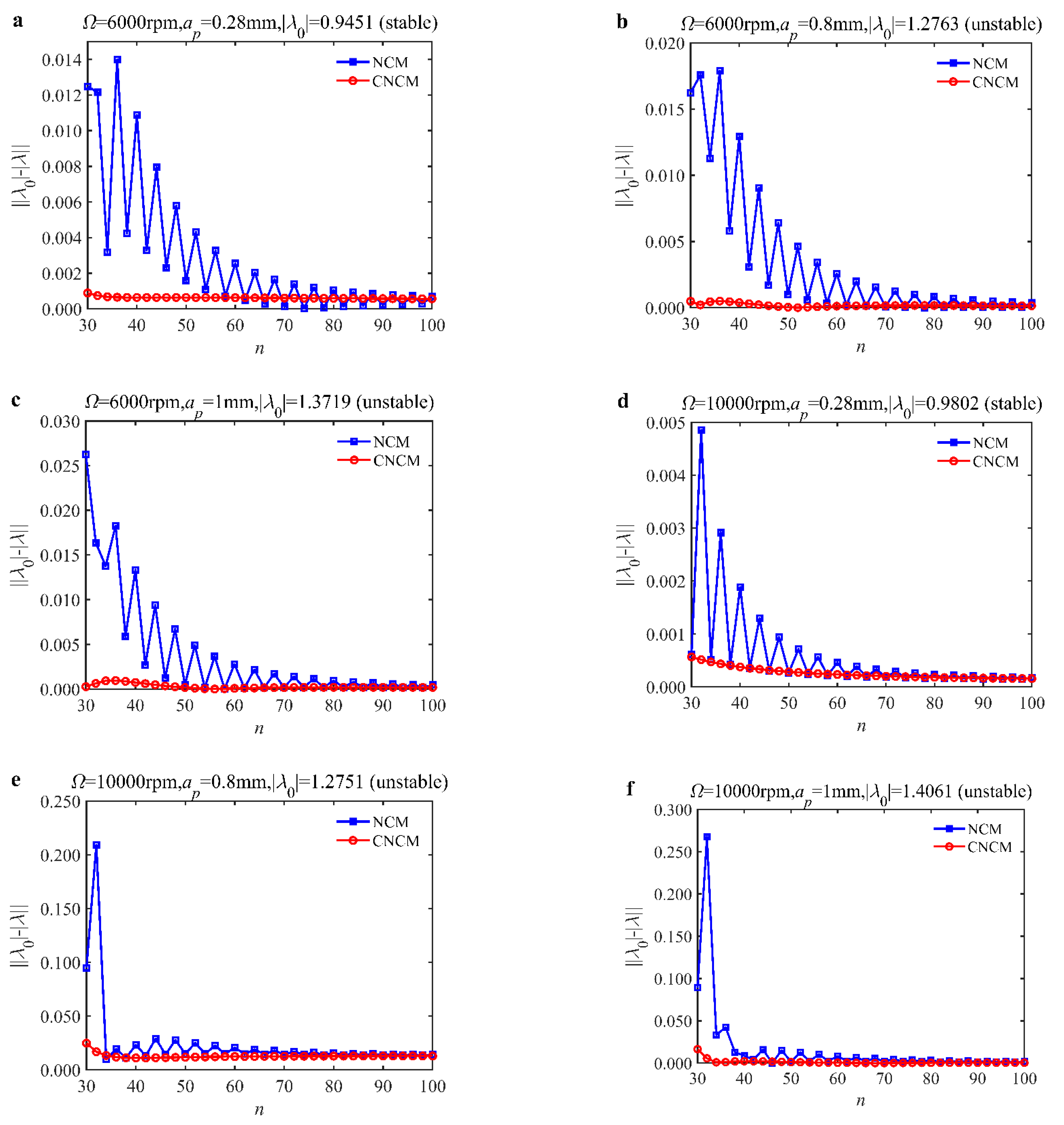
Figure 1. Convergence rate comparisons between the NCM and the CNCM proposed in this paper. (a) Ω = 6000 rpm, ap = 0.28 mm, and λ 0 = 0.9451 (stable); (b) Ω = 6000 rpm, ap = 0.8 mm, and λ 0 = 1.2763 (unstable); (c) Ω = 6000 rpm, ap = 1 mm, and λ 0 = 1.3719 (unstable); (d) Ω = 10,000 rpm, ap = 0.28 mm, and λ 0 = 0.9802 (stable); (e) Ω = 10,000 rpm, ap = 0.8 mm, and λ 0 = 1.2751 (unstable); (f) Ω = 10,000 rpm, ap = 1 mm, and λ 0 = 1.4061 (unstable).
Micromachines 14 01304 g001
Figure 2. AMRE and MSE comparisons between the NCM and the CNCM proposed in this paper. (a) AMRE comparisons when n = 26, n = 40 and n = 56; (b) MSE comparisons when n = 26, n = 40 and n = 56.
Micromachines 14 01304 g002
Figure 3. Computational time comparisons between the NCM and the CNCM proposed in this paper when AMRE = 1.75%.
Micromachines 14 01304 g003
Figure 4. Computational time comparisons between the NCM and the CNCM proposed in this paper when MSE = 1.12 × 10⁻¹⁰.
Micromachines 14 01304 g004
Figure 5. Experiments platform, measuring instruments and calibration process.
Micromachines 14 01304 g005
Figure 6. Predicted stability lobe diagram with the CNCM proposed in this paper, where hollow and filled circles denote stable and unstable cutting situations, respectively. A1: Ω = 3500 rpm, ap = 0.5 mm; A2: Ω = 3500 rpm, ap = 1 mm; A3: Ω = 3500 rpm, ap = 1.5 mm; A4: Ω = 3500 rpm, ap = 2 mm. B1: Ω = 4500 rpm, ap = 0.5 mm; B2: Ω = 4500 rpm, ap = 1 mm; B3: Ω = 4500 rpm, ap = 1.5 mm; B4: Ω = 4500 rpm, ap = 2 mm. C1: Ω = 5500 rpm, ap = 0.5 mm; C2: Ω = 5500 rpm, ap = 1 mm; C3: Ω = 5500 rpm, ap = 1.5 mm; C4: Ω = 5500 rpm, ap = 2 mm. D1: Ω = 6500 rpm, ap = 0.5 mm; D2: Ω = 6500 rpm, ap = 1 mm; D3: Ω = 6500 rpm, ap = 1.5 mm; D4: Ω = 6500 rpm, ap = 2 mm. E1: Ω = 7500 rpm, ap = 0.5 mm; E2: Ω = 7500 rpm, ap = 1 mm; E3: Ω = 7500 rpm, ap = 1.5 mm; E4: Ω = 7500 rpm, ap = 2 mm.
Micromachines 14 01304 g006
Figure 7. The amplitude spectrum of measured points.
Micromachines 14 01304 g007aMicromachines 14 01304 g007bMicromachines 14 01304 g007c
Figure 8. Machined surface of Aluminium 7075 with the cutting parameters corresponding to A1–A4, where 1, 2, and 3 in white denote three different sampling points.
Micromachines 14 01304 g008
Table 1. Physical and machining parameters of the benchmark example with a single DOF [24].
ParametersSymbolsValues
Modal mass (kg)mt0.03993
Damping ratioζ0.011
Natural frequency (Hz)ωn922 × 2π
Tangential linearized cutting force coefficient (N/m)Kt6 × 108
Normal linearized cutting force coefficient (N/m)Kn2 × 108
Number of tool teethNt2
Radial immersion ratioa/D1
Table 2. Stability lobe diagrams with the NCM and CNCM proposed in this paper.
nNCMCNCM
26Micromachines 14 01304 i001Micromachines 14 01304 i002
40Micromachines 14 01304 i003Micromachines 14 01304 i004
56Micromachines 14 01304 i005Micromachines 14 01304 i006
Table 3. Physical and machining parameters of the Harmer experiment with two DOFs.
ParametersSymbolsValues
Modal mass (kg)mt0.274
Damping ratioζ0.0338
Natural frequency (Hz)ωn876 × 2π
Tangential linearized cutting force coefficient (N/m)Kt5.5 × 108
Normal linearized cutting force coefficient (N/m)Kn3.75 × 108
Number of tool teethNt4
Tool diameter (m)D0.012
Radio immersion ratioa/D1
Table 4. Machined surface roughness of Aluminium 7075 with the machining parameters corresponding to A1–A4, B1–B4, C1–C4, D1–D4, and E1–E5.
Serial NumbersSurface Roughness of the Measured Points (μm)
123Average Values
A11.4901.6471.7381.625
A22.9972.0532.1272.392
A32.8792.1352.3712.462
A42.9672.8172.9472.910
B11.0681.1901.2861.181
B21.4961.4471.5611.501
B32.2872.3322.3172.312
B42.2422.2942.1432.226
C11.0891.5941.4071.363
C22.3352.4862.3582.393
C32.4232.5062.7122.547
C42.6732.6852.8372.732
D11.2651.3301.3401.312
D21.5631.4531.5261.514
D31.7441.4751.7451.655
D41.9971.9451.8681.937
E11.3741.2691.2731.305
E23.2862.8813.0663.078
E33.2933.7922.7753.287
E43.6093.3603.3793.449
Disclaimer/Publisher’s Note: The statements, opinions and data contained in all publications are solely those of the individual author(s) and contributor(s) and not of MDPI and/or the editor(s). MDPI and/or the editor(s) disclaim responsibility for any injury to people or property resulting from any ideas, methods, instructions or products referred to in the content.