
Tunable Device for Long Focusing in the Sub-THz Frequency Range Based on Fresnel Mirrors

Abstract
:1. Introduction
2. Theory
2.1. Working Principle
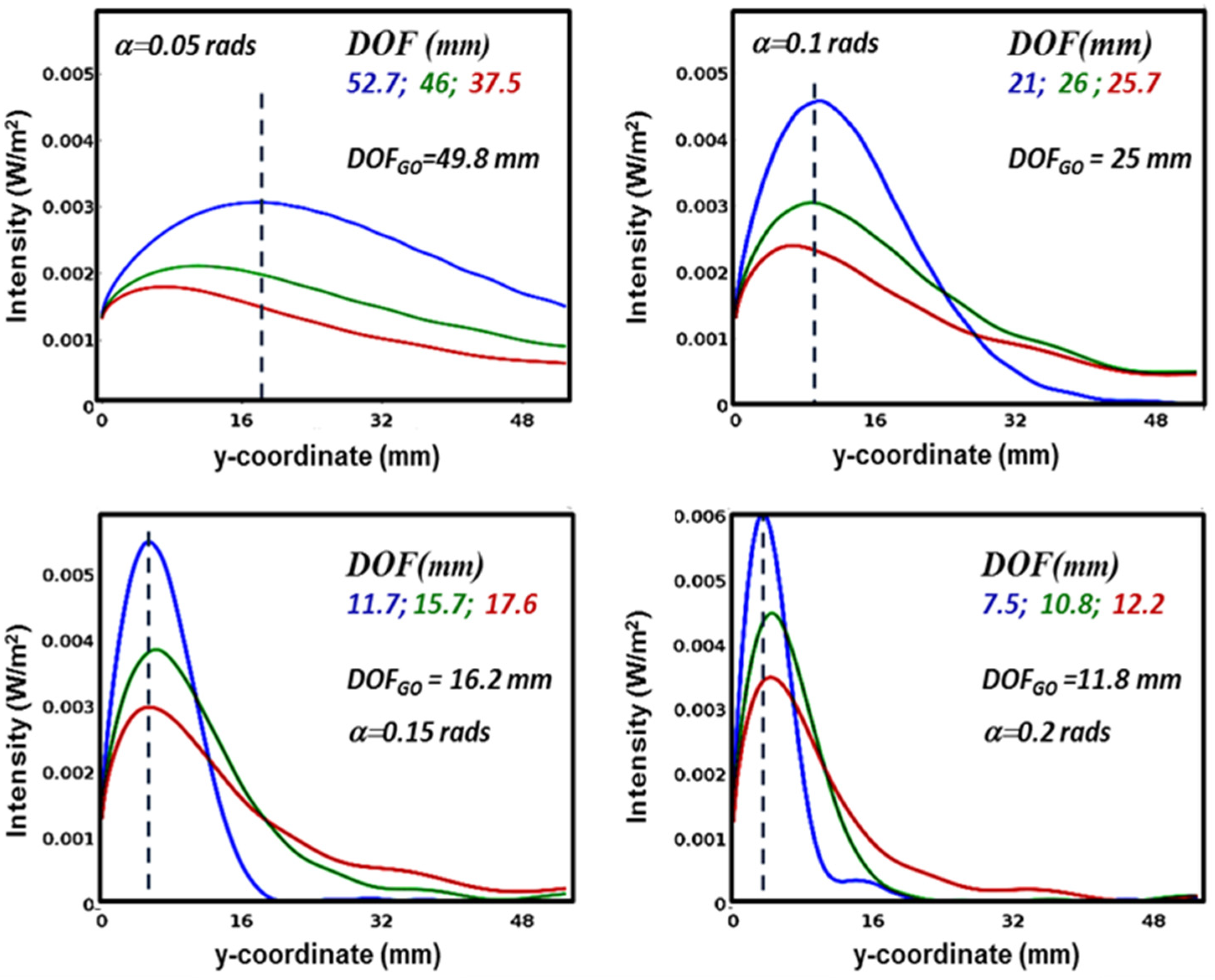
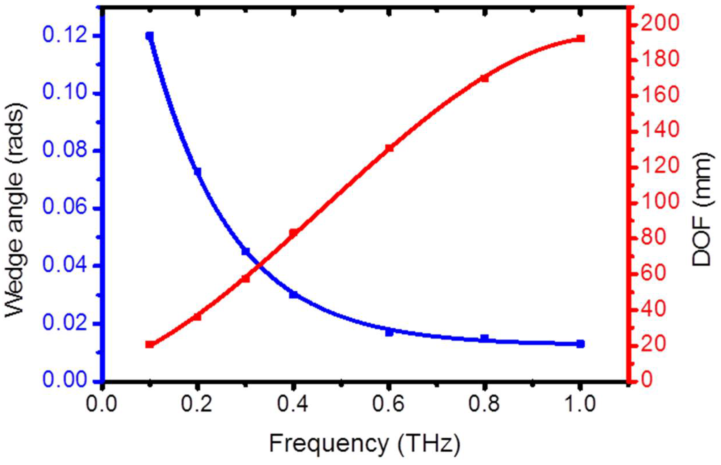
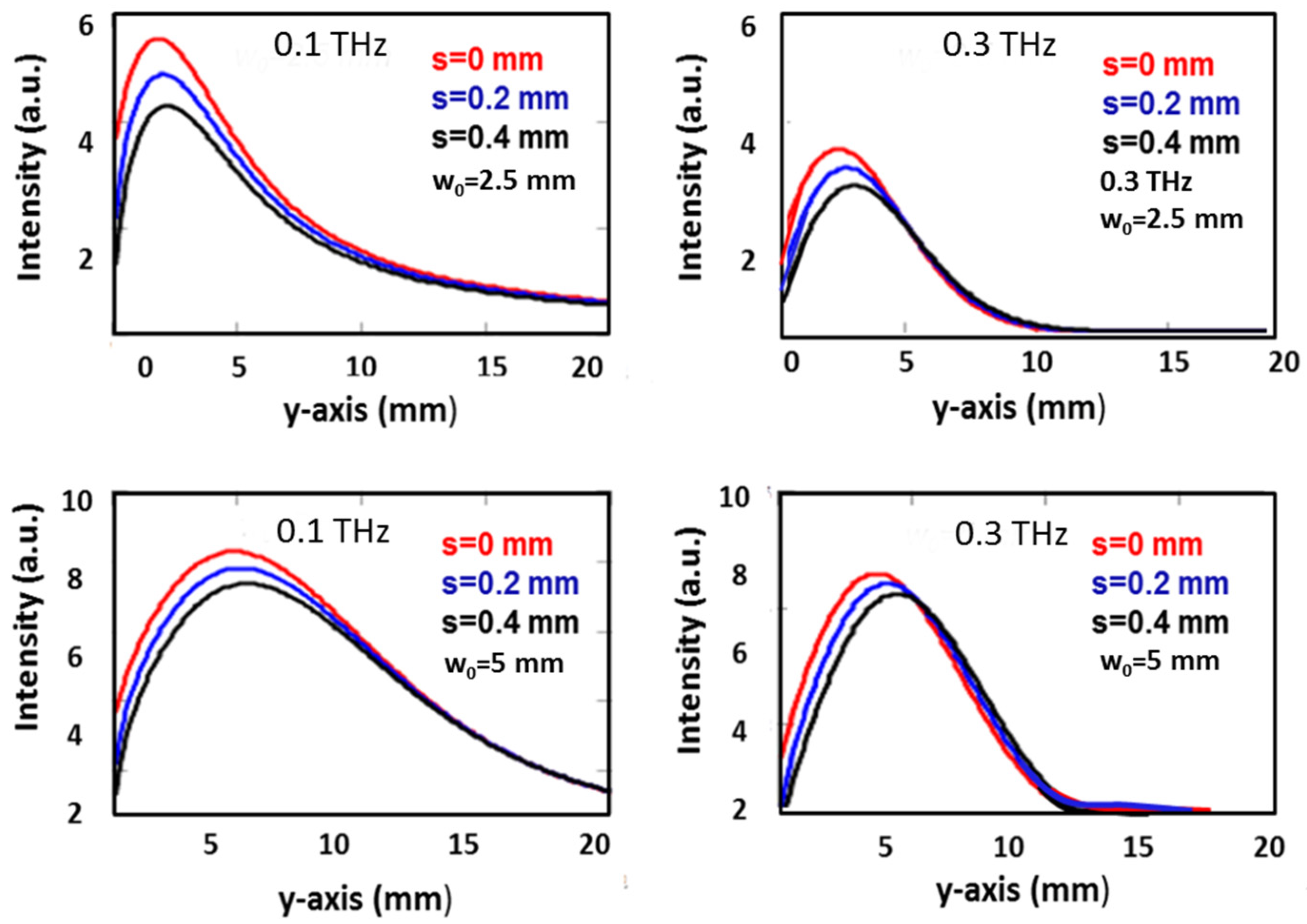
2.2. Simulation Results
3. Experimental Tests
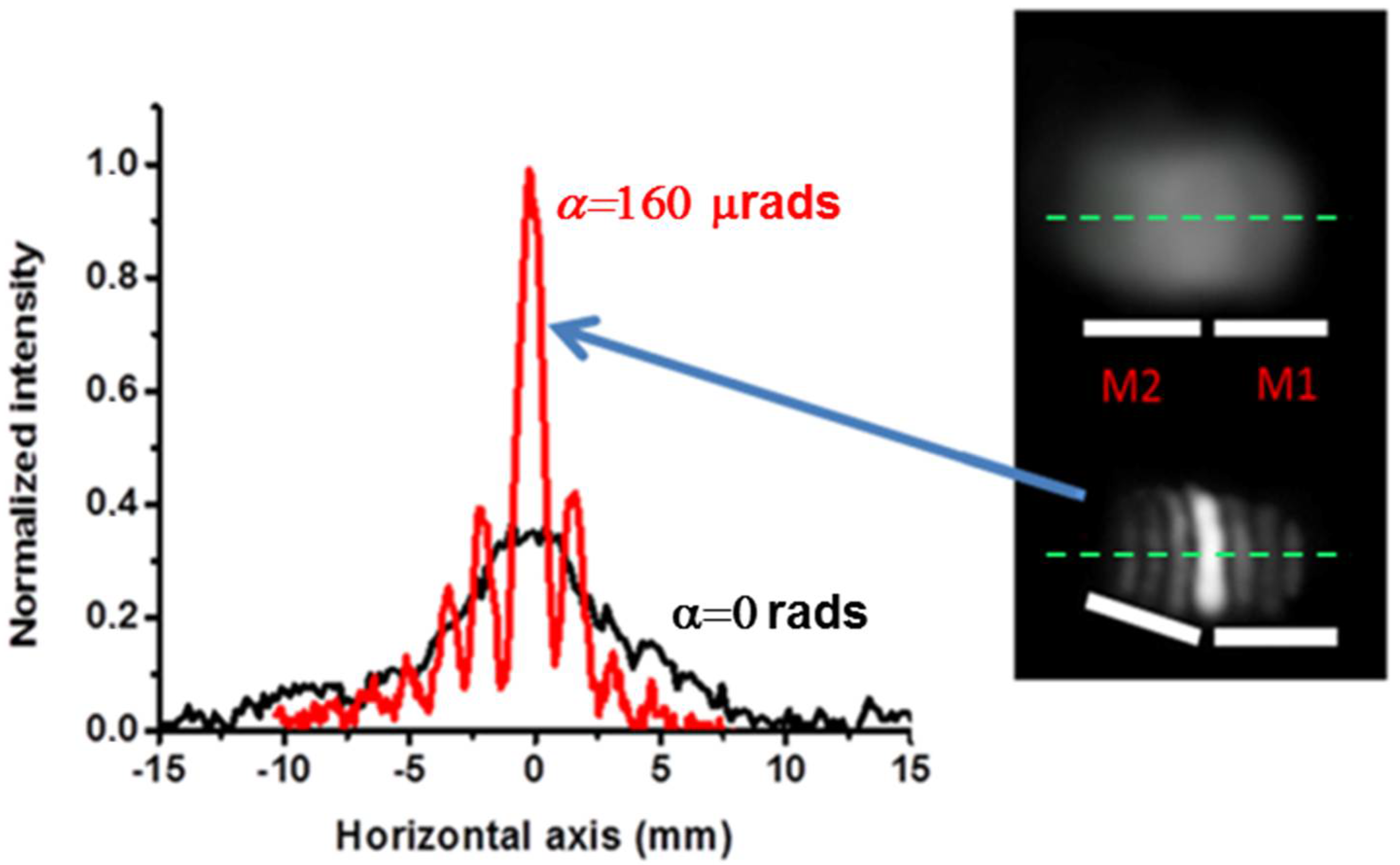
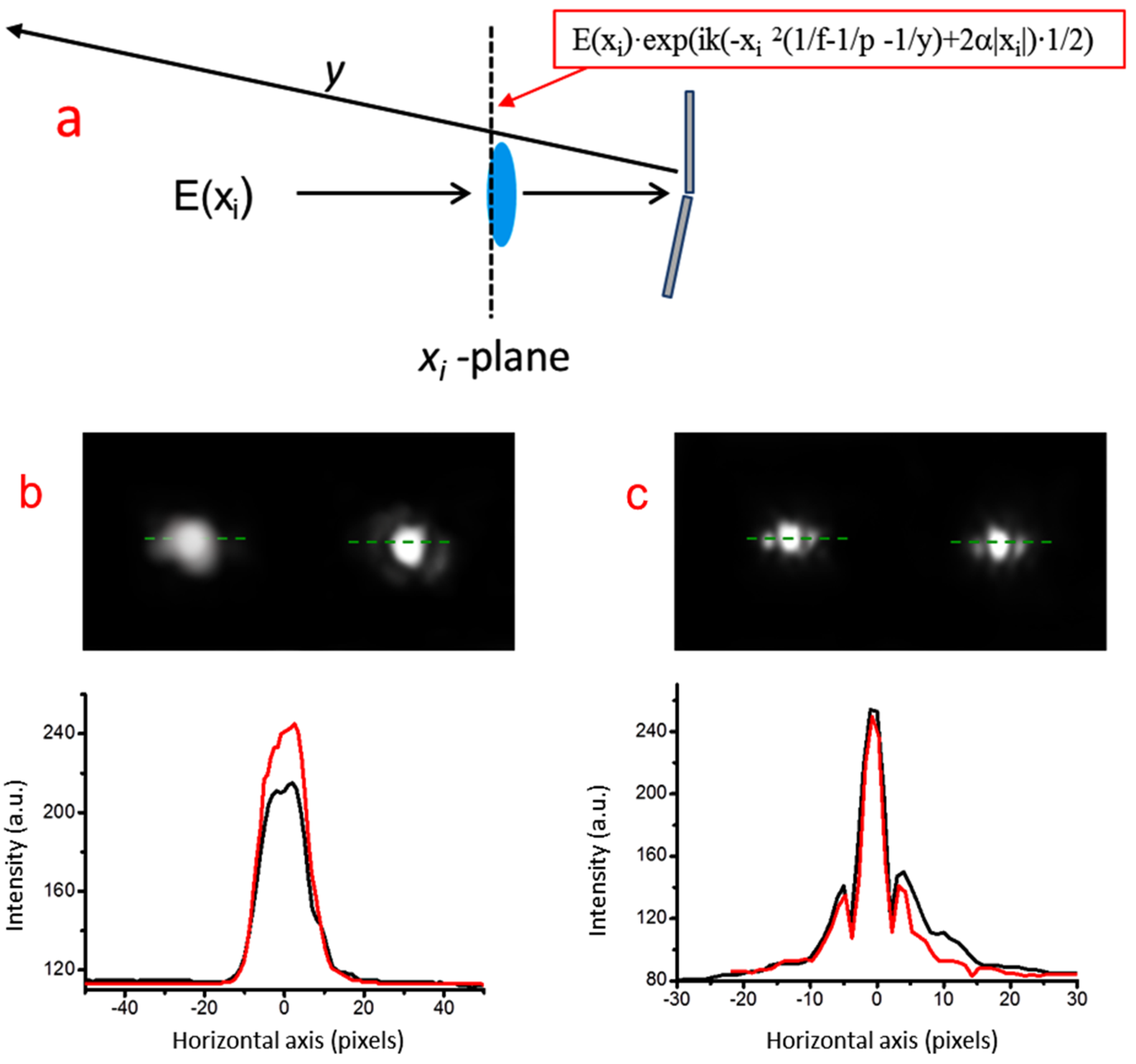
3.1. Principle of the Measurement
3.2. Experimental Results and Discussion
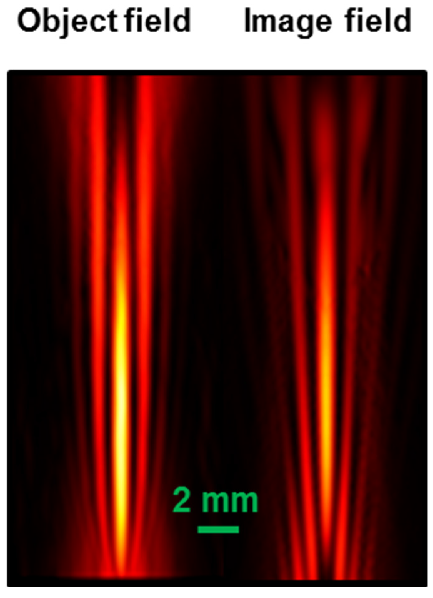
3.3. Preliminary Comparative Tests with THz Radiation
4. Conclusions
Author Contributions
Funding
Data Availability Statement
Conflicts of Interest
References
- Musina, G.; Dolganova, I.; Chernomyrdin, N.; Gavdush, A.; Ulitko, V.; Cherkasova, O.; Tuchina, D.; Nikitin, P.; Alekseeva, A.; Bal, N.; et al. Optimal hyperosmotic agents for tissue immersion optical clearing in terahertz biophotonics. J. Biophotonics 2020, 13, e202000297. [Google Scholar] [CrossRef] [PubMed]
- Hernandez-Serrano, A.; Corzo-Garcia, S.; Garcia-Sanchez, E.; Alfaro, M.; Castro-Camus, E. Quality control of leather by terahertztime-domain spectroscopy. Appl. Opt. 2014, 20, 7872–7876. [Google Scholar] [CrossRef] [PubMed]
- Ma, J.; Karl, N.J.; Bretin, S.; Ducournau, G.; Mittleman, D.M. Frequency-division multiplexer and demultiplexer for terahertz wireless links. Nat. Commun. 2017, 8, 729. [Google Scholar] [CrossRef] [PubMed]
- Cruz, A.; Cunha, W.; Del Rosso, T.; Dmitriev, V.; Costa, K. Spectral Analysis of a SPR Sensor based on Multilayer Graphene in the Far Infrared Range. J. Microw. Optoelectron. Electromagn. Appl. 2023, 22, 184–195. [Google Scholar] [CrossRef]
- Afsah-Hejri, L.; Hajeb, P.; Ara, P.; Ehsani, R.J. A Comprehensive Review on Food Applications of Terahertz Spectroscopy and Imaging. Comprensive Rev. Food Sci. Food Saf. 2019, 18, 1562–1621. [Google Scholar] [CrossRef] [PubMed]
- Shchepetilnikov, A.V.; Gusikhin, P.A.; Muravev, V.M.; Tsydynzhapov, G.E.; Nefyodov, Y.A.; Dremin, A.A. New Ultra-Fast Sub-Terahertz Linear Scanner for Postal Security Screening. Int. J. Infrared Millim. Waves 2020, 41, 655–664. [Google Scholar] [CrossRef]
- Yachmenev, A.; Lavrukhin, D.; Glinskiy, I.; Zenchenko, N.; Goncharov, Y.; Spektor, I.; Khabibullin, R.; Otsuji, T.; Ponomarev, D. Metallic and dielectric metasurfaces in photoconductive terahertz devices: A review. Opt. Eng. 2019, 59, 061608. [Google Scholar] [CrossRef]
- Sun, Q.; Chen, X.; Liu, X.; Stantchev, R.; Pickwell-MacPherson, E. Exploiting total internal reection geometry for terahertz devices and enhanced sample characterization. Adv. Opt. Mater. 2020, 8, 1900535. [Google Scholar] [CrossRef]
- Wei, X.; Liu, C.; Niu, L.; Zhang, Z.; Wang, K.; Yang, Z.; Liu, J. Generation of arbitrary order Bessel beams via 3D printed axicons at the terahertz frequency range. Appl. Opt. 2015, 54, 10641–10649. [Google Scholar] [CrossRef] [PubMed]
- Ulitko, V.E.; Kurlova, V.N.; Masalova, V.M.; Dolganova, I.N.; Chernomyrdin, N.V.; Zaytsev, K.I.; Katyba, G.M. Terahertz axicon fabricated by direct sedimentation of SiO2 colloidal nanoparticles in a mold. In Proceedings of the Terahertz Emitters, Receivers, and Applications XII, San Diego, CA, USA, 1 August 2021; p. 118270M. [Google Scholar]
- Xiang, F.; Liu, D.; Xiao, L.; Shen, S.; Yang, Z.; Liu, J.; Wang, K. Generation of a meter-scale THz diffraction-free beam based on multiple cascaded lens-axicon doublets: Detailed analysis and experimental demonstration. Opt. Express 2020, 28, 36873–36883. [Google Scholar] [CrossRef] [PubMed]
- Reddy, V.A.K.; Bodet, D.; Arjun, S.; Petrov, V.; Liberale, C.; Jornet, J.M. Ultrabroadband terahertz-band communications with self-healing bessel beams. Comm. Eng. 2023, 2, 70. [Google Scholar] [CrossRef]
- Hernandez-Serrano, A.I.; Pickwell-MacPherson, E. Low cost and long-focal-depth metallic axicon for terahertz frequencies based on parallel-plate-waveguides. Sci. Rep. 2021, 11, 3005. [Google Scholar] [CrossRef] [PubMed]
- Margheri, G.; Del Rosso, T. Long-Focusing Device for Broadband THz Applications Based on a Tunable Reflective Biprism. Micromachines 2023, 14, 1939. [Google Scholar] [CrossRef] [PubMed]
- Makhlouf, S.; Cojocari, O.; Hofmann, M.; Nagatsuma, T.; Preu, S.; Weimann, N.; Hubers, H.W.; Stohr, A. Terahertz Sources and Receivers: From the Past to the Future. J. Microw. 2023, 3, 894–912. [Google Scholar] [CrossRef]
- Sheppard, C.J.R. Cylindrical lenses- focusing and imaging: A review. App. Opt. 2013, 52, 538–545. [Google Scholar] [CrossRef] [PubMed]
- Milne, G.; Jeffries, D.M.G.; Chiu, D.T. Tunable generation of Bessel beams with a fluidic axicon. App. Opt. 2008, 92, 261101–261103. [Google Scholar] [CrossRef] [PubMed]
- Totzeck, M. Interferometry. In Springer Handbook of Lasers and Optics; Träger, F., Ed.; Springer Handbooksl; Springer: Berlin/Heidelberg, Germany, 2012. [Google Scholar]
- Iba, A.; Ikeda, M.; Agulto, V.C.; Mag-usara, V.K.; Nakajima, M.A. Study of Terahertz-Wave Cylindrical Super-Oscillatory Lens for Industrial Applications. Sensors 2021, 21, 6732. [Google Scholar] [CrossRef] [PubMed]
- Yan, B.; Wang, Z.; Zhao, X.; Lin, L.; Wang, C.; Gong, C.; Liu, W. Printing special surface components for THz 2D and 3D imaging. Sci. Rep. 2020, 10, 20867. [Google Scholar] [CrossRef] [PubMed]
- Jiang, X.Y.; Ye, J.S.; He, J.W.; Wang, X.K.; Hu, D.; Feng, S.F.; Kan, Q.; Zhang, Y. An ultrathin terahertz lens with axial long focal depth based on metasurfaces. Opt. Express 2013, 21, 198347. [Google Scholar] [CrossRef] [PubMed]


| feq (mm) | DOF (mm) | w (mm) | DG | DOFG | η (%) | |
|---|---|---|---|---|---|---|
| 0.1 THz | 4.8 | 12.2 | 1.8 | 1.92 | 1.9 | 2.3 |
| 0.33 THz | 4.0 | 10.8 | 0.72 | 0.53 | 0.45 | 4 |
| 0.66 THz | 2.4 | 7.5 | 0.32 | 0.16 | 0.082 | 4.8 |
| feq (mm) | DOF (mm) | w (mm) | DG | DOFG | η (%) | |
|---|---|---|---|---|---|---|
| 0.1 THz | 6.9 | 25.7 | 2.9 | 2.76 | 4 | 1.6 |
| 0.33 THz | 9.7 | 26 | 1.34 | 1.28 | 2.6 | 2.8 |
| 0.66 THz | 7.3 | 21 | 0.71 | 0.49 | 0.74 | 4 |
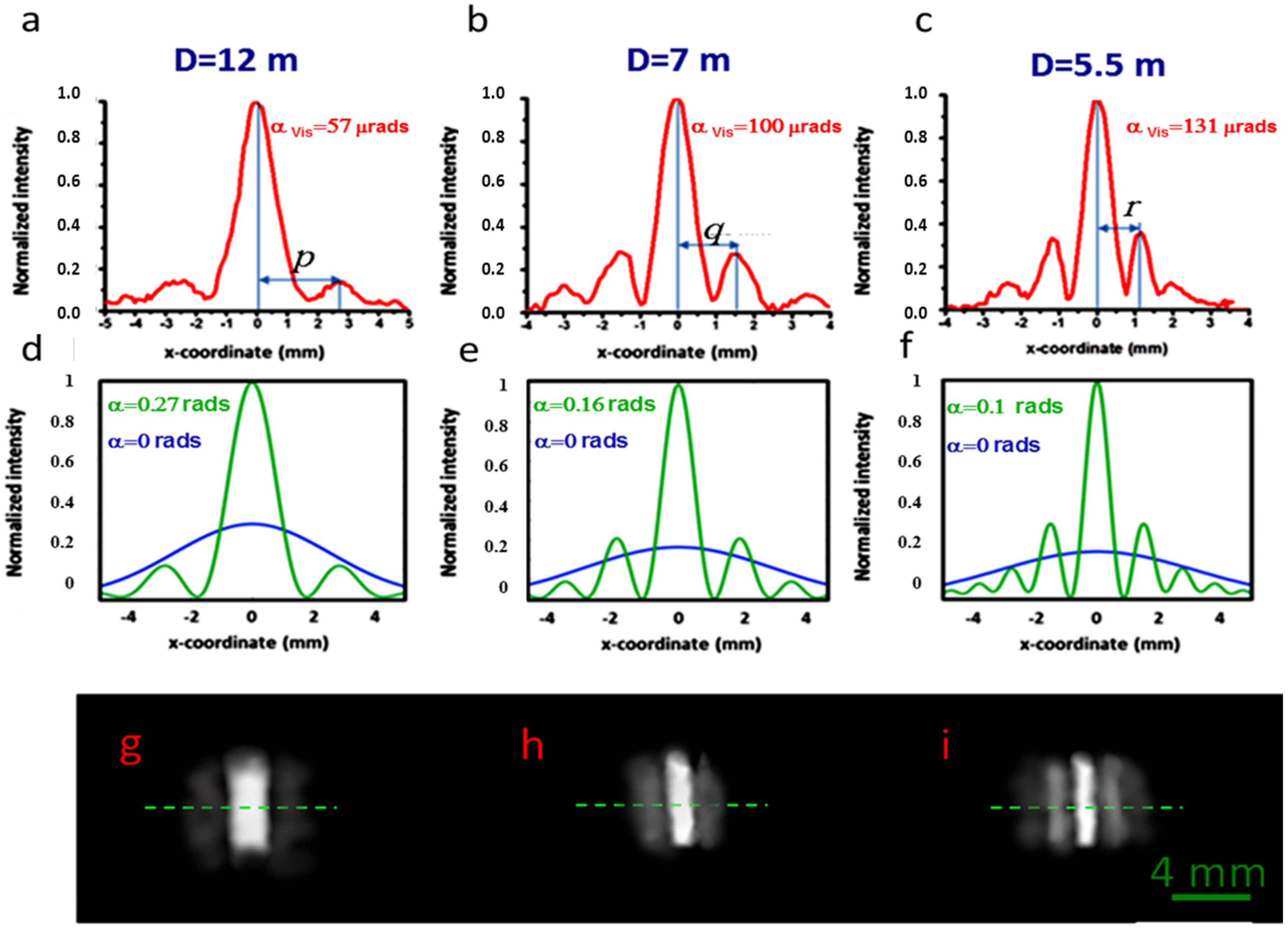
| αvis (mrads) | w (mm) | D (m) | Mλ | feq (mm) | DOF (mm) | DOFG (mm) | Dnom (m) | Δη (%) | |
|---|---|---|---|---|---|---|---|---|---|
| 0.1 THz | 57 | 1.4 | 12 | 4761 | 3.4 | 6.6 | 0.46 | 15.7 | 2.4 |
| 0.33 THz | 101 | 1.2 | 7 | 1587 | 5 | 8.5 | 0.61 | 7.9 | 0.5 |
| 0.63 THz | 131 | 0.81 | 5.5 | 762 | 6.8 | 11.5 | 0.53 | 5.2 | 0.8 |
Disclaimer/Publisher’s Note: The statements, opinions and data contained in all publications are solely those of the individual author(s) and contributor(s) and not of MDPI and/or the editor(s). MDPI and/or the editor(s) disclaim responsibility for any injury to people or property resulting from any ideas, methods, instructions or products referred to in the content. |
© 2024 by the authors. Licensee MDPI, Basel, Switzerland. This article is an open access article distributed under the terms and conditions of the Creative Commons Attribution (CC BY) license (https://creativecommons.org/licenses/by/4.0/).
Share and Cite
Margheri, G.; Del Rosso, T. Tunable Device for Long Focusing in the Sub-THz Frequency Range Based on Fresnel Mirrors. Micromachines 2024, 15, 715. https://doi.org/10.3390/mi15060715
Margheri G, Del Rosso T. Tunable Device for Long Focusing in the Sub-THz Frequency Range Based on Fresnel Mirrors. Micromachines. 2024; 15(6):715. https://doi.org/10.3390/mi15060715
Chicago/Turabian StyleMargheri, Giancarlo, and Tommaso Del Rosso. 2024. "Tunable Device for Long Focusing in the Sub-THz Frequency Range Based on Fresnel Mirrors" Micromachines 15, no. 6: 715. https://doi.org/10.3390/mi15060715