3.2. Potentiodynamic Test
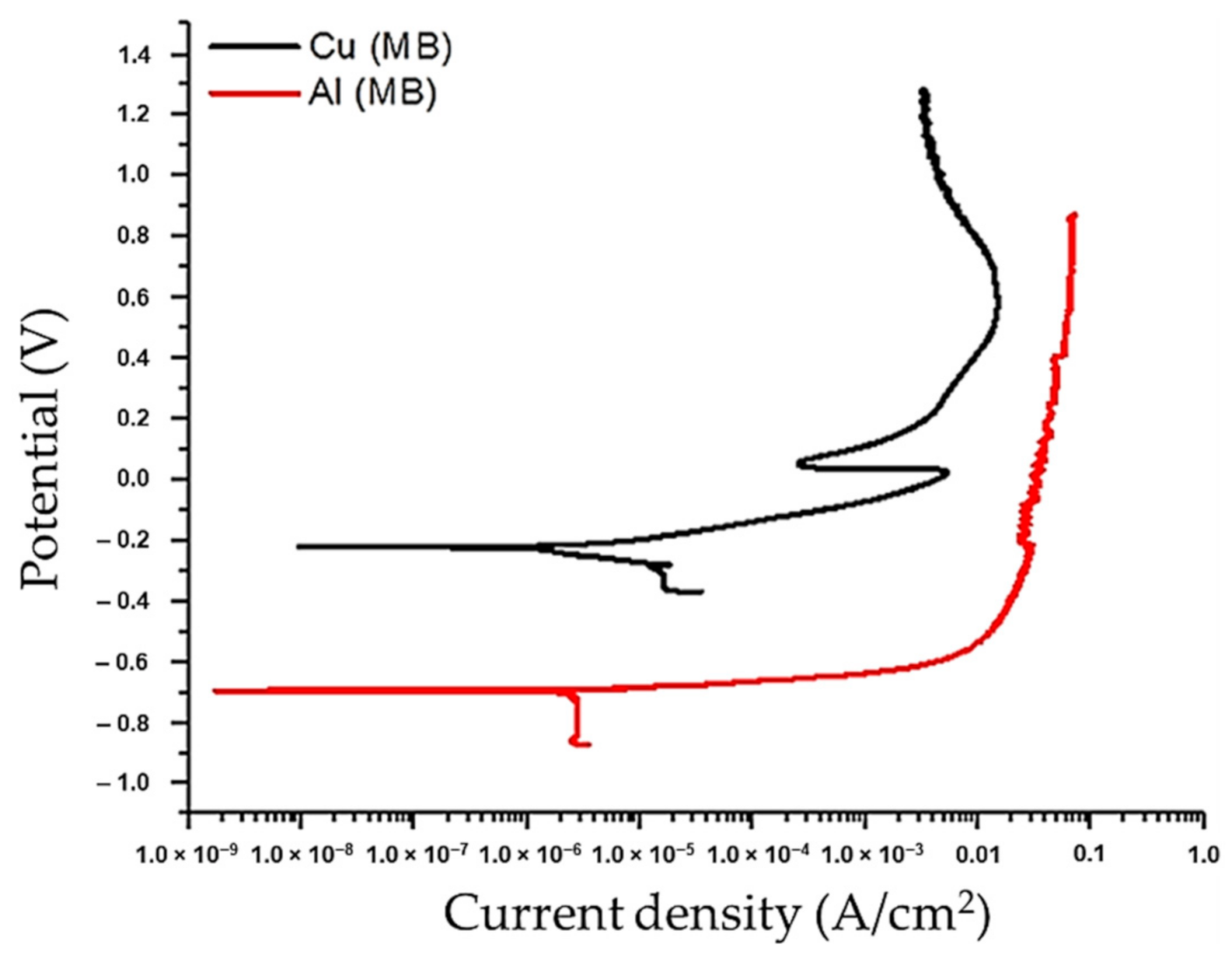
The corrosion rate for each base material was determined from the potentiodynamic curves (
Figure 4): 1.104 mpy for Al 6061-T6 and 1.364 mpy for Cu C11000. These results indicate that Al 6061-T6 has greater corrosion resistance than Cu C11000 when both materials are exposed to a NaCl solution. When aluminum comes into contact with an electrolyte, it first forms a compact and amorphous layer of aluminum oxide, mainly γ-Al
2O
3 (boehmite), a few nanometers thick. This layer will form at any temperature as soon as the solid metal touches an oxidizing medium. Covering the barrier layer is a thicker, less compacted and more porous outer layer of hydrated oxide. This second layer grows on the first following a reaction with the external environment (probably due to hydration), and its final thickness depends on the presence of physicochemical conditions (relative humidity and temperature) that favor the growth of the film [
44,
45].
The reactions that occur within the passive film when in contact with moisture or water are as follows:
According to Volkan [
45], the composition of the outer layer is a mixture of Al
2O
3 and hydrated Al
2O
3, mainly in the form of amorphous Al(OH)
3 or α-Al(OH)
3 (bayerite). This AlOOH-Al(OH)
3 outer coating is colloidal and porous, with poor corrosion resistance and cohesive properties. On the other hand, the inner layer is composed mainly of Al
2O
3 and small amounts of hydrated aluminum oxide, mainly in the form of AlOOH (boehmite). This internal Al
2O
3-AlOOH coating is continuous and corrosion resistant [
44]. Goh [
46] reported that with copper, the formation of CuCl
2 does not allow the Cu’s self-passivation, and this will inevitably increase the rate of corrosion of Cu. Moreover, Cl
− ions can act as a catalyst for copper corrosion and weaken or dissolve the stable passivation of the oxide film.
Figure 5a presents the potentiodynamic curves of the weld zones obtained at 1300 rpm and a range of traverse speeds, and
Figure 5b shows the weld zones obtained at 20 mm/min and different rotational speeds. In both cases, a similar behavior to that of the Al 6061-T6 is obtained, as can be seen in
Figure 5. This is because, during the FSW, the rotary tool was completely immersed in the aluminum plate, and it only touched the surface of the copper plate. The corrosion potential ranged from 677.63 to 700.53 mV, which is probably due to the quantity and size of the copper particles dragged onto the weld surface by the rotary tool. The copper particles and aluminum matrix form a galvanic couple, and since aluminum is less noble than copper, it will tend to corrode before copper.
As
Table 3 shows, the corrosion rate has a proportional relationship with both traverse and rotational speeds. At higher traverse speeds and a constant rotational speed, the corrosion rate increases, while higher corrosion rates are obtained with higher rotational speeds and a constant traverse speed. The S1000-20 sample showed the lowest corrosion rate (0.95927 mpy), while the S1300-60 sample presented the highest corrosion rate, at around 3.451 mpy.
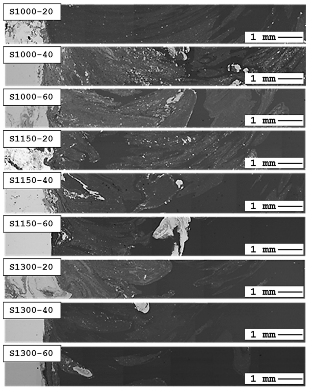
Figure 6 shows the microstructures of samples S1000-20 and S1300-60 after the corrosion tests. The weld zone’s microstructure contains equiaxed grains with copper particles at the grain boundaries. As the tool was completely inserted into the aluminum side and only had surface contact with the copper side, detachment occurred due to the heat input effect and the material flow. Stirring and plastic deformation caused the disintegration of the detached copper into small particles, which were located at the grain boundaries during the recrystallization of the weld zone.
NaCl was seen to preferentially attack the grain boundaries of aluminum, while the copper particles were subjected to no visible attacks, because copper acts as a cathode in the galvanic microcell that is formed between the copper and aluminum. In Al-Mg-Si alloys, Mg-Si particle precipitation occurs at the grain boundaries, which thus act as preferential sites for the commencement of corrosion when the alloy is exposed to a saline medium. These particles tend to be highly anodic with respect to the matrix, and they favor the activity of the galvanic couple [
47,
48,
49,
50].
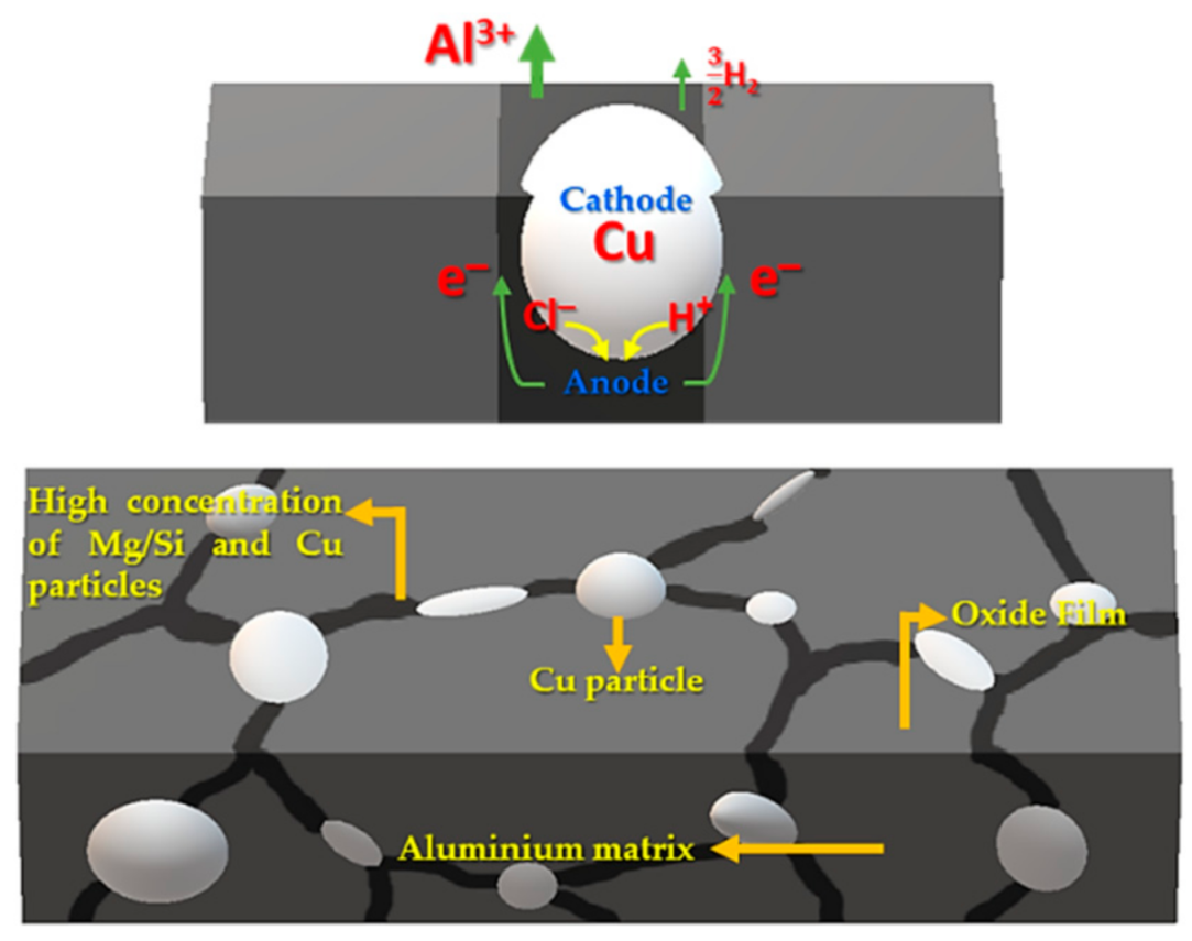
Figure 7 schematically represents the formation of a galvanic microcell between a copper particle and the grain boundaries of the aluminum alloy, which act as a cathode and an anode, respectively. The formation of these microcells favors the nucleation of pits, which gives rise to an intergranular attack within the aluminum alloy. In addition to copper particles, the IMCs that are formed during welding (previously reported by Garcia [
16]) could also act as cathodes in the formation of these microcells.
Figure 8 shows the effects of different welding conditions on the corrosion rates of all the samples. Increases in the rotational and the transverse speeds evidently increase the corrosion rate, this being greater with a higher transverse speed.
The corrosion resistance of Al-Cu welds depends on their ability to produce a uniform film of corrosion products. This film acts as a barrier between the electrolyte and the surface [
51]. The film’s uniformity improves its corrosion resistance, and depends on the distribution and size of the copper particles. Furthermore, the corrosion resistance also depends on the grain size in the weld zone.
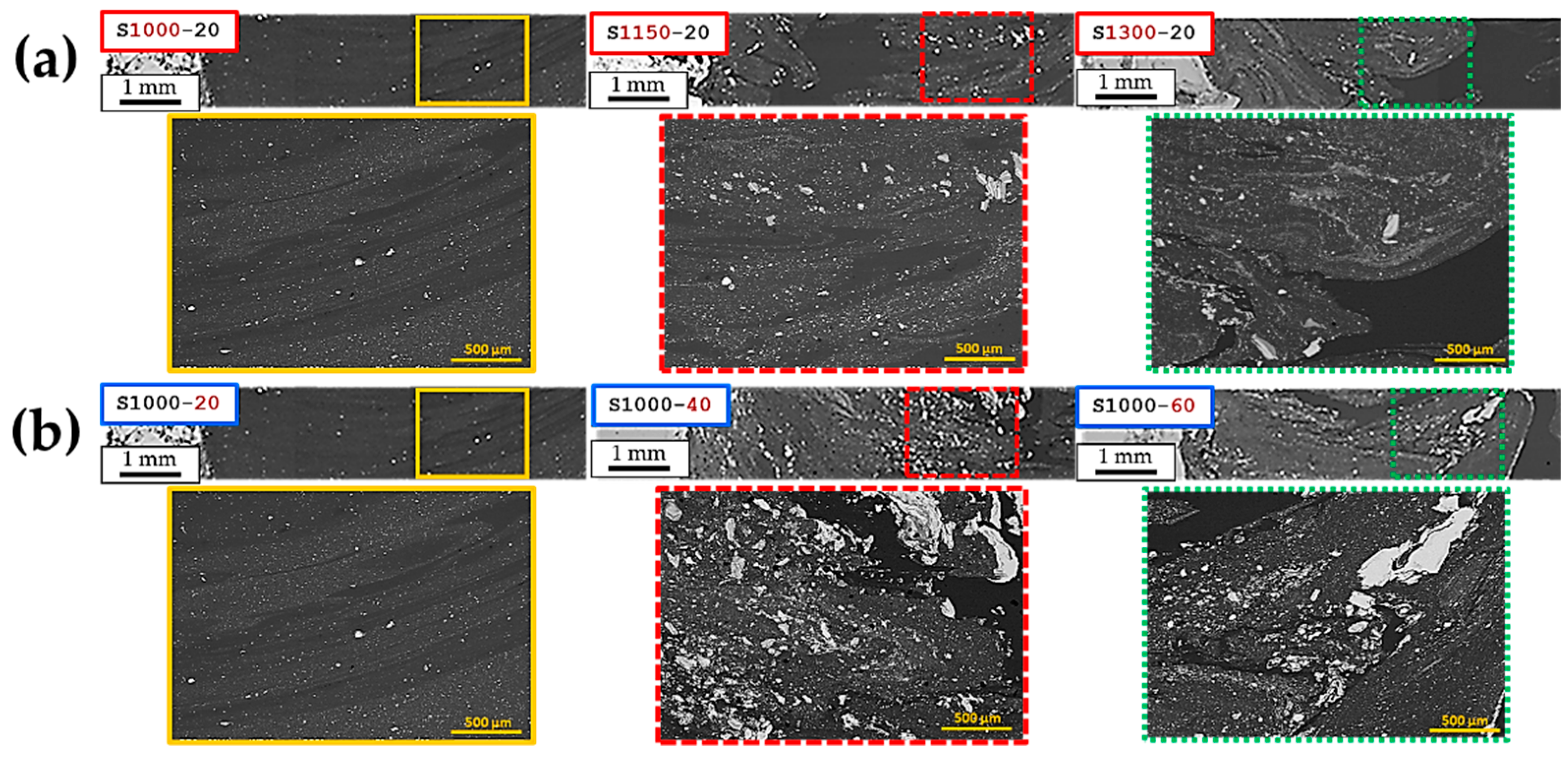
Figure 9 shows the effects of the traverse and rotational speeds on the microstructure, the grain size, and the distribution and size of the copper particles, of the welds. The increases in the rotational and traverse speeds result in an increase in the copper particles’ sizes. This increase is more noticeable for the traverse speed and is attributed to the rapid application of the heat source. Meanwhile, particle disintegration is not possible. In addition, the joint welded at 1000 rpm shows a layered flow pattern, characteristic of FSW. However, as the rotational and traverse speeds increase, this pattern deforms as a consequence of the combination of high heat input and excessive stirring in the weld zone.
These microstructural differences cause zones wherein the large potential difference aids the localized attacking of the grain boundaries and the subsequent appearance of pits [
52,
53,
54].
As the corrosion tests of the microstructures showed, the increases in rotational speed also caused an increase in the grain size as a consequence of the higher temperature during welding, which allowed grain growth during cooling. We can also see that a thickening of the anodic precipitates of Al-Mg-Si [
55,
56,
57] increases the severity of the pitting. The increase in the traverse speed causes a reduction in the grain size due to the rapid movement of the heat source through the weld, which reduces the heat retention, thus limiting the recovery and grain growth [
58]. Smaller grain sizes give rise to greater numbers of anodic sites, which aid in the formation of the galvanic couple, causing more significant surface attack [
59].
3.3. Mathematical Model
In order to develop the mathematical model, we performed three repetitions of each experiment, and the averages were determined. The model was proposed after 26 tests, and two tests were performed only for the 1300 rpm and 60 mm/min conditions. The standard deviation is one aspect of the mean of each test, which means that the experimental data oscillate close to the mean. The values of the standard deviation are , and .
The proposed model contains three degrees of freedom (dof), which are the rotational and the traverse speeds and the corrosion rate. However, it is important to consider a higher number of experiments than of dof, in order to ensure the robustness of the model. The least square method minimizes the distance between the obtained values and the proposed function, which allows the production of the curve that is most representative of the experimental values. The number of experimental repetitions (26) is higher than that of dof (3), and this is a sufficient condition to apply a mathematical model to the FSW process.
Once the average values from the corrosion rate data of the FSW process were obtained, as shown in
Table 3, an analysis of variance (ANOVA) was proposed to demonstrate the effects of welding parameters on the corrosion rate. Besides this, a mathematical model is proposed to parametrize the effects of the rotational and traverse speeds on the corrosion rate in the FSW process, which is based on a powers equation enacted via the linearization of natural logarithms.
Figure 10 shows the linear tendency between the percentile sample of each test and the corrosion rate. Therefore, a correlation study is made possible by the Pearson coefficient due to its simple implementation.
Moreover,
Table 3 demonstrates the corrosion rate achieved under different welding conditions in mpy. Based on the normal probability calculations, a Pearson (
r) correlation study is undertaken to assess the FSW’s practical implementation, and even to numerically indicate a linear relationship. The Pearson correlation should satisfy the following criteria:
where the following obtains:
Here,
is the rotational and the traverse speeds variable, and
is the corrosion rate. A strong linear relationship between
and
is guaranted when
r → −1 or
r → 1. The Pearson coefficient is computed as follows:
where
and
are the standard deviation from
and
, respectively, and
is the covariance from
and
. As such, the Pearson correlation determines the relationship between both variables.
Table 4 shows compares the rotational and traverse speeds, using a Pearson correlation matrix, following a corrosion resistance test.
Table 5 describes the types of relationship between the variables and the correlation matrices.
The significance level is the probability of being able to reject the null hypothesis when it is true. As such, the significance levels represent the probability that the confidence interval of a distribution is beyond it. The above-mentioned suggests that the contrast statistic is in the rejection zone. The significance level complements the confidence interval. As an example, if a 95% reliability study is done, then = 0.05. In another example, if a 99% reliability study is done, then = 0.01.
Table 4 shows the experimental design employed to obtain a direct relationship between the corrosion rate and the different welding parameters, where the significance level of the variables for each experimental design is
= 0.05.
As such, it is important to establish the next hypothesis for the significance level (
), as follows.
The null hypothesis:
determines that there are no significant differences in the phenomena produced by the variables. The condition is the following, in which F is the statistical Fisher distribution and is defined as the difference in the variances of sampling distribution
:
Therefore, the probability is greater than the level of significance ().
The alternative hypothesis:
determines that there are significant differences in the phenomena produced by the variables. The condition is the following:
Thus, the probability is lower than the level of significance ().
Fisher distribution concerns the statistical factor
, which indicates the relationship among the variances. When this statistical factor is close to 1, it describes a small variation between the samples. When the sample sizes
N1 and
N2 are equal to 2, the normal variances
and
define the statistical factor F, as follows:
and
The statistical Fisher distribution is
where
is a constant that depends on
and
, such that the area under the curve is equal. The database tables in [
60] are of note, wherein the distribution
is the
dof in the numerator from
and
, and
is the
dof in the numerator
.
The variation between the treatments is as follows:
where
a is the number of rows,
b is the number of columns,
xi,j are the values on the table,
is the row average,
is the column average, and
is the total average. The variation between the blocks is
while the total variation is
and the residual variation
is
where
is the total variation,
is the variation between the treatments and
is the variation between the blocks.
The mean square term between the treatments is
while the mean square term between blocks is
and the mean square term between residuals is
In addition, the term
in the hypotheses
and
at (6) and (7) is determined by
where
is related to the rotational speed, and
where
is related to the traverse speed.
According to
Table 6 and
Table 7, the alternative hypothesis
is validated for the welding parameters. Thus, the statistical analysis demonstrates the effects of the rotational and traverse speeds on the corrosion resistance. Here,
is the number of degrees of freedom in the mathematical model.
Moreover, as regards the ANOVA study, a strategy to obtain an approximation function from the data, by minimizing the sum of the residual errors of all the available data between the experimentally measured “
” and the computed “
”, is expressed as follows:
Applying the concept of the quadratic error, a regression model is proposed based on a power equation that is linearized by natural logarithms. Here,
is the corrosion (mpy),
is the rotational speed (rpm) and
is the traverse speed (mm/min).
From the natural logarithm’s properties, it is possible to linearize (21) as follows:
Then, applying the quadratic error Equation (20) to (22),
To determine the values of the coefficients
,
and
, it is necessary to find the partial derivative of (23) with respect to the coefficients
and
, which are equal to zero. This minimizes the error between the measured data and the function-computed data. The mathematical model is
and the magnitude of the residual error associated to the dependent variable is
represents the sum of the squares, which gives the average for the dependent variable y. The difference between
quantifies the reduction in the error by describing the data in terms of a linear function instead of an average value. The difference is normalized in terms of
to obtain
where
is the determination coefficient and
is the correlation coefficient. In the ideal case,
and
, and this would explain 100% of the data variability. On the contrary, when
and
, the adjustment does not offer any improvement. The standard error is formulated as follows:
where
and
are used to obtain the coefficients
,
and
in (21). Similarly,
is the total
dof, and
is the number of experiments. Therefore, to compute the
, the following equation is used:
the determination-adjusted coefficient is used to validate the degree of effectiveness of the independent variables.
Table 8 shows the results of the statistical analysis, wherein there is a direct relationship between the welding parameters and the corrosion resistance, based on the factor
. Furthermore, the corrosion resistance has a high variability as a function of the welding parameters, as is demonstrated by the factor
. The adjusted
indicates the significant influence of the input variables over the model. Finally, the error is considered too low to affect the relationship of the experimental data with the proposed model.
Figure 11 compares the experimental results and the estimated model related to the effects of the welding parameters on the corrosion rate. The model has a low absolute percentage error, and, therefore, can be utilized to obtain reliable results.
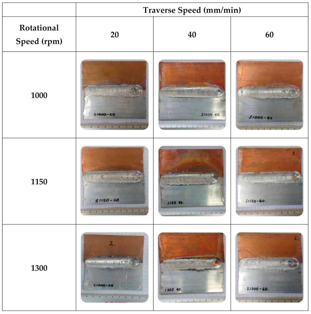
According to the color scale in
Figure 12, a traverse speed between 20 and 30 mm/min causes a small change in corrosion rate. On the other hand, a traverse speed of 20 mm/min causes greater interaction between both materials, resulting in a mixture with a larger grain size, as is shown in
Figure 3 and
Figure 6. Similar results in Al-Cu bonds have been reported by Akinlabi et al. [
61] and Rojanapanya et al. [
62], who, respectively, recommend working with traverse speeds between 20 and 50 mm/min in order to ensure metallurgical joints free of defects.
The statistical model helps quantify the effects of the rotational and traverse speeds on the corrosion rate. In addition, the statistical model avoids the need for many experiments, as the effectiveness value of the model has been variously shown to be 85% and 89.4% in terms of uncertainty.


 ,
, 


