Reduced Statistical Representation of Crystallographic Textures Based on Symmetry-Invariant Clustering of Lattice Orientations

Abstract

As proven in numerous experimental and theoretical studies, physical and mechanical properties of materials are determined by their internal structure. In the particular case of polycrystalline metals and alloys, an important role is given to the orientation distributions of crystalline lattices, or, in other words, crystallographic textures. Physically reasonable models of texture formation are highly demanded in modern Material Science and Engineering since they can provide an efficient tool for designing polycrystalline products with improved operational characteristics. Models of interest can be obtained on the basis of statistical formulations of multilevel approaches and crystal elasto–visco–plasticity theories (in particular, Taylor–Bishop–Hill models and their various modifications are appropriate here). In such a framework, a representative volume element of a polycrystal is numerically implemented as a finite aggregate of crystallites (grains or subgrains) with a homogenized response at the macro-scale. Quantitative texture analysis of this aggregate requires estimating statistically stable features of the orientation distribution. The present paper introduces a clustering-based approach for executing this task with regard to preferred orientations. The proposed procedure operates with a weighted sample of orientations representing the aggregate and divides it into clusters, i.e., disjoint subsets of close elements. The closeness criterion is supposed to be defined with the help of a special pseudometric distance, which takes rotational symmetry of the crystalline lattice into account. A specific illustrative example is provided for better understanding the developed procedure. The texture in the clustered aggregate can be described reductively in terms of effective characteristics of distinguished clusters. Several possible reduced-form representations are considered and investigated from the viewpoint of aggregating elastic properties in application to some numerically simulated textures.

1. Introduction

In a polycrystalline metal or alloy subject to severe plastic deformation, the internal structure evolves causing changes in material response at different scales. Depending on the loading process, its crystallites can rotate leading to inhomogeneity in the distribution of their lattice orientations. In such a case, it is said that a crystallographic texture is formed. This texture has significant influence on material properties at the macroscale and induces certain anisotropy in them. Texture prediction is of great interest in various simulations of technological operations since it makes possible to design materials with improved performance. A physically reasonable approach to describing quantitatively deformation-based processes with texture formation taken into consideration is to employ multilevel elasto–visco–plasticity models. Unlike common macrophenomenological theories, such models provide information on the internal state of a polycrystalline material being processed in terms of parameters characterizing key physical mechanisms (dislocation slips, grain reorientations, etc.) of inelastic deformation. Historically, this framework emerged from the crystal plasticity theories formulated in the pioneering publications of Bishop, Elam, Hill, Lin, Sachs, Taylor et al. [1,2,3,4,5,6,7,8]. By now, there are a substantial amount of works contributed in its development with improvements of constitutive equations, numerical implementations and various applications. Reviews of such works can be found, e.g., in the papers of Anand, McDowell, Roters, Trusov, Van Houtte et al. [9,10,11,12,13,14,15]. Theoretical questions related to the multilevel approach are discussed, e.g., in the publications of Busso, Luscher et al. [16,17,18]. Presently, the multilevel models of polycrystals are in widespread use for simulating deformation processes in metals and alloys. One should note that the vast majority of their computational implementations are based on the finite element method and, thus, referred as crystal plasticity finite element models (CPFEMs). Conventionally, three classes of CPFEMs can be distinguished [15]: statistical, self-consistent, and direct ones.

In statistical models, each integration point of a finite element mesh is associated with a macroscopic representative volume element (RVE) of a material. This macro-RVE is usually implemented as a polycrystalline aggregate (PA), i.e., a finite set of crystallites (which are understood as meso-RVEs) with their own values of state variables. It is worthy to remark that some approaches [19,20,21,22,23,24] deal with continuous distributions of such variables over the space of crystallite orientations. Generally speaking, fields over the space of arbitrary crystallite states can be considered instead, including the macro-RVE itself. However, obtaining numerical solutions, as a rule, relies on certain discretization schemes.

Self-consistent models, which are also referred as mean-field models, operate with grain-inclusions embedded in a matrix representing effective characteristics of a polycrystal. In recent decades, techniques based on the fast Fourier transform have been developed [25,26] to speed up computing the local responses of a material. Nonetheless, such models are still resource-intensive so their application to real problems is limited.

In direct models, each integration point corresponds to a single crystallite. Though these models are in fact one-scale (since they are formulated solely in terms of mesoscopic characteristic), they can be perceived as multi-level ones from the viewpoint of constitutive equations describing different aspects of inelastic deformation. It should be noted that such an approach is computationally even more expensive than self-consistent models.

Simulations of real deformation-based technological operations with polycrystalline materials generally require solving non-stationary geometrically non-linear boundary-value problems with a priori unknown contact conditions. Moreover, goals being pursued by practical applications (e.g., functional material design) often lead to considering inverse formulations of these problems. With purpose to make them numerically implementable (from the viewpoint of resource consumption), the use of statistical models seem to be quite perspective. In the framework of such implementations, each RVE corresponds to a PA, which usually consists of 100–1000 crystallites. Thus, the texture in a RVE is given by orientations and volume fractions of crystallites within its PA. For textured materials, it is of interest to represent orientation distribution data in a reduced manner. To do so, one should establish a compendious set of statistically estimable characteristics providing a comprehensive description of the given texture.

Quantitative description of the crystallographic texture in a RVE usually refers (explicitly or implicitly) to the concept of orientation distribution function (ODF). This function, which can be considered also as density, induces the orientation distribution measure (ODM) defining lattice volume fractions of crystallites with orientations in different subsets. Most applications operate with ODFs implemented in certain reduced forms. Common reducing approaches include series expansions, e.g., with respect to the symmetrized generalized spherical harmonics [27], the tensorial bases functions [22,28] or the empirical Karhunen–Loeve eigenfunctions [23,29,30], which refer to the proper orthogonal decomposition [31] or its simplified analogue—the method of snapshots [31,32]; all kinds of techniques based on discretizing the parameter space of lattice orientations, e.g., representations in the form of empirical ODFs, which lead to texture vectors [33] or ODF-histograms [34], or finite element approximations [21,22,23,29,30]; and the method of texture components [35,36,37,38,39,40,41]. Some of the mentioned approaches are well known in texture analysis as methods for evaluating ODFs by the inversion of diffraction pole figures [42,43]. It should be noted that expansions appropriate for statistical models, [22,27,28], usually require considering a quite large amount of series terms in order to adequately describe a sharp texture [43]. In discretization-based techniques, meshes adapted for typical textures in certain processes may be of interest. Such meshes can be obtained by identifying statistically preferred orientations (which are, in fact, local maximums of ODFs) in specially textured PAs. The method of texture components locally approximates an ODF in the neighborhoods of chosen orientations (or fibers) corresponded to these components. Since the amount and locations of the components for general textures are not known a priori, any application of the method, yet again, require preferred orientations to be identified. This task can be performed by involving some clustering techniques [44,45,46,47], which are presented in the paper.

The proposed approach is based on the statement that crystallites with close (in a certain formalizable sense) orientations contribute into aggregated material properties almost proportionally to their volumes. Such crystallites can be then grouped into a cluster, effective characteristics (conditional centers, total volume fraction of corresponded crystallites, etc.) of which can be used to describe the texture of the given PA in a reduced manner. In fact, each cluster defines a higher-density region in the space of orientations and hence can be considered as a peak-type texture component. For identifying them all, a heuristic clustering procedure is developed in this work and related ones [45,46]. It should be noted that the concept of closeness (or similarity) between elements is a crucial part in any clustering scheme. Since these elements are orientations of crystalline lattices, their rotational symmetry needs to be taken into account. This problem is resolved by introducing a symmetry-invariant pseudometric distance on the special orthogonal group, in virtue of which such orientations can be compared.

The paper is organized as follows. In Section 2, preliminaries are given: general definitions and notations are listed and a metric distance between orientations is introduced. For the sake of readability, some theoretical details of this section are placed in Appendix A and Appendix B. Section 3 is devoted to a thorough description of the proposed clustering procedure. In Section 4, examples of applying the developed procedure to reducing numerically simulated crystallographic textures are provided. Section 5 discusses adequacy of reduced texture representations and their similarities with certain statistical analogues from the viewpoint of aggregating material properties. The paper ends in Section 6 with a brief conclusion.

2. Preliminaries

Presentation of the work relies on some elements of Tensor Algebra [48,49], Theory of Groups [50] and Measure Theory [51,52]. For the sake of completeness, all necessary basic algebraic operations with tensors are listed in Appendix A. In this section, the space of crystalline lattice orientations is introduced in a formal manner and a pseudo-metrical distance between its elements is defined. Mathematical details are provided in Appendix B. Considerations related to the parametrization of such a space, its various topological properties and some statistical applications can be found in the references cited below and elsewhere [53,54].

In what follows, ${\mathbb{E}}_3$ is the three-dimensional Euclidean space over the real field, $ℝ$ (the case of the complex field, $ℂ$, is referred as ${\mathbb{E}}_3\left(ℂ\right)$), with the dot product denoted by ”$\cdot$”, and ${\mathbb{E}}_3^{\left(R\right)}$ is the space of $R$-rank tensors over ${\mathbb{E}}_3$. Let ${\mathbb{O}}^{+}\subset {\mathbb{E}}_3^{\left(2\right)}$ be the group of special orthogonal tensors. It is worthy to remind that ${\mathbb{O}}^{+}$ is not a linear subspace of ${\mathbb{E}}_3^{\left(2\right)}$ since a linear combination of special orthogonal tensors generally is not a special orthogonal tensor. By definition, each $\mathbf{r}\in {\mathbb{O}}^{+}$ represents some rotation transform, $r:{\mathbb{E}}_3\to {\mathbb{E}}_3$:

$$r\left[v\right]=\mathbf{r}\cdot v.$$

(1)

The choice of a parametrization on ${\mathbb{O}}^{+}$ does not play a significant role in the paper. However, an opportunity to specify explicitly axes and angles of rotations as, e.g., in the case of quaternions [55] or neo-Eulerian parameters [22], seems to be of interest. The rotation around an axis vector $a\in {\mathbb{E}}_3$ by an angle $\alpha \in ℝ$ is further denoted by the tensor ${\mathbf{R}}_a^{\alpha }\in {\mathbb{O}}^{+}$.

Within this work, ${\mathbb{O}}^{+}$ is treated as the space of all orientations for a (three-dimensional) crystalline lattice. Each orientation can be described by a rotation to an actual position from some reference one, which is supposed to be the same for all orientations under consideration. In other words, if a laboratory coordinate system with the bi-orthogonal normalized basis vectors $l_1,l_2,l_3\in {\mathbb{E}}_3$ is fixed, then an arbitrary lattice orientation of a crystallite can be specified by the tensor $\mathbf{o}\in {\mathbb{O}}^{+}$ which rotates, under (1), these vectors to same-handed bi-orthogonal normalized basis vectors, $k_1,k_2,k_3\in {\mathbb{E}}_3$, rigidly bound to the crystallite:

$$\mathbf{o}=k_i{l}_i.$$

(2)

With this in mind, tensors of ${\mathbb{O}}^{+}$ are also termed as just orientations.

An important question, especially in the context of clustering, is the way in which closeness of two arbitrary orientations, ${\mathbf{o}}^{\mathrm{I}},{\mathbf{o}}^{\mathrm{II}}\in {\mathbb{O}}^{+}$, can be measured. Particular interest is addressed to the rotation between them, i.e., ${\mathbf{o}}^{\mathrm{II}}\cdot {\mathbf{o}}^{\mathrm{I}\hspace{0.17em}⊺}$ (from ${\mathbf{o}}^{\mathrm{I}}$ to ${\mathbf{o}}^{\mathrm{II}}$) or ${\mathbf{o}}^{\mathrm{I}}\cdot {\mathbf{o}}^{\mathrm{II}\hspace{0.17em}⊺}$ (vice versa), and the corresponding angle. When restricted to be in $\left[0,\mathsf{\pi }\right]$, this angle is actually the value of the metric distance $d:{\mathbb{O}}^{+}\times {\mathbb{O}}^{+}\to \left[0,\mathsf{\pi }\right]$ induced by the natural Riemann metrics. In terms of angles $\alpha ,\beta \in \left[0,\mathsf{\pi }\right]$ and axes $a,b\in {\mathbb{E}}_3$ of orientations being compared, $d$ can be represented as [41]:

$$d\left[{\mathbf{R}}_a^{\alpha },{\mathbf{R}}_b^{\beta }\right]=2\arccos \left|\cos \frac{\alpha }{2}\cos \frac{\beta }{2}+\sin \frac{\alpha }{2}\sin \frac{\beta }{2}a\cdot b\right|.$$

(3)

This expression can be computationally efficient when the quaternion-based [55] or Rodrigues [22] parametrizations is used on ${\mathbb{O}}^{+}$.

As it is already mentioned above, orientations of crystal lattices are of interest in this work. Since each lattice is characterized by a certain symmetry type, there are crystallographically indistinguishable orientations in ${\mathbb{O}}^{+}$. In other words, if ${\mathbb{S}}^{+}\subset {\mathbb{O}}^{+}$ is a rotational symmetry group of a given lattice in its reference orientation, then an arbitrary orientation $\mathbf{o}\in {\mathbb{O}}^{+}$ of this lattice is symmetrically equivalent to all $\mathbf{o}\cdot \mathbf{s}$ such that $\mathbf{s}\in {\mathbb{S}}^{+}$. Surely, a reasonable closeness criterion for lattice orientations should be introduced with this feature taken into consideration. In order to do so for clustering purposes, one can use the pseudometric distance $d_{{\mathbb{S}}^{+}}:{\mathbb{O}}^{+}\times {\mathbb{O}}^{+}\to \left[0,\mathsf{\pi }\right]$ defined as follows:

$$\begin{array}{c}{d}_{{\mathbb{S}}^{+}}\left[{\mathbf{R}}_a^{\alpha },{\mathbf{R}}_b^{\beta }\right]=2\underset{{\mathbf{R}}_c^{\gamma }\in {\mathbb{S}}^{+}}{\min }\arccos |\cos \frac{\gamma }{2}\left(\cos \frac{\alpha }{2}\cos \frac{\beta }{2}+\sin \frac{\alpha }{2}\sin \frac{\beta }{2}a\cdot b\right)\\ -\sin \frac{\gamma }{2}\mathbf{c}\cdot \left(\sin \frac{\alpha }{2}\cos \frac{\beta }{2}a-\cos \frac{\alpha }{2}\sin \frac{\beta }{2}b+\sin \frac{\alpha }{2}\sin \frac{\beta }{2}a\times b\right)|.\end{array}$$

(4)

It is possible to show that $d_{{\mathbb{S}}^{+}}\left[{\mathbf{o}}^{\mathrm{I}},{\mathbf{o}}^{\mathrm{II}}\right]$ determines the minimal angle of rotations between ${\mathbf{o}}^{\mathrm{I}}$ and ${\mathbb{S}}^{+}$-equivalent analogues of ${\mathbf{o}}^{\mathrm{II}}$. Thus, $d_{{\mathbb{S}}^{+}}\left[{\mathbf{o}}^{\mathrm{I}},{\mathbf{o}}^{\mathrm{II}}\right]=0$ holds if and only if ${\mathbf{o}}^{\mathrm{I}}$ and ${\mathbf{o}}^{\mathrm{II}}$ are ${\mathbb{S}}^{+}$-equivalent to each other.

To eliminate non-uniqueness in the description of lattice orientations, one can narrow ${\mathbb{O}}^{+}$ to a subset which contains exactly one orientation from each ${\mathbb{S}}^{+}$-equivalence class. The closure of such a subset is called a fundamental domain for ${\mathbb{S}}^{+}$. As for the representative elements, orientations with the least angles can be chosen in these classes [56]. The corresponding fundamental domain is further denoted by the subset ${\mathcal{O}}_{{\mathbb{S}}^{+}}^{+}\subset {\mathbb{O}}^{+}$.

Let ${\mathfrak{O}}^{+}$ be the Borel sigma-algebra on ${\mathbb{O}}^{+}$. Since, in what follows, ${\mathbb{O}}^{+}$ is treated as the space of orientations, a mapping $F:{\mathfrak{O}}^{+}\to \left[0,1\right]$ is referenced as an orientation distribution measure (ODM). The ODM identical to the normalized Haar measure [51] is further denoted by $U$. For arbitrary $\left[{\mathbf{R}}_a^{\alpha }\right]$ with $\alpha \in \left[0,\mathsf{\pi }\right]$ and $a\in {\mathbb{E}}_3$, the corresponding invariant infinitesimal volume element, $\mathrm{d}U\left[{\mathbf{R}}_a^{\alpha }\right]$, is given by [57]

$$\mathrm{d}U\left[{\mathbf{R}}_a^{\alpha }\right]=\frac{1}{4{\mathsf{\pi }}^2}\left(1-\cos \alpha \right)\mathrm{d}\alpha \mathrm{d}S\left[a\right],$$

(5)

where $\mathrm{d}S\left[a\right]$ is the area element of the unit sphere at the head point of $a$. By introducing special coordinate systems on ${\mathbb{O}}^{+}$, one can obtain volumetrically homogeneous parameter spaces for representing orientations. e.g., among neo-Eulerian spaces, such one is provided by homochoric coordinates [22]. It is worthy to mention that the spaces of Eulerian angles or angles specifying axis directions and rotation magnitudes are not homogeneous in this sense.

By definition, $F\left[\mathcal{O}\right]$ determines the volume fraction of a crystal lattice, orientations of which are in $\mathcal{O}\in {\mathfrak{O}}^{+}$. If F is absolutely continuous [51] with respect to $U$, then it has the Radon–Nikodym derivative, $f:{\mathbb{O}}^{+}\to \left[0,+\infty \right)$, so that

$$F\left[\mathcal{O}\right]={\displaystyle \underset{o\in \mathcal{O}}{\int }f\left[\mathbf{o}\right]}\mathrm{d}U\left[\mathbf{o}\right].$$

(6)

Such a function is defined up to $U$-null set and termed as an orientation distribution function (or density; ODF), e.g., the ODF, $u$, corresponding to $U$ is a constant:

$$u\left[\mathbf{o}\right]=1;$$

(7)

it is also understood as the density of uniformly (i.e., equiprobable) distributed orientations. One should note that, in most applications, exactly ODFs are being considered. However, ODMs emerging in this work are not continuous in the given sense, so this term cannot be used in a rigorous manner. A simple example of such ODMs is the Dirac measure [52]. In what follows, ${\Delta }_{\mathbf{o}}$ denotes the Dirac measure concentrated at $\mathbf{o}\in {\mathbb{O}}^{+}$, which is defined by

$${\Delta }_{\mathbf{o}}\left[\mathcal{O}\right]=\{\begin{array}{l}1,\hspace{1em}\mathbf{o}\in \mathcal{O};\\ 0,\hspace{1em}\mathbf{o}\notin \mathcal{O}.\end{array}$$

(8)

Due to ambiguity caused by symmetrically equivalent orientations, an ODM cannot be determined uniquely for every crystallographically non-uniform distribution. Given a symmetry group ${\mathbb{S}}^{+}$, this feature can be resolved, e.g., by imposing the following invariance conditions on each ODM, $F$:

$$F\left[\mathcal{O}\cdot \mathbf{s}\right]=F\left[\mathcal{O}\right],$$

(9)

where $\mathcal{O}\in {\mathfrak{O}}^{+}$ and $\mathbf{s}\in {\mathbb{S}}^{+}$. Note that, in such a case, the domain of $F$ can be reduced to the Borel sigma-algebra on ${\mathcal{O}}_{{\mathbb{S}}^{+}}^{+}$. Since it is always possible to obtain a ${\mathbb{S}}^{+}$-invariant analogue of $F$ by averaging over ${\mathbb{S}}^{+}$ [50], restrictions of the form (9) are not applied to ODMs in the paper.

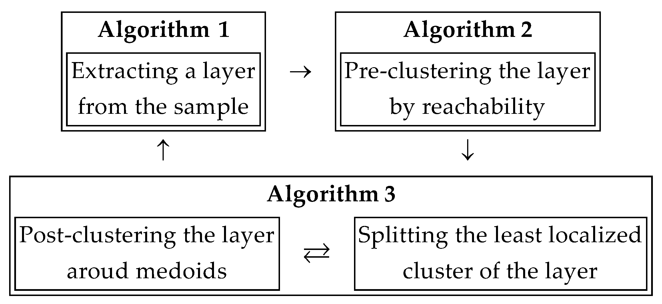
3. Crystallographic Texture Clustering

The following problem is considered in this section. Given a set of lattice orientations with known volume fractions of crystallites sharing same symmetry, split it into disjoint subsets such that elements of one subset are close to each other. Such a splitting is understood as crystallographic texture clustering (CTC) while the mentioned subsets are termed as clusters. In this work, CTC is of interest for identifying peak-type texture components in a PA.

Consider a single-phased PA of N crystallites with the rotational symmetry group ${\mathbb{S}}^{+}$, volume fractions $f_1,\dots ,f_N\in \left[0,1\right]$ (such that ${\displaystyle \sum _{n=1}^N{f}_n}=1$) and lattice orientations ${\mathbf{o}}_1,\dots ,{\mathbf{o}}_N\in {\mathbb{O}}^{+}$. For solving the CTC problem in question, an approach based on comparing exclusively orientations of the PA seems to be quite performant. In this connection, it is reasonable to introduce the so-called misorientation matrix, $D$ (of $N\times N$ size):

$$D_{m\hspace{0.17em}n}=d\left[{\mathbf{o}}_m,{\mathbf{o}}_n\right].$$

(10)

This is a symmetric matrix with main-diagonal elements equal to 0. A wide class of abstract clustering techniques can be executed by operating with only such an object (and, probably, corresponding fractions as well). The CTC procedure proposed in this paper shares common approaches with some well-known clustering algorithms [58,59], but also introduces certain modifications and generalizations (onto the case of unequal volume fractions).

In what follows in this section, main steps of the CTC procedure are demonstrated on the special sample of $N=300$ orientations: ${\mathbf{R}}_a^{{\alpha }_1},\dots ,{\mathbf{R}}_a^{{\alpha }_N}$, which are parametrized by the same axis $a\in {\mathbb{E}}_3$ and various angles ${\alpha }_1,\dots ,{\alpha }_N\in \left[0,\mathsf{\pi }\right]$ marked on Figure 1. For simplicity, all volume fractions are supposed to be equal to each other; hence, $f_n=N^{-1}=3.(3)\cdot {10}^{-3}$, $n\in \overline{1,N}$. The artificial symmetry with the non-trivial group ${\mathbb{S}}^{+}=\left\{\mathbf{I},{\mathbf{R}}_a^{\mathsf{\pi }}\right\}$ is set in this example. Thus, in terms of a geometric analogy, elements of the exemplary sample can be treated as orientations of straight lines in the plane orthogonal to $a$.

In the case of general textures, clusters are quite suppositional and their exact amount is not known a priori. To proceed correctly with clustering, it seems reasonable to identify most densely located orientations. Such a density can be introduced with the help of certain weights attributed to the orientations. For each orientation, the weight is equal to the total volume fraction of crystallites with orientations within its some pseudometric neighborhood. Note that for small enough neighborhoods the mentioned weights and fractions are identical. Weights (${\phi }_1,\dots ,{\phi }_N$) obtained for the exemplary sample of orientations are presented in Figure 2.

The step described above is equivalent to the evaluation of an especially mollified ODF at certain orientations. Indeed, let $m$ be the mollifying function of the form

$$m\left[{\mathbf{o}}^{\mathrm{I}},{\mathbf{o}}^{\mathrm{II}}\right]=\{\begin{array}{l}{\left(U\left[{ℬ}_{{\mathbf{o}}^{\mathrm{II}}}^{\omega }\right]\right)}^{-1},\hspace{1em}{\mathbf{o}}^{\mathrm{I}}\in {ℬ}_{{\mathbf{o}}^{\mathrm{II}}}^{\omega },\\ 0,\hspace{1em}{\mathbf{o}}^{\mathrm{I}}\notin {ℬ}_{{\mathbf{o}}^{\mathrm{II}}}^{\omega },\end{array}$$

(11)

where ${ℬ}_{\mathbf{o}}^{\omega }$ is the closed pseudometric ball centered at $\mathbf{o}\in {\mathbb{O}}^{+}$ of a radius $\omega >0$:

$${ℬ}_{\mathbf{o}}^{\omega }=\left\{{\mathbf{o}}^{\mathrm{I}}\in {\mathbb{O}}^{+}|\hspace{0.17em}{d}_{{\mathbb{S}}^{+}}\left[\mathbf{o},{\mathbf{o}}^{\mathrm{I}}\right]\le \omega \right\}.$$

(12)

The PA-induced ODM, $F$, is given by

$$F={\displaystyle \sum _{n=1}^N{f}_n{\Delta }_{{\mathbf{o}}_n}}.$$

(13)

Mollifying it using $m$ leads to the ODF $f^{\mathrm{m}}$:

$$f^{\mathrm{m}}\left[\mathbf{o}\right]={\displaystyle \underset{o^{\prime }\in {\mathbb{O}}^{+}}{\int }m\left[\mathbf{o},{\mathbf{o}}^{\mathrm{I}}\right]\mathrm{d}F}\left[{\mathbf{o}}^{\mathrm{I}}\right]={\displaystyle \sum _{n=1}^N{f}_{n}m\left[\mathbf{o},{\mathbf{o}}_n\right]},$$

(14)

which returns the measure-related volume fractions of crystallites with orientations within the pseudometric $\omega$-neighborhood of its argument. In the case when not the whole sample of orientations is taken into consideration, one should mollify only the sum of corresponding terms from (13). Note that practically reasonable values of $\omega$ are small enough to ensure that such neighborhood does not contain symmetrically equivalent orientations. If so, then this neighborhood can be treated as a metric one, which is defined with $d$ instead of $d_{{\mathbb{S}}^{+}}$ in (12). For this case, it is easy to derive that [53]:

$$U\left[{ℬ}_{\mathbf{o}}^{\omega }\right]=\frac{\left|{\mathbb{S}}^{+}\right|}{\mathsf{\pi }}\left(\omega -\sin \omega \right),\hspace{1em}{ℬ}_{\mathbf{o}}^{\omega }\subset {\mathcal{O}}_{{\mathbb{S}}^{+}}^{+}\cdot \mathbf{o}.$$

(15)

Hereinafter, $\left|\mathcal{X}\right|$ denotes the amount of elements in a finite set $\mathcal{X}$.

The union of the densest neighborhoods forms a layer, which usually can be decomposed into distant (from each other) subsets of orientations. It is natural to consider these subsets as clusters. Appropriate techniques to identify them all within the layer are based on a reachability relation between orientations. Herein, the reachability is understood as the transitive closure of a adjacency relation, which can be introduced through operations over $D$ and $f_1,\dots ,f_N$. A possible formalization of such an approach is presented below in Algorithms 1 and 2.

Algorithm 1. Extracting a layer from a sample.
Parameters:
•  $\mathcal{S}$, the index set defining the sample of orientations;
•  $\omega$, the radius of pseudometric neighborhoods used in mollifying;
•  $\phi$, the total fraction of the sample orientations in a neighborhood above which its content should be included in the layer.
1.  For each sample orientation, add the indexes of other sample orientations within its neighborhood to a set:
${\mathcal{N}}_n=\left\{m\in \mathcal{S}|D_{m\hspace{0.17em}n}\le \omega \right\},\hspace{1em}n\in \mathcal{S}$.	(16)
2.  For each sample orientation, calculate its weight, i.e., the total fraction of the sample orientations within its neighborhood:
${\phi }_n={\displaystyle \sum _{m\in {\mathcal{N}}_n}{f}_m},\hspace{1em}n\in \mathcal{S}$.	(17)
3.  Add the indexes of the sample orientations within sufficiently dense neighborhoods to a set:
$\mathcal{V}={\displaystyle \underset{n\in {\mathcal{S}}^{\prime }}{\cup }{\mathcal{N}}_n},\hspace{1em}{\mathcal{S}}^{\prime }=\left\{n\in \mathcal{S}\hspace{0.17em}|\hspace{0.17em}{\phi }_n>\phi \right\}.$	(18)

Algorithm 1 allows a layer to be extracted with only a sample of orientations and corresponding fractions being considered. These orientations are supposed to be specified by some set of their indexes in the PA, $\mathcal{S}$ (e.g., the whole sample is given by $\mathcal{S}=\{1,\dots ,N$). The layer is defined as the union of neighborhoods centered at orientations with weights above a certain level, φ. There are different ways to set its value; in the example shown in Figure 3, $\phi$ is chosen among “locally maximal” weights, which are computed as the ones satisfying

$${\phi }_n=\underset{m\in {\mathcal{N}}_n}{\max }{\phi }_m,\hspace{1em}n\in \mathcal{S}.$$

(19)

In general, each layer contains orientations with weights above a set level as well as orientations with weights equal or below it. Their subsets are further referenced as “core” and “periphery”, respectively.

Algorithm 2. Pre-clustering a layer by reachability.

Parameters:

•  $\epsilon$, the pseudometric distance between two orientations equal or below which they are considered as adjacent ones.

1.  Add the index pairs for close orientations within the layer to a set (of edges):   $ℰ=\left\{\left(m,n\right)\in \mathcal{V}\times \mathcal{V}\hspace{0.17em}|\hspace{0.17em}{D}_{m\hspace{0.17em}n}\le \epsilon \right\}$                                 (20)

2.  Divide the graph $\left(\mathcal{V},ℰ\right)$ into the maximal connected subgraphs   $\left({\mathcal{V}}_1,{ℰ}_1\right),\dots ,\left({\mathcal{V}}_K,{ℰ}_K\right)$.

Algorithm 2 supposes that two orientations are adjacent if they are close enough to each other in terms of $d_{{\mathbb{S}}^{+}}$. In this case, $\epsilon$ defines the lower bound for the distance between orientations of different clusters. There are also complicated variants of this relation, e.g., such ones which take intersection of corresponding neighborhoods into consideration. An example of clustering results for the described algorithm is given in Figure 4.

As an option for Algorithm 2, only core orientations of a layer being clustered can be taken into consideration. Each peripheral orientation then should be assigned to the least-distant cluster. In such a case, the combination of Algorithms 1 and 2 is a sort of so-called density-based spatial clustering of applications with noise (DBSCAN) [60]. However, from the viewpoint of the complete CTC procedure, it seems reasonable to encapsulate their operational sequences.

With purpose to obtain well-localized clusters, one can employ additionally the medoid-based clustering. In common applications, the medoid of a finite set is understood as its element, such that the mean distance from this element to other elements in the set is minimal. When being applied to sets of orientations, this concept does not take into consideration volume fractions of corresponded crystallites and, therefore, should be modified. Note that, if all fractions for a given sample share a common factor, then this sample can be replaced by another one with equal fractions and repeating orientations. In such a connection, the following definition seems to be appropriate. An orientation of a finite set is its medoid if the mean pseudometric fraction-weighted distance from this orientation to other orientations of the set is minimal.

In what follows, “←” denotes the assignment operation. Algorithm 3, which is presented below, performs the medoid-based clustering by alternating between determining medoids of current clusters and reassigning each orientation to the cluster with the closest medoid [58]. Given a fixed number of clusters, $K$, this subprocedure can be treated as a heuristic strategy for solving the discrete optimization problem: find index subsets ${\mathcal{C}}_1,\dots ,{\mathcal{C}}_K\subset \mathcal{S}$ (or some Boolean variables describing the orientation-cluster assignment) and indexes $m_1,\dots ,m_K\in \overline{1,N}$ such that the objective

$$J_K={\displaystyle \sum _{k=1}^K{\displaystyle \sum _{n\in {\mathcal{C}}_k}{f}_n{D}_{m_k\hspace{0.17em}n}}}$$

(21)

reaches its minimum and wherein

$${\displaystyle \underset{k=1}{\overset{K}{\cup }}{\mathcal{C}}_k}=\mathcal{S},$$

(22)

$${\mathcal{C}}_j\cap {\mathcal{C}}_k=\varnothing ,\hspace{1em}j\ne k,\hspace{1em}j,k\in \overline{1,K},$$

(23)

$$m_k\in {\mathcal{C}}_k,\hspace{1em}k\in \overline{1,K}.$$

(24)

In fact, (21) gives an internal criterion of clustering quality. One should note that this approach provides generally only a suboptimal (i.e., unimprovable by any further iterations) solution. There are also other possible optimization techniques; e.g., the alternative algorithm [61] or the combinatorial global minimization method [62]. Optional steps can be included to control sizes or localizations of clusters being obtained. In Algorithm 3, it is proposed to split (in a heuristic manner) the least localized cluster in half with the medoid-based clustering subprocedure being repeated after each splitting.

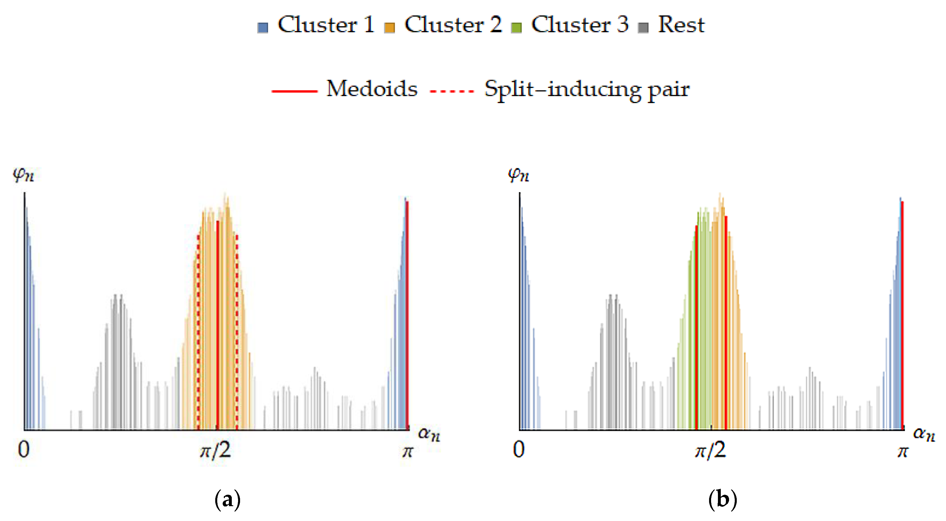
Algorithm 3. Post-clustering a layer around medoids and splitting the least localized clusters.
•  δ, the mean pseudometric deviation of cluster orientations from the medoid equal or above which the cluster should be split.
1.  For each initial cluster, find its medoid:
$m_k\leftarrow \underset{m\in {\mathcal{V}}_k}{\arg \min }{\displaystyle \sum _{n\in {\mathcal{V}}_k}{f}_n{D}_{m\hspace{0.17em}n}},\hspace{1em}k\in \overline{1,K}$	(25)
2.  For each current medoid, update the corresponding cluster by reassigning orientations to which this medoid is the closest one (among other medoids):
${\mathcal{C}}_k\leftarrow \left\{n\in \mathcal{V}\hspace{0.17em}|\hspace{0.17em}{D}_{n\hspace{0.17em}{m}_k}=\underset{j\in \overline{1,K}}{\min }{D}_{n\hspace{0.17em}{m}_j}\right\},\hspace{1em}k\in \overline{1,K}$	(26)
3.  For each current cluster, update its medoid:
$m_k\leftarrow \underset{m\in {\mathcal{C}}_k}{\arg \min }{\displaystyle \sum _{n\in {\mathcal{C}}_k}{f}_n{D}_{m\hspace{0.17em}n}},\hspace{1em}k\in \overline{1,K}$	(27)
4.  If at least one of $m_1,\dots ,m_K$ is changed at Step 3, go to Step 2.
5.  Find the cluster with the largest fraction-weighted mean pseudometric deviation of its orientations from the medoid:
$\widehat{k}\leftarrow \underset{n\in \overline{1,K}}{\arg \max }\frac{{\displaystyle \sum _{n\in {\mathcal{C}}_k}{f}_n{D}_{n\hspace{0.17em}{m}_k}}}{\left|{\mathcal{C}}_k\right|}$	(28)
6.  If the cluster determined by Step 5 is not well enough localized, i.e.,
$\frac{{\displaystyle \sum _{n\in {\mathcal{C}}_{\widehat{k}}}{f}_n{D}_{n\hspace{0.17em}{m}_{\widehat{k}}}}}{\left|{\mathcal{C}}_{\widehat{k}}\right|}\ge \delta$	(29)
6.1.  Replace its medoid by the pair of orientations with the largest weighted distance (with the amount of clusters increased by one):
$K\leftarrow K+1$	(30)
$\left(m_{\widehat{k}},m_K\right)\leftarrow \underset{\left(m,n\right)\in {\mathcal{C}}_{\widehat{k}}\times {\mathcal{C}}_{\widehat{k}}}{\arg \max }\left({\phi }_m{\phi }_n{D}_{mn}\right)$	(31)
6.2.  Go to Step 2.

Rigorously, weights used in (31) should be recalculated with only orientations of the layer (i.e., without orientations of the rest sample) being taken into consideration. However, such a recalculation does not affect core orientations, among which the medoids of split-induced clusters will be found most likely.

Convergence of Algorithm 3 is guaranteed by the fact that (21) cannot increase during Steps 2 and 3 while the non-decreasing at Step 6 amount of clusters is limited by the amount of orientations. However, iterations required for convergence and solution quality depend heavily on initial clusters (or medoids) used in the algorithm as a first approximation. Estimates for them are just being provided by Algorithm 2, so the corresponding stage is termed as “pre-clustering”. In its turn, Algorithm 3 refines the partitioning obtained in such a way and therefore is referenced as “post-clustering”. Figure 5 illustrates results of this algorithm in application to the example being tracked.

A layer extracted by Algorithm 1 and successively clustered by Algorithms 2 and 3 is then excluded from the sample. After that, the remaining sample is used for obtaining the next layer to be clustered. These steps are executed until there are no orientations left in the sample. The complete operation sequence with the whole sample being initial one is described briefly in Algorithm 4 and schemed in Figure 6. Note that it is algorithmically possible to separate sample layering from clustering so each layer can be procedured independently.

Algorithm 4. Clustering the whole sample.

1. $\mathcal{S}\leftarrow \left\{1,\dots ,N\right\}$.

2. $L\leftarrow 0$.

3. Set $\omega$ and $\phi$ an execute Algorithm 1.

4. $L\leftarrow L+1$.

5. $S\leftarrow S\backslash \mathrm{V}$.

6. Set $\epsilon$ and execute Algorithm 2.

7. Set $\delta$ and execute Algorithm 3.

8. $K_L\leftarrow K$.

9. $\left({\mathcal{C}}_{L\hspace{0.17em}k},m_{L\hspace{0.17em}k}\right)\leftarrow \left({\mathcal{C}}_k,m_k\right),\hspace{1em}k\in \overline{1,K_L}$.

10. If $\mathcal{S}\ne \varnothing$ then go to Step 3.

As a result, Algorithm 4 returns the multilevel index lists of cluster orientations and corresponding medoids:

$$\left\{\left\{{\mathcal{C}}_{1\hspace{0.17em}1},\dots ,{\mathcal{C}}_{1\hspace{0.17em}{K}_1}\right\},\dots ,\left\{{\mathcal{C}}_{L\hspace{0.17em}1},\dots ,{\mathcal{C}}_{L\hspace{0.17em}{K}_L}\right\}\right\};$$

$$\left\{\left\{m_{1\hspace{0.17em}1},\dots ,m_{1\hspace{0.17em}{K}_1}\right\},\dots ,\left\{m_{L\hspace{0.17em}1},\dots ,m_{L\hspace{0.17em}{K}_L}\right\}\right\}.$$

On the basis of such data, various reduced representations of crystallographic textures can be constructed for their further analysis. Note that orientations in the initial sample are not assumed to be within any fundamental domain. However, for possible visualization purposes, it is reasonable to preliminary project them onto ${\mathcal{O}}_{{\mathbb{S}}^{+}}^{+}$.

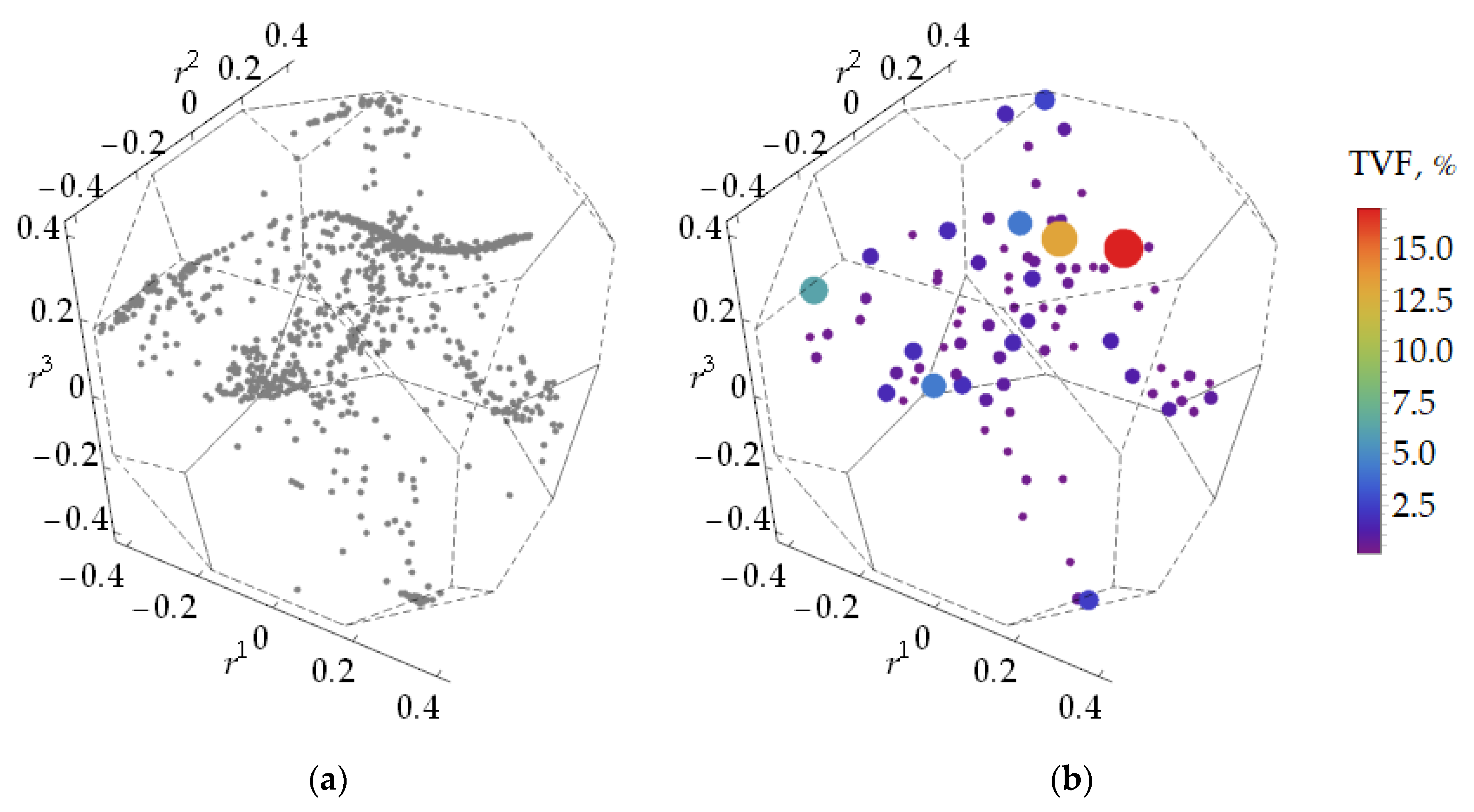
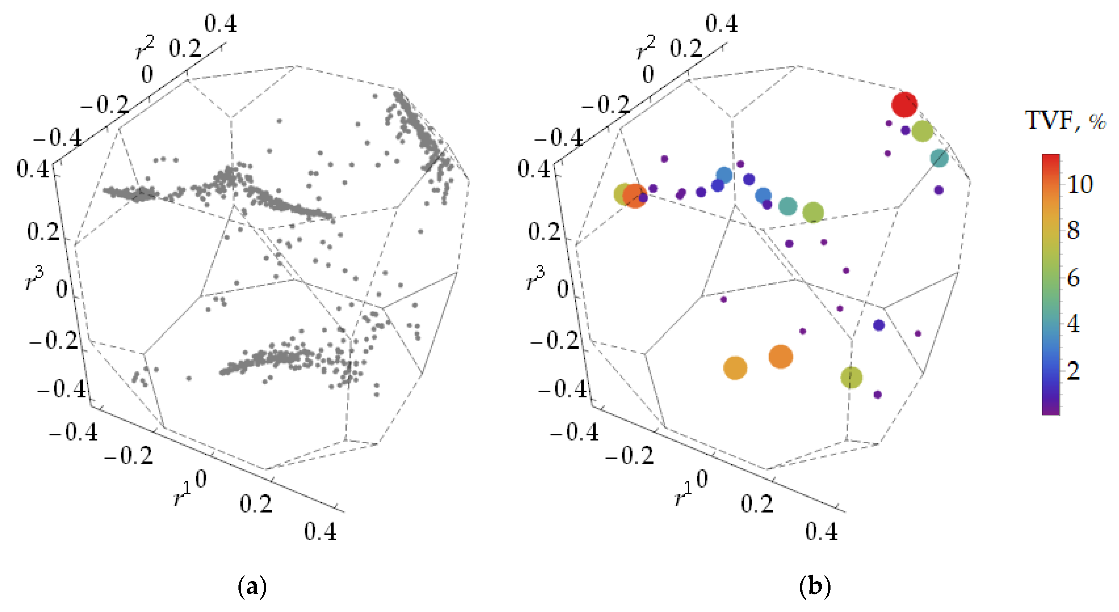
4. Some Numerical Results

The proposed CTC procedure was implemented (in the form of C++ libraries) and then applied to investigate some deformation textures simulated with the help of the multilevel crystal elasto–visco–plasticity model [63]. The verification of this model showed satisfactory agreement with experimental data. Results for two numerical tests are presented in this work. In each case, a PA of $N=1000$ copper (cubic symmetry) equal-volume crystallites after a kinematic loading along a trajectory with two active stages is considered. The first stages of both tests are described by the same velocity gradient tensor ${\mathbf{L}}^{\mathrm{I}}\in {\mathbb{E}}_3^{\left(2\right)}$:

$${\mathbf{L}}^{\mathrm{I}}=0.5\cdot {10}^{-3}\left(-l_1{l}_1+l_2{l}_2+l_1{l}_2-l_2{l}_1\right);$$

(32)

while the second ones are preceded by elastic unloadings (which do not affect the textures) and are determined by the different tensors ${\mathbf{L}}_1^{\mathrm{II}},{\mathbf{L}}_2^{\mathrm{II}}\in {\mathbb{E}}_3^{\left(2\right)}$:

$${\mathbf{L}}_1^{\mathrm{II}}=0.5\cdot {10}^{-3}\left(-l_1{l}_1+l_3{l}_3+l_1{l}_3-l_3{l}_1\right);$$

(33)

$${\mathbf{L}}_2^{\mathrm{II}}=0.5\cdot {10}^{-3}\left(-l_1{l}_1+l_2{l}_2-l_1{l}_2+l_2{l}_1\right).$$

(34)

Corresponding deformation paths are further referenced as Tests 1 and 2, respectively. Initial orientations of crystallites are chosen randomly with respect to the uniform distribution.

Obtained orientation distribution data sets are depicted in figures below by using the Rodrigues parametrization on ${\mathcal{O}}_{{\mathbb{S}}^{+}}^{+}$. This representation is obtainable with the help of the mapping $R:{\mathbb{O}}^{+}\to {\mathbb{E}}_3$ defined as

$$R\left[{\mathbf{R}}_a^{\alpha }\right]=\tan \frac{\alpha }{2}a.$$

(35)

The orientational space of interest is the image $R\left[{\mathcal{O}}_{{\mathbb{S}}^{+}}^{+}\right]$, which turns out to be a polyhedron for finite symmetry groups. Indeed, each ${\mathbf{R}}_u^{\omega }\in {\mathbb{S}}^{+}$ confines fundamental Rodrigues vectors to be between the following pair of planes (see Appendix B):

$$\pm r\cdot u=\tan \frac{\omega }{4},\hspace{1em}r\in R\left[{\mathbb{O}}^{+}\right].$$

(36)

Particularly, in the case of cubic symmetry, $R\left[{\mathcal{O}}_{{\mathbb{S}}^{+}}^{+}\right]$ is the truncated cube, faces of which are orthogonal to the $\langle 100\rangle$ and $\langle 111\rangle$ axes, and located at distances of $\sqrt{2}-1$ and $\sqrt{3}/3$ from the origin, respectively.

Figure 7a and Figure 8a show fundamental orientations of the textured PAs obtained in Tests 1 and 2. Their complete samples were processed using the CTC procedure with the following parameters (for both tests): $\omega =\epsilon =\delta /2=5°$; layer extractions were performed with values of $\phi$ chosen in the same way as for the exemplary sample considered in Section 4. The resulted reduced representations of the textures are given in Figure 7b and Figure 8b in the form of medoids weighted by the total volume fractions (TVFs) of crystallites with orientations in the corresponded clusters. Amounts of layers distinguished for Test 1 and 2 are 19 and 14, respectively. Orientations of the lowest layers, which appear to be isolated, are omitted in the figures (8.7% and 6% of the whole samples by the corresponding TVFs).

Diagrams for the instances of the CTC procedure showing the amount of clusters at the extracted layers versus the TVF of crystallites corresponded to orientations of these layers are provided in Figure 9. One can observe that for lower layers the amount of distinguished clusters increase dramatically as new layers are clustered. Thus, in order to achieve a good data reduction effect, it may be reasonable to restrict consideration to only few upper layers. Adequacy of representations emerging in such a way is discussed in Section 5.1. As a possible option for obtaining better data reduction, which seems to be especially relevant for weak textures, a subsample of statistically uniformly distributed orientations [54] can be preliminary filtered out (with the help of some auxiliary subprocedure) from a given sample. This subsample then can be effectively described by the TVF of corresponded crystallites and excluded from the sample in subsequent clustering.

5. Discussion

5.1. Adequacy Estimations

The crystallographic texture of a clustered PA can be represented reductively by using local approximations for orientation distribution in its clusters. One of the simplest examples of a reduced ODM, $F^{\mathrm{r}}$, in the notations of Section 3 is given by

$$F^{\mathrm{r}}={\displaystyle \sum _{l=1}^L{\displaystyle \sum _{k=1}^{K_l}\left({\displaystyle \sum _{n\in {\mathcal{C}}_{l\hspace{0.17em}k}}{f}_n}\right){\Delta }_{o_{m_{l\hspace{0.17em}k}}}}}.$$

(37)

In some cases, especially for wide clusters, more complicated variants may be used instead of the Dirac measures to approximate texture components. Various unimodal model functions are applicable for this purpose, e.g., those ones [35,36,37,38,39,40,41,46]. To estimate their parameters, statistical approaches can be employed. Note that a correct estimation expects orientations in each cluster to be the least deviated among their symmetric analogues from the corresponding medoid. Thus, some rearrangements in the sample of orientations are generally necessary:

$${\mathbf{o}}_n\leftarrow \underset{\mathbf{o}\in {\mathbb{S}}^{+}\cdot {\mathbf{o}}_n}{\arg \min }{d}_0\left[{\mathbf{o}}_{m_{l\hspace{0.17em}k}},\mathbf{o}\right],\hspace{1em}n\in {\mathcal{C}}_{l\hspace{0.17em}k},\hspace{1em}k\in \overline{1,K_l},\hspace{1em}l\in \overline{1,L}.$$

(38)

An important question here is the adequacy of such reduced representations. In practical applications, ODMs are usually required for aggregating various material properties. Let $F$ be the ODM of a single-phased polycrystalline RVE and ${\mathbf{\chi }}^{\#}\in {\mathbb{E}}_3^{\left(R\right)}$ ($R\in \left\{0,1,\dots \right\}$) be the tensor describing some characteristic of the crystalline lattice in its reference orientation. According to first-order homogenization theories, one can obtain an effective analogue, $\mathbf{{\rm X}}\in {\mathbb{E}}_3^{\left(R\right)}$, of this characteristic for the whole RVE by averaging:

$$\mathbf{{\rm X}}={\displaystyle \underset{\mathbf{o}\in {\mathbb{O}}^{+}}{\int }\mathbf{o}\ast {\mathbf{\chi }}^{\#}\mathrm{d}F}\left[\mathbf{o}\right].$$

(39)

The integrand in (39) corresponds to the property tensor of a crystalline lattice oriented by $\mathbf{o}$. The main thesis here is that every PA-induced ODM can be compared with its some reduced form in terms of, particularly, the differences in averaging certain material properties. In fact, such an approach introduces an external criterion of clustering quality.

For the textured PAs considered in Section 4, relative errors of representing ODMs in several reduced forms were evaluated from the viewpoint of elasticity. The results are described below within this subsection. Let ${\mathsf{\pi }}^{\#}\in {\mathbb{E}}_3^{\left(4\right)}$ be the elasticity tensor of the crystalline lattice in the reference position (with independent components being, in GPa, ${\pi }_{1111}^{\#}=168.4$, ${\pi }_{1122}^{\#}=121.4$, ${\pi }_{1212}^{\#}=75.4$ with respect to the corresponding basis). Aggregating this property by applying $F^{\mathrm{r}}$ as a ODM instead of $F$, leads to a change in the result, which can be estimated by the ratio [64]

$${\mathrm{RE}}^{\mathrm{r}}=\frac{{\overline{A}}^{\mathrm{r}}}{{\underset{\_}{\Pi }}^{\prime }}.$$

(40)

Herein, ${\underset{\_}{\Pi }}^{\prime }$ is the minimum non-zero eigenvalue of the unreduced effective elasticity tensor $\mathsf{П}$:

$$\mathsf{П}={\displaystyle \underset{\mathbf{o}\in {\mathbb{O}}^{+}}{\int }\mathbf{o}\ast {\mathsf{\pi }}^{\#}dF\left[\mathbf{o}\right]};$$

(41)

and ${\overline{A}}^{\mathrm{r}}$ is the maximum modulo eigenvalue of the residual tensor ${\mathbf{A}}^{\mathrm{r}}$ defined by

$${\mathbf{A}}^{\mathrm{r}}={\mathsf{П}}^{\mathrm{r}}-\mathsf{П},$$

(42)

where ${\mathsf{П}}^{\mathrm{r}}$ is the reduced effective elasticity tensor

$${\mathsf{П}}^{\mathrm{r}}={\displaystyle \underset{\mathbf{o}\in {\mathbb{O}}^{+}}{\int }\mathbf{o}\ast {\mathsf{\pi }}^{\#}d{F}^{\mathrm{r}}\left[\mathbf{o}\right]},$$

(43)

The designated eigenvalues are understood with respect to the problem of finding, for arbitrary $\mathbf{t}\in {\mathbb{E}}_3^{\left(4\right)}$, such $t\in ℂ$ and $\mathbf{s}\in {\mathbb{E}}_3^{\left(2\right)}\left(ℂ\right)$ that

$$\mathbf{t}:\mathbf{s}=t\mathbf{s}.$$

(44)

The value of (40) characterizes the maximum relative error which occurs in the stress tensor determined by the generalized Hooke’s law when $\mathsf{П}$ is approximated by ${\mathsf{П}}^{\mathrm{r}}$. Note that since the exact orientation distribution laws for the PAs are not known a priori (it is possible to only estimate them statistically), $F$ in the evaluations of $\mathsf{П}$ was set to the corresponding PA-induced ODMs.

Figure 10 shows dependencies of ${\mathrm{RE}}^{\mathrm{r}}$ for the mentioned PAs on the amount $\widehat{L}$ of upper sample layers considered as clustered ones. The contribution of such layers into each reduced ODM is adopted from (37), while the rest ones are treated by using the following three generally different approaches.

• Orientations of the rest layers are taken into consideration without any data reductions, i.e., just like in a PA-induced ODM. In such a way, these reduced ODMs arise:

  $$F_{1\hspace{0.17em}\widehat{L}}^{\mathrm{r}}={\displaystyle \sum _{l=1}^{\widehat{L}}{\displaystyle \sum _{k=1}^{K_l}\left({\displaystyle \sum _{n\in {\mathcal{C}}_{l\hspace{0.17em}k}}{f}_n}\right){\Delta }_{o_{m_{l\hspace{0.17em}k}}}}}+{\displaystyle \sum _{l=\widehat{L}+1}^L{\displaystyle \sum _{k=1}^{K_l}{\displaystyle \sum _{n\in {\mathcal{C}}_{l\hspace{0.17em}k}}{f}_n{\Delta }_{o_n}}}},\hspace{1em}\widehat{L}\in \overline{0,L}.$$

  (45)
• The rest layers are simply excluded from consideration. In this case, total volume fraction of crystallites corresponded to the remaining orientations requires renormalization so the reduced ODMs are:

  $$F_{2\hspace{0.17em}\widehat{L}}^{\mathrm{r}}=\frac{{\displaystyle \sum _{l=1}^{\widehat{L}}{\displaystyle \sum _{k=1}^{K_l}\left({\displaystyle \sum _{n\in {\mathcal{C}}_{l\hspace{0.17em}k}}{f}_n}\right){\Delta }_{o_{m_{l\hspace{0.17em}k}}}}}}{{\displaystyle \sum _{l=1}^{\widehat{L}}{\displaystyle \sum _{k=1}^{K_l}{\displaystyle \sum _{n\in {\mathcal{C}}_{l\hspace{0.17em}k}}{f}_n}}}},\hspace{1em}\widehat{L}\in \overline{1,L}.$$

  (46)
• Orientations of the rest layers are taken as uniformly distributed ones providing the following reduced ODMs:

  $$F_{3\hspace{0.17em}\widehat{L}}^{\mathrm{r}}={\displaystyle \sum _{l=1}^{\widehat{L}}{\displaystyle \sum _{k=1}^{K_l}\left({\displaystyle \sum _{n\in {\mathcal{C}}_{l\hspace{0.17em}k}}{f}_n}\right){\Delta }_{o_{m_{l\hspace{0.17em}k}}}}}+\left({\displaystyle \sum _{l=\widehat{L}+1}^L{\displaystyle \sum _{k=1}^{K_l}{\displaystyle \sum _{n\in {\mathcal{C}}_{l\hspace{0.17em}k}}{f}_n}}}\right)U,\hspace{1em}\widehat{L}\in \overline{0,L}.$$

  (47)

Since the reduced-form ODMs listed above are identical to each other when $\widehat{L}=L$, the shown plots meet at the corresponding points. It is observed that texture representations given by (47) turn out to be more accurate (with respect to aggregating elastic characteristics) than ones for (46) while their data reduction effects are almost the same.

5.2. An Application to Approximating Orientation Distribution Functions for Generating Textured Polycrystalline Aggregates

Peak-type texture components identified by the CTC procedure and approximated with the help of some model functions provide an estimated ODF, which can be used for generating correspondingly textured PAs. Particularly, such a task is of interest in numerical investigations (on the basis of statistical multilevel polycrystalline models) of processes related to thermo–mechanical treatment of initially textured materials. In this subsection, comparison between the PAs considered in the above examples and random PAs generated with respect to the estimated ODFs is performed.

The generating ODFs were chosen to be of the form

$$f_{\widehat{L}}^{\mathrm{r}}\left[\mathbf{o}\right]={\displaystyle \sum _{l=1}^{\widehat{L}}{\displaystyle \sum _{k=1}^{K_l}\left({\displaystyle \sum _{n\in {\mathcal{C}}_{l\hspace{0.17em}k}}{f}_n}\right)\frac{\exp \left[{\kappa }_{l\hspace{0.17em}k}\cos d\left[{\mathbf{o}}_{m_{l\hspace{0.17em}k}},\mathbf{o}\right]\right]}{I_0\left[{\kappa }_{l\hspace{0.17em}k}\right]-I_1\left[{\kappa }_{l\hspace{0.17em}k}\right]}}}+\left({\displaystyle \sum _{l=\widehat{L}+1}^L{\displaystyle \sum _{k=1}^{K_l}{\displaystyle \sum _{n\in {\mathcal{C}}_{l\hspace{0.17em}k}}{f}_n}}}\right),\hspace{1em}\widehat{L}\in \overline{0,L-1},$$

(48)

where ${\kappa }_{1\hspace{0.17em}1},\dots ,{\kappa }_{L-1\hspace{0.17em}{K}_{L-1}}\ge 0$ are scatter parameters estimated independently in each cluster by the maximum log-likelihood method and $I_n$ is the $n$-th modified Bessel function. The left term of (48) corresponds, if (38) is applied, to a special case of the von Mises–Fisher distribution [53], while the right term contributes with uniformly distributed orientations. Such ODFs can be easily identified since all necessary pseudometric distance statistics are obtainable directly from the CTC procedure. Just like in (45)–(47), $\widehat{L}$ specifies the amount of layers taken as clustered ones.

An artificially generated PA of $N^{\mathrm{g}}$ crystallites with orientations ${\mathbf{o}}_1^{\mathrm{g}},\dots ,{\mathbf{o}}_{N^{\mathrm{g}}}^{\mathrm{g}}\in {\mathbb{O}}^{+}$ and equal (for simplicity) volume fractions can be compared with a given PA in terms of elastic properties aggregated with their induced ODMs. Herein, the difference in the aggregation results is estimated by

$${\mathrm{RE}}^{\mathrm{g}}=\frac{{\overline{A}}^{\mathrm{g}}}{{\underset{\_}{\Pi }}^{\prime }},$$

(49)

where ${\overline{A}}^{\mathrm{g}}$ is the maximum modulo eigenvalue of the residual tensor ${\mathbf{A}}^{\mathrm{g}}$ defined by

$${\mathbf{A}}^{\mathrm{g}}={\displaystyle \underset{\mathbf{o}\in {\mathbb{O}}^{+}}{\int }\mathbf{o}\ast {\mathsf{\pi }}^{\#}d{F}^{\mathrm{g}}\left[\mathbf{o}\right]}-\mathsf{П},$$

(50)

and $F^{\mathrm{g}}$ is the ODM induced by the generated PA:

$$F^{\mathrm{g}}=\frac{1}{N^{\mathrm{g}}}{\displaystyle \sum _{n=1}^{N^{\mathrm{g}}}{\Delta }_{{\mathbf{o}}_n^{\mathrm{g}}}}.$$

(51)

For both PAs given in the examples, 20 random realizations of PAs with $N^{\mathrm{g}}=N=1000$ crystallites were constructed for each admissible $\widehat{L}$ by using $f_{\widehat{L}}^{\mathrm{r}}$ for sampling orientations. Obtained values of ${\mathrm{RE}}^{\mathrm{g}}$ are plotted below in Figure 11.

One can notice that the dependencies established for the mean values of ${\mathrm{RE}}^{\mathrm{g}}$ provide statistical estimates for the adequacy of the reduced texture representations given by (48). Such representations are similar to (47), but rely on certain continuous local approximations of texture components instead of simple medoid-concentrated ones. It appears, however, that the applied approximating functions do not improve accuracy. Such a circumstance is due to the independence these functions on axes of rotations to their maximum points. Thus, morphology of obtained clusters is not taken into consideration, as it can be observed from Figure 12, where corresponding typical samples of random orientations are depicted for $\widehat{L}=L-1$. In order to eliminate this feature, one can employ the anisotropic component functions [39,53]. Nonetheless, from the viewpoint of aggregating elastic properties, generated PAs turn out to be satisfactory close to the given ones.

6. Conclusions

To sum up, the problem of reducing orientation distribution data for a textured polycrystalline aggregate in considered within this paper. In order to perform such a reduction, an approach based on identifying statistically preferred crystalline orientations in a given fraction-weighted (by volumes of corresponded crystallites) sample is proposed. The procedure developed for executing this task is described in details. Its algorithm includes several logically separate stages, which divide the sample into distinct subsets of close orientations with the help of various techniques of Cluster Analysis. These stages, briefly characterized as “layer extracting”, “pre-clustering”, and “post-clustering”, complement each other providing heuristically sensible partitions at different distribution density levels. The mentioned concept of closeness between orientations is introduced with lattice symmetry of crystallites taken into consideration. For this purpose, the special comparison function equal to the minimal rotation angle between symmetrical equivalents of argument orientations is defined. It turns out that such a function corresponds to a symmetry-invariant pseudometric distance induced by the natural Riemann metrics. Since all algorithms formulated in the work operate with orientations belonging exclusively to the sample, it is reasonable to pre-compute and tabulate the distances between them, obtaining thereby the so-called misorientation matrix.

The results of applying the developed clustering procedure to reducing two numerically simulated (in deformation tests) crystallographic textures are given for demonstration purposes. Three approaches to define a reduced-form orientation distribution measure are considered and juxtaposed with each other in terms of aggregating elastic characteristics. It is observed that clustering-based texture representations are able to provide adequate responses using a relatively small (compared to the amount of crystallites in the aggregates) amount of clusters. In addition, local orientation distributions within each obtained cluster are estimated statistically in the form of the von Mises–Fisher distribution by employing the maximum log-likelihood method. Distributions estimated in such a way can be used in generating correspondingly textured polycrystalline aggregates for various applications. Comparisons between the given and generated aggregates are performed analogically to the case of juxtaposing with reduced representations.

In the problems related to the design of functional polycrystalline materials, a great amount of degrees of freedom is a common issue. The proposed clustering procedure seems to be useful in this regard. With its help, typical most intensive texture components can be identified in certain classes of thermo–mechanical treatment processes. Such components provide a reduced basis for searching orientation distributions and appropriate treatment regimens resulting in better performance of a material product.

References

1. Taylor, G.I.; Elam, C.F. The distortion of an aluminium crystal during a tensile test. Proc. Roy. Soc. Ser. A 1923, 102, 643–647. [Google Scholar]
2. Taylor, G.I.; Elam, C.F. The plastic extension and fracture of aluminium crystals. Proc. Roy. Soc. Ser. A 1925, 108, 28–51. [Google Scholar]
3. Sachs, G.O. Zur Ableitungeiner Fliessbedingung. Z. Ver. Deut. Ing. 1928, 72, 734–736. [Google Scholar]
4. Masimo, M.; Sachs, G.O. Mechanische Eigenschaften von Messingkristallen. Z. Phys. 1928, 50, 161–186. [Google Scholar] [CrossRef]
5. Taylor, G.I. Plastic strain in metals. J. Inst. Met. 1938, 62, 307–324. [Google Scholar]
6. Bishop, J.F.W.; Hill, R. A theory of the plastic distortion of a polycrystalline aggregate under combined stresses. Phil. Mag. Ser. 7 1951, 42, 414–427. [Google Scholar] [CrossRef]
7. Bishop, J.F.W.; Hill, R. A theoretical derivation of the plastic properties of a polycrystalline face-centred metal. Phil. Mag. Ser. 7 1951, 42, 1298–1307. [Google Scholar] [CrossRef]
8. Lin, T.H. Analysis of elastic and plastic strains of a face-centered cubic crystal. J. Mech. Phys. Solids 1957, 5, 143–149. [Google Scholar] [CrossRef]
9. Anand, L. Single-crystal elasto-viscoplasticity: Application to texture evolution in polycrystalline metals at large strains. Comput. Methods Appl. Mech. Eng. 2004, 193, 5359–5383. [Google Scholar] [CrossRef]
10. McDowell, D.L.; Olson, G.B. Concurrent design of hierarchical materials and structures. In Lecture Notes in Computational Science and Engineering; Springer: Berlin/Heidelberg, Germany, 2008; Volume 68, pp. 207–240. ISBN 9781402097409. [Google Scholar]
11. Van Houtte, P. Crystal plasticity based modelling of deformation textures. In Microstructure and Texture in Steels; Haldar, A., Suwas, S., Bhattacharjee, D., Eds.; Springer: Berlin/Heidelberg, Germany, 2009; pp. 209–224. ISBN 978-1-84882-454-6. [Google Scholar]
12. Roters, F.; Eisenlohr, P.; Hantcherli, L.; Tjahjanto, D.D.; Bieler, T.R.; Raabe, D. Overview of constitutive laws, kinematics, homogenization and multiscale methods in crystal plasticity finite-element modeling: Theory, experiments, applications. Acta Mater. 2010, 58, 1152–1211. [Google Scholar] [CrossRef]
13. Trusov, P.V.; Shveykin, A.I. Multilevel crystal plasticity models of single- and polycrystals. Statistical Models. Phys. Mesomech. 2013, 16, 23–33. [Google Scholar] [CrossRef]
14. Trusov, P.V.; Shveykin, A.I. Multilevel crystal plasticity models of single- and polycrystals. Direct models. Phys. Mesomech. 2013, 16, 99–124. [Google Scholar] [CrossRef]
15. Trusov, P.V.; Shveykin, A.I. Multilevel Models of Mono- and Polycrystalline Materials: Theory, Algorithms, Application Examples; SO RAN: Novosibirsk, Russia, 2019; ISBN 978-5-7692-1661-9. [Google Scholar]
16. Busso, E.P. Multiscale Approaches: From the Nanomechanics to the Micromechanics. In Computational and Experimental Mechanics of Advanced Materials; Silberschmidt, V.V., Ed.; Springer: Berlin/Heidelberg, Germany, 2006; pp. 141–165. [Google Scholar]
17. Luscher, D.J.; McDowell, D.L. An extended multiscale principle of virtual velocities approach for evolving microstructure. Procedia Eng. 2009, 1, 117–121. [Google Scholar] [CrossRef] [Green Version]
18. Luscher, D.J.; McDowell, D.L.; Bronkhorst, C.A. A second gradient theoretical framework for hierarchical multiscale modeling of materials. Int. J. Plast. 2010, 26, 1248–1275. [Google Scholar] [CrossRef]
19. Clement, A. Prediction of deformation texture using a physical principle of conservatiol. Mater. Sci. Eng. 1982, 55, 203–210. [Google Scholar] [CrossRef]
20. Kumar, A.; Dawson, P.R. The simulation of texture evolution with finite elements over orientation space II. Application to planar crystals. Comput. Methods Appl. Mech. Eng. 1996, 130, 247–261. [Google Scholar] [CrossRef]
21. Kumar, A.; Dawson, P.R. The simulation of texture evolution with finite elements over orientation space I. Development. Comput. Methods Appl. Mech. Eng. 1996, 130, 227–246. [Google Scholar] [CrossRef]
22. Kumar, A.; Dawson, P.R. Modeling crystallographic texture evolution with finite elements over neo-Eulerian orientation spaces. Comput. Methods Appl. Mech. Eng. 1998, 153, 259–302. [Google Scholar] [CrossRef]
23. Acharjee, S.; Zabaras, N. A proper orthogonal decomposition approach to microstructure model reduction in Rodrigues space with applications to optimal control of microstructure-sensitive properties. Acta Mater. 2003, 51, 5627–5646. [Google Scholar] [CrossRef]
24. Ganapathysubramanian, S.; Zabaras, N. Modeling the thermoelastic-viscoplastic response of polycrystals using a continuum representation over the orientation space. Int. J. Plast. 2005, 21, 119–144. [Google Scholar] [CrossRef]
25. Lebensohn, R.A. N-site modeling of a 3D viscoplastic polycrystal using Fast Fourier Transform. Acta Mater. 2001, 49, 2723–2737. [Google Scholar] [CrossRef]
26. Hu, L.; Rollet, A.D.; Iadicola, M.; Foecke, T.; Banovic, S. Constitutive Relations for AA 5754 Based on Crystal Plasticity. Met. Mater. Trans. A 2012, 43, 854–869. [Google Scholar] [CrossRef]
27. Bunge, H.-J. Texture Analysis in Materials Science. Mathematical Methods; Elsevier Ltd.: Amsterdam, The Netherlands, 1969; ISBN 978-0-408-10642-9. [Google Scholar]
28. Sam, D.; Onat, E.; Etingof, P.; Adams, B. Coordinate free tensorial representation of the orientation distribution function with harmonic polynomials. Textures Microstruct. 1993, 21, 233–250. [Google Scholar] [CrossRef] [Green Version]
29. Ganapathysubramanian, S.; Zabaras, N. Design across length scales: A reduced-order model of polycrystal plasticity for the control of microstructure-sensitive material properties. Comput. Methods Appl. Mech. Eng. 2004, 193, 5017–5034. [Google Scholar] [CrossRef]
30. Sundararaghavan, V.; Zabaras, N. On the synergy between texture classification and deformation process sequence selection for the control of texture-dependent properties. Acta Mater. 2005, 53, 1015–1027. [Google Scholar] [CrossRef]
31. Holmes, P.; Lumley, J.L.; Berkooz, G.; Rowley, C.W. Proper orthogonal decomposition. In Turbulence, Coherent Structures, Dynamical Systems and Symmetry; Cambridge University Press: Cambridge, UK, 2012; pp. 68–105. [Google Scholar]
32. Sirovich, L. Turbulence and the dynamics of coherent structures. I. Coherent structures. Qarterly Appl. Math. 1987, 45, 561–571. [Google Scholar] [CrossRef] [Green Version]
33. Ruer, D.; Baro, R. Vectorial method of texture analysis of cubic lattice polycrystalline material. J. Appl. Cryst. 1977, 10, 458–464. [Google Scholar] [CrossRef]
34. Matthies, S. The ODF-Spectrum a New and Comprehensive Characterization of the Degree of Anisotropy of Orientation Distributions. Mater. Sci. Forum 2005, 495–497, 331–338. [Google Scholar] [CrossRef]
35. Matthies, S. Form effects in the description of the orientation distribution function (ODF) of texturized materials by model components. Phys. Status Solidi 1982, 112, 705–716. [Google Scholar] [CrossRef]
36. Luecke, K.; Jura, J.; Pospiech, J.; Hirsch, J.R. On the presentation of orientation distribution functions by model functions. Z. Met. 1986, 77, 312–321. [Google Scholar]
37. Helming, K.; Eschner, T. A new approach to texture analysis of multiphase materials using a texture component model. Cryst. Res. Technol. 1990, 25, 203–208. [Google Scholar] [CrossRef]
38. Helming, K.; Schwarzer, R.A.; Rauschenbach, B.; Geier, S.; Leiss, B.; Heinitz, J. Texture estimates by means of components. Z. Met. 1994, 85, 545–553. [Google Scholar]
39. Eschner, T.; Fundenberger, J.-J. Application of anisotropic texture components. Textures Microstruct. 1997, 28, 181–195. [Google Scholar] [CrossRef] [Green Version]
40. Raabe, D.; Roters, F. Using texture components in crystal plasticity finite element simulations. Int. J. Plast. 2004, 20, 339–361. [Google Scholar] [CrossRef]
41. Ivanova, T.M.; Savyolova, T.I.; Sypchenko, M.V. The modified component method for calculation of orientation distribution function from pole figures. Inverse Probl. Sci. Eng. 2010, 18, 163–171. [Google Scholar] [CrossRef]
42. Chateigner, D. Quantitative Texture Analysis. In Combined Analysis; ISTE Ltd.: London, UK, 2013; pp. 95–190. ISBN 9781118622506. [Google Scholar]
43. Suwas, S.; Ray, R.K. Crystallographic Texture of Materials; Springer: London, UK, 2014; ISBN 978-1-4471-6314-5. [Google Scholar]
44. Mokrova, S.M.; Petrov, R.P.; Milich, V.N. Determination of the texture of polycrystalline materials using an algorithm of object-vector representation of reflection planes and visualization of the results in Rodrigues space. Vestn. Udmurt. Univ. Mat. Mekh. Komp. Nauk. 2016, 26, 336–344. [Google Scholar] [CrossRef] [Green Version]
45. Ostapovich, K.V.; Trusov, P.V.; Yanz, A.Y. An algorithm for identifying texture components in the framework of statistical crystal plasticity models. IOP Conf. Ser. Mater. Sci. Eng. 2019, 581, 12014. [Google Scholar] [CrossRef]
46. Ostapovich, K.V.; Trusov, P.V. Investigation of crystallographic textures in multi-level models for polycrystalline deformation using clustering techniques. Comput. Contin. Mech. 2019, 12, 67–79. [Google Scholar] [CrossRef] [Green Version]
47. Ostapovich, K.V.; Trusov, P.V. An application of clustering techniques to reducing crystallographic texture data. AIP Conf. Proc. 2020, 2216, 70003. [Google Scholar]
48. Trusov, P.V.; Dudar’, O.I.; Keller, I.E. Tensor Algebra and Analysis; Perm State Technical University: Perm, Russia, 1998; ISBN 5-88151-148-4. [Google Scholar]
49. Bertram, A. Mathematical Preparation. In Elasticity and Plasticity of Large Deformations: An Introduction; Springer: Berlin/Heidelberg, Germany, 2012; pp. 3–90. ISBN 978-3-642-24615-9. [Google Scholar]
50. Weyl, H. The Classical Groups: Their Invariants and Representations, 2nd ed.; Princeton University Press: Princeton, NJ, USA, 1966; ISBN 9780691057569. [Google Scholar]
51. Halmos, P.R. Measure Theory; Springer: New York, NY, USA, 1974. [Google Scholar]
52. Reed, M.; Simon, B. Methods of Modern Mathematical Physics. I: Functional Analysis, 1st ed.; Academic Press: Cambridge, MA, USA, 1980; ISBN 978-0157850505. [Google Scholar]
53. Morawiec, A. Orientations and Rotations; Springer: Berlin/Heidelberg, Germany, 2004; ISBN 978-3-662-09156-2. [Google Scholar]
54. Arnold, R.; Jupp, P.E.; Schaeben, H. Statistics of ambiguous rotations. J. Multivar. Anal. 2017, 165, 73–85. [Google Scholar] [CrossRef] [Green Version]
55. Altmann, S.L. Rotations, Quaternions, and Double Groups; Dover Publications: Mineola, NY, USA, 2013; ISBN 9780486317731. [Google Scholar]
56. Heinz, A.; Neumann, P. Representation of Orientation and Disorientation Data for Cubic, Hexagonal, Tetragonal and Orthorhombic Crystals. Acta Cryst. 1991, A47, 780–789. [Google Scholar] [CrossRef]
57. Pospiech, J. Die Parameter der Drehung und die Orientierungsverteilungsfunktion (OVF). Kristall und Technik 1972, 7, 1057–1072. [Google Scholar] [CrossRef]
58. Hastie, T.; Tibshirani, R.; Friedman, J. The Elements of Statistical Learning: Data Mining, Inference, and Prediction, 2nd ed.; Springer: New York, NY, USA, 2009; ISBN 9780387848570. [Google Scholar]
59. Kriegel, H.-P.; Kröger, P.; Jörg, S.; Arthur, Z. Density-based clustering. Wiley Interdiscip. Rev. Data Min. Knowl. Discov. 2011, 1, 231–240. [Google Scholar] [CrossRef]
60. Ester, M.; Kriegel, H.-P.; Jörg, S.; Xu, X. A density-based algorithm for discovering clusters in large spatial databases with noise. In Proceedings of the 2nd ACM International Conference on Knowledge Discovery and Data Mining (KDD), Portland, Oregon, 2–4 August 1996; pp. 226–231. [Google Scholar]
61. Kaufman, L.; Rousseeuw, P. Finding Groups in Data: An Introduction to Cluster Analysis; John Wiley & Sons: Hoboken, NJ, USA, 1990; ISBN 0-471-73578-7. [Google Scholar]
62. Massart, D.L.; Plastria, F.; Kaufman, L. Non-hierarchical clustering with MASLOC. Pattern Recognit. 1983, 16, 507–516. [Google Scholar] [CrossRef]
63. Trusov, P.V.; Shveykin, A.I. Motion decomposition, frame-indifferent derivatives, and constitutive relations at large displacement gradients from the viewpoint of multilevel modeling. Phys. Mesomech. 2017, 20, 357–376. [Google Scholar] [CrossRef]
64. Trusov, P.V.; Ostapovich, K.V. On Elastic Symmetry Identification for Polycrystalline Materials. Symmetry 2017, 9, 240. [Google Scholar] [CrossRef] [Green Version]
65. Park, F.C. Distance metrics on the rigid-body motions with applications to mechanism design. ASME J. Mech. Des. 1995, 117, 48–54. [Google Scholar] [CrossRef]
66. Park, F.C.; Ravani, B. Smooth invariant interpolation of rotations. ACM Trans. Graph. 1997, 16, 277–295. [Google Scholar] [CrossRef]
67. Huynh, D.Q. Metrics for 3D Rotations: Comparison and Analysis. J. Math. Imaging Vis. 2009, 155–164. [Google Scholar] [CrossRef]
Figure 1. Orientations of the exemplary sample. Each vertical line indicates an orientation angle.
Crystals 11 00336 g001
Figure 2. Weights calculated for the exemplary sample.
Crystals 11 00336 g002
Figure 3. A layer extracted from the exemplary sample by Algorithm 1.
Crystals 11 00336 g003
Figure 4. Clusters obtained by Algorithm 2 for the extracted layer. Orientations with angles near 0 and π are close to each to other due to the given symmetry.
Crystals 11 00336 g004
Figure 5. Refined clusters and medoids obtained by Algorithm 3 for the pre-clustered layer: (a) before splitting; (b) after splitting and subsequent medoid-based reclustering.
Crystals 11 00336 g005
Figure 6. The scheme of transitions between main operations in Algorithm 4.
Crystals 11 00336 g006
Figure 7. (a) The crystallographic texture formed in Test 1 and (b) its medoid-based reduced representation.
Crystals 11 00336 g007
Figure 8. (a) The crystallographic texture formed in Test 2 and (b) its medoid-based reduced representation.
Crystals 11 00336 g008
Figure 9. The amount of clusters distinguished during the crystallographic texture clustering (CTC) procedure for polycrystalline aggregates (PAs) obtained in Tests (a) 1 and (b) 2. Each plot point corresponds to an end of the post-clustering stage.
Crystals 11 00336 g009
Figure 10. The estimates of relative errors in aggregating elastic characteristics caused by using different reduced orientation distribution measures (ODMs) for the PAs obtained in Tests (a) 1 and (b) 2.
Crystals 11 00336 g010
Figure 11. The estimated differences of elastic characteristics averaged over PAs obtained in Tests (a) 1 and 2 (b) with the ones averaged over random PAs generated by using different approximating ODFs. Mean values are computed by averaging over realizations corresponding to the same ODFs.
Crystals 11 00336 g011
Figure 12. Typical random samples of orientations generated with respect to the ODFs estimated by PAs obtained in Tests (a) 1 and 2 (b).
Crystals 11 00336 g012
Publisher’s Note: MDPI stays neutral with regard to jurisdictional claims in published maps and institutional affiliations.