The current work became true during our numerical investigation of the deformation behavior of polycrystalline Ag/SnO
2 oxide dispersion strengthened (ODS) MMCs. Experimental results can be referred to Wasserbäch et al. [
14,
15]. For FE simulations, micromechanical features need to be considered, like the local interaction among Ag-Ag grains and Ag-SnO
2 (grain-particle), the Ag grain orientation, the particle size and distribution, as well as the microstructure representativeness. It is well known that the particle phase volume fraction on the microscale is very influential to the homogenized macroscopic
behavior. If such an FE simulation should predict the deformation behavior in detail, the volume fraction of the strengthening phase should be firstly guaranteed, i.e., the particle volume fraction in the simulation should be approximately the same as the real one.
2.1. Insensibility of Phase Volume Ratios to Microstructure Position in Axisymmetric FE Analyses
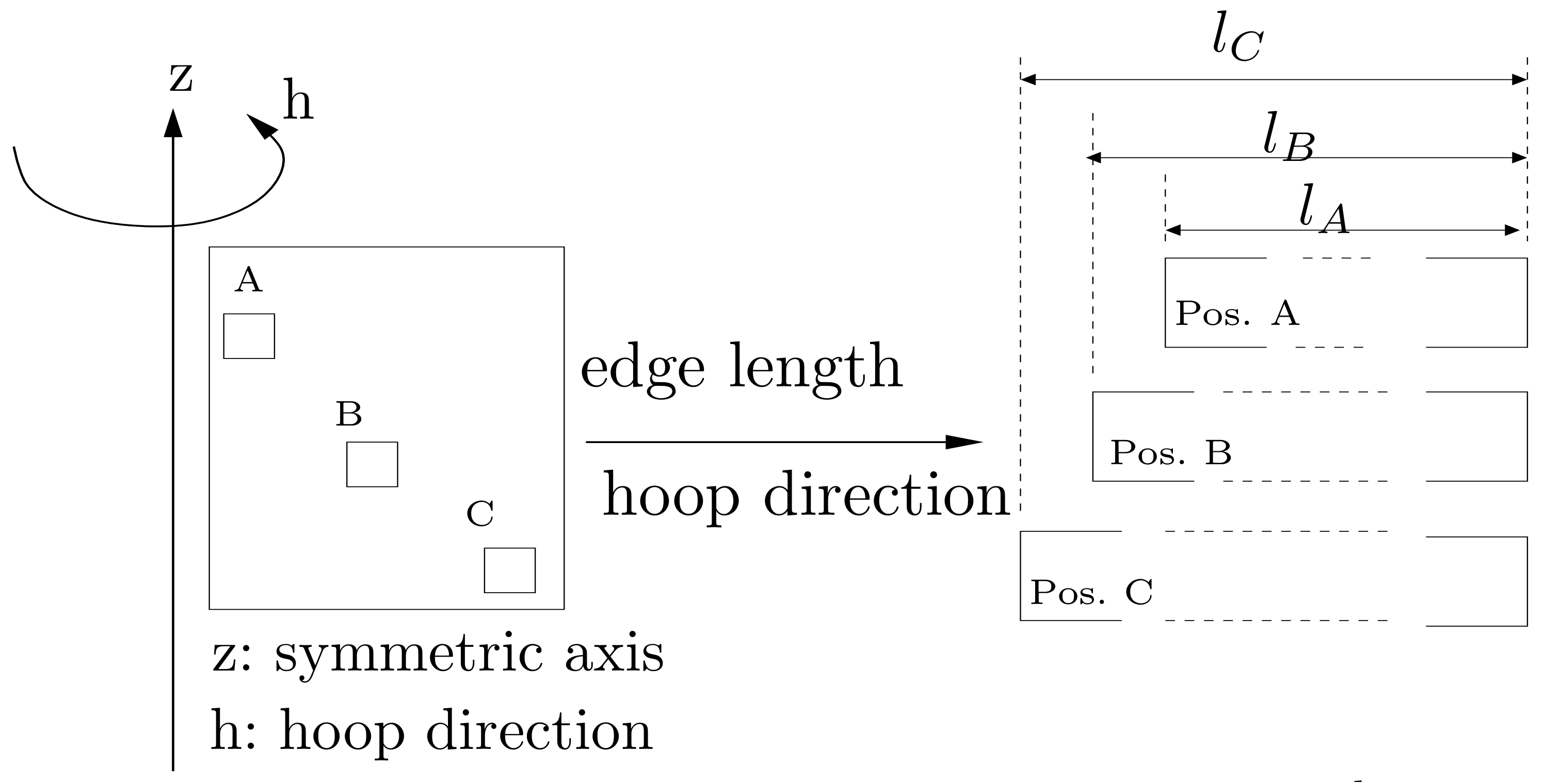
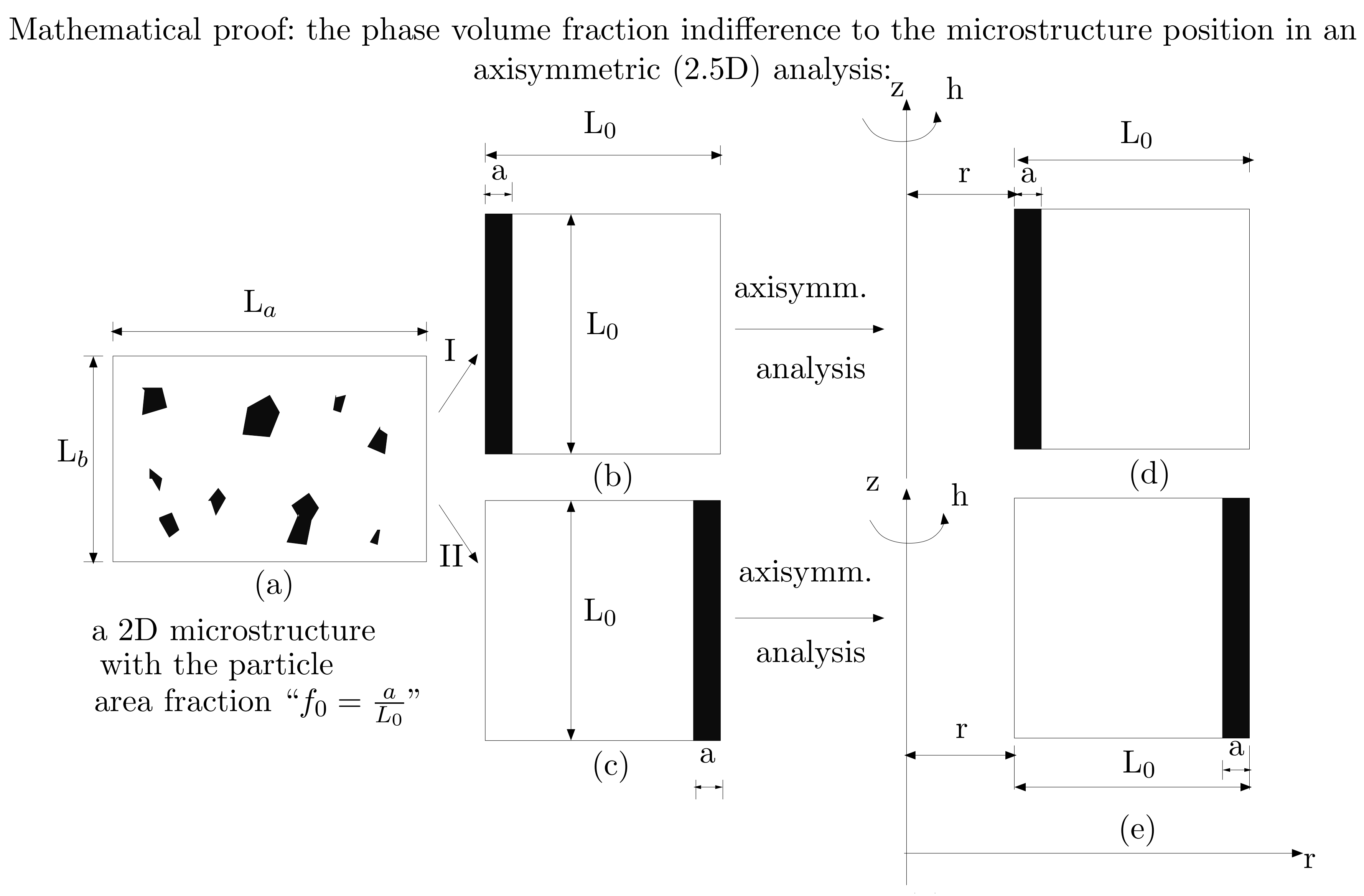
Besides 2D and 3D FE simulations (ABAQUS), the axisymmetry (2.5D) is also an analysis type. To be clear, the real structure geometry in an axisymmetric simulation is not necessarily axisymmetric. Another point is that the coordinate system in an axisymmetric (2.5D) analysis can be the same as the one in a 3D analysis. The geometrical assumption in a 2D analysis is infinite in the third direction. In an axisymmetric analysis, this assumption is finite (
Figure 1). Concerning this geometric assumption in the third direction, the axisymmetric analysis (2.5D) has an improvement compared to the 2D one. Micromechanical axisymmetric (2.5D) simulations possess several advantages: (I) such “2.5D” simulations are as time efficient as 2D simulations. (II) A full presentation of a variable in all the three directions can be realized in an axisymmetric (2.5D) simulation, but not in a 2D simulation. (III) Especially, it is useful for simulations with a user sub-routine “UMAT” (ABAQUS), since only one “UMAT” is enough for both the axisymmetric (2.5D) and the 3D simulations. Generally, a “UMAT” developed for the 3D case cannot be applied in 2D simulations. (IV) Furthermore, a meshed 2D structure can be directly used in an axisymmetric simulation by simply changing element types into “CAX” element type (ABAQUS). Even though 3D FE analyses generally yield better predicted results than 2D and axisymmetric ones, 3D simulations are often limited by the calculation capacity, since the total number of elements is easily exceeding the FE calculation limit. For a 3D geometrical adaptive meshing, the phase volume fraction calculated from elements can show a large discrepancy compared to the one calculated by pixels. Still, no concrete relation exists between the phase volume fraction (from elements) after meshing and the one before meshing (from pixels), i.e., this problem is not easy to be under user-control. This volume deviation becomes more serious for fine particle strengthened materials and the difference can be around 10% and even higher. Comparatively, from our experience, the aforementioned discrepancy is less than 1% for 2D (axisymmetry) analyses. Besides the analysis types, there are other important factors influencing the accuracy of FE results, like used theories, boundary conditions (BCs) and whether statistical data is large enough. Considering advantages and disadvantages of the three analyzing types, no one can completely replace another, i.e., further coexistence.
To investigate the deformation behavior and the texture evolution of the Ag/SnO
2 ODS, the elasto-visco-plastic material model, including the crystal plasticity theory, is applied for polycrystalline Ag grains on the microscopic level. This is realized for the simulation in the form of the user sub-routine “UMAT”. The user sub-routine was developed at the Institute of Mechanics of Otto-von-Guericke-University Magdeburg, Germany. In the past, it was already applied for various materials under different loading cases [
7,
16,
17,
18,
19,
20,
21,
22,
23,
24,
25].
Section 2.1.1 presents a short description of the applied material model.
For our axisymmetric (2.5D) two-scale FE simulations, the Ag:SnO
2 volume ratio in the microstructure should be the same as the real one (Ag:SnO
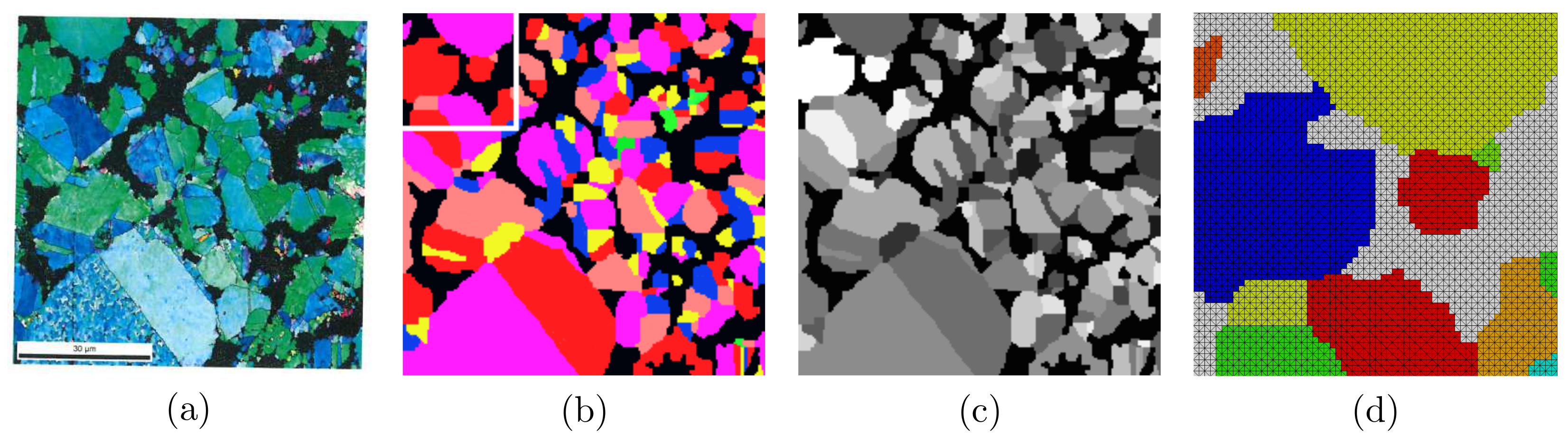
2 = 83 vol.%:17 vol.%). Here, the “same” ratio means within a tolerable difference, e.g., within 1–2 vol.%. Our applied microstructures are obtained from EBSD tests. Such images have an original resolution of
pixels and dimensions of
μm
2. The particle phase is presented in black, e.g.,
Figure 2a. The SnO
2 phase is 24 vol.% (24% area fraction) in
Figure 2a. In the current work, “vol.%” symbol is also valid for the area fraction in 2D cases, since it is convenient to compare 3D phase volume ratios with 2D phase area ratios. The hard particle volume fraction is 7 vol.% higher in the microstructure than in the real one. It is outside of the tolerable range. In order to obtain the real composition, the first step (method) is to find a suitable position for the microstructure in the macro cross section. This method is called “numerical volume searching” in the current work, i.e., finding a suitable position for the microstructure in the macro cross section so that a desired phase volume ratio can be reached. Since the element volume (“EVOL” in ABAQUS) is position dependent.
Figure 1 schematically presents this position dependence of the element volume. To be more precise, the volume is position dependent in “r” direction (
Figure 3b), if the area of an element (“CAX” element type) is fixed. The numerical search for the aforementioned suitable position is done in 3 steps: (I) the picture handling based on pixels; (II) the selection of a desired size, and (III) the numerical calculation of phase volume ratios. More in detail:
(I) The pixel handling is done for a real microstructure of the Ag/17 vol.%SnO
2 ODS (
Figure 2a).
Figure 2b is the resulting image. In
Figure 2b, there are 171 colored Ag grains, and the SnO
2 phase is given in black. For simplicity, the American standard code for information interchange (ASCII) format of images in a grey scale (
Figure 2c) is preferred in further steps, since data in this format are convenient for illustration and data processing. In
Figure 2c, the color of each pixel is described by only one integer in the range of [0, 255], i.e., one channel.
(II) As an example, a small cut-out of the microstructure shown in the upper left corner of
Figure 2b (also see
Figure 3a) is selected in search of a desired position, at which the phase volume ratio is Ag:SnO
2 = 83 vol.%:17 vol.%. This small cut-out corresponds to about
μm
2 and has about 25.5% area fraction of the SnO
2 phase. There are totally 11 Ag grains.
(III) A code is developed to find a suitable position for the microstructure in the macro cross section. At this suitable position, the volume fraction of the inclusion phase should approximately match the real one. In our example, it is 17 vol.% for the SnO2 phase.
Our samples have a diameter of 5 mm after two passes of hot extrusions. The ones before the extrusion have a diameter of 85 mm, i.e., the chamber for the extrusion has a diameter of 85 mm.
Figure 2a corresponds to a material status before extrusion. It means that
Figure 2a is a cut-out from a green body.
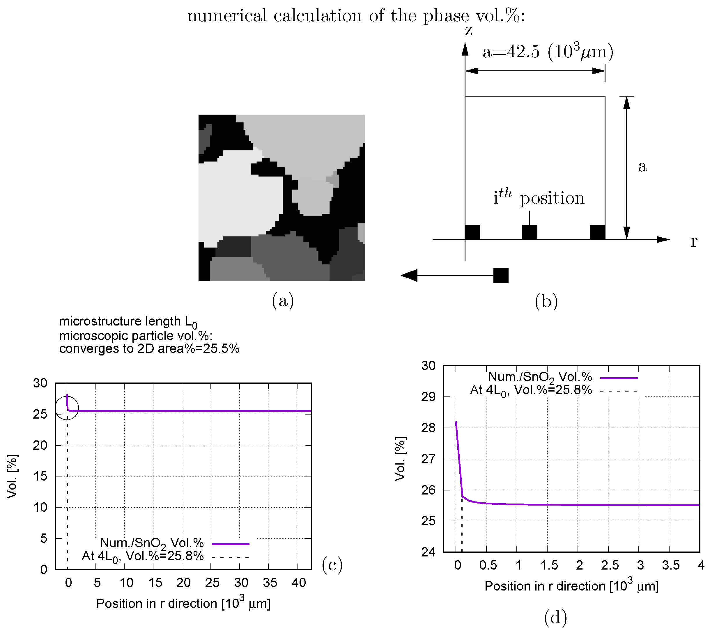
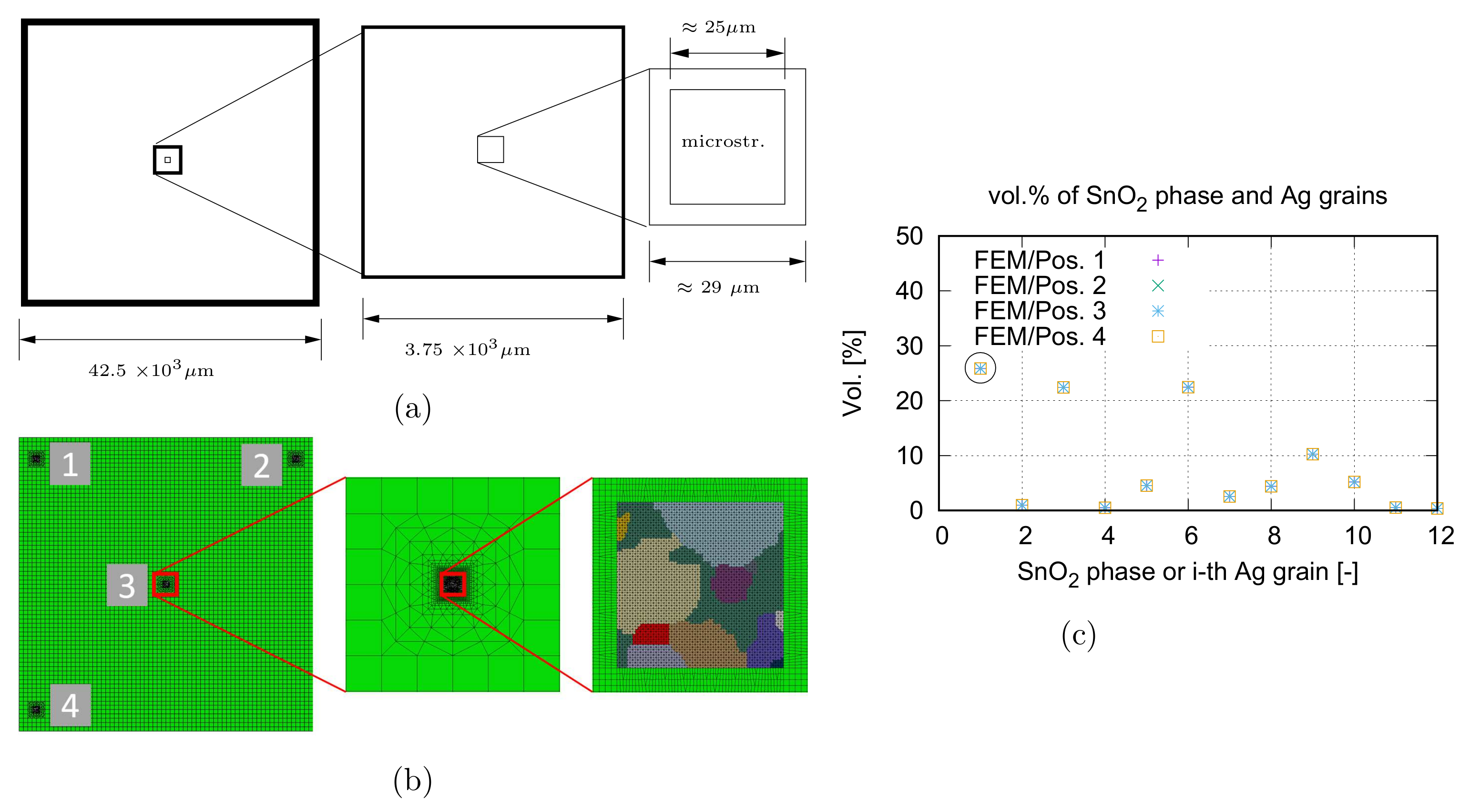
Figure 3a is the aforementioned selected microstructure cut-out for the numerical volume searching process.
Figure 3b schematically presents the macroscopic cross section of a green body sample with a radius of 42.5 mm. In
Figure 3b, “z” and “r” show the axisymmetric and the transverse direction, respectively. The black square presents the whole microstructure, i.e.,
Figure 3a. During the search for a position for the microstructure with 17 vol.% SnO
2, the step length in “r” direction is 0.0741 μm. This step length corresponds to the length presented by one pixel in our original EBSD image (
μmm per pixel).
Figure 3c presents the numerical volume searching result. From
Figure 3c, it is clear that the SnO
2 phase volume fraction is indifferent to the position of the microstructure in the macrostructure. The phase volume fraction converges to its area fraction in the 2D microstructure (25.5 vol.%).
Figure 3d shows an enlarged view of the region marked by a circle in
Figure 3c. This convergence means that it is not possible to find a position for the given microstructure with 17 vol.% SnO
2.
Figure 3c is the result from our numerical searching, it would be more convincing, when phase volumes in FE simulations show the same independence on the microstructure position. Since two-scale prediction is preferred in our work, the aforementioned indifference is also proved by a two-scale FE meshing.
Figure 4a illustrates the dimensions of the figures in
Figure 4b. The same microstructure cut-out (
Figure 3a) is embedded in four different positions inside a macrostructure as shown in
Figure 4b, left. The meshing of the transition zone is shown in
Figure 4b/middle for connecting positions with the macrostructure. For the connecting positions with the microstructure, the meshing of the transition zone is presented in
Figure 4b, right. Each pixel in the microstructure is meshed with 2 triangles (
Figure 4b, right) so that the volume covered by a pixel is identical for the numerical search (
Figure 3) and for the FE simulation (at a specific position of the microstructure on the macro cross section). The resulting volume fractions of the SnO
2 phase and 11 Ag grains are shown in
Figure 4c. For the SnO
2 phase, its volume fraction is marked by a black circle. It is pointed out that the phase volume fraction indifference to the microstructure position is valid for any phase and any microstructure size in an axisymmetric (2.5D) analysis. To prove the universality of this convergence, a mathematic proof is presented in
Appendix A.
2.1.1. Crystal Plasticity Modeling
For a good numerical prediction of the polycrystalline material, like our ODS Ag/SnO
2 MMCs, different micro mechanisms should be taken into consideration, like the anisotropy, the interaction among grains, and the dislocation activation, as well as the heterogeneity. Large plastic deformation on the microlevel requires a material model, which can describe the local distorsion and dilatation well. The elasto-visco-plastic material model from the crystal plasticity is suitable to mechanically simulate the Ag phase deformation behavior on the microscopic level. To realize FE simulations, a user defined sub-routine (UMAT in ABAQUS) was developed at the Institute of Mechanics (IFME Institute) of Otto-von-Guericke-University Magdeburg, Germany [
7,
16,
26,
27]. To be simple, the applied model is briefly described as follows.
Elastic Law
A finite anisotropic linear elastic law is used (Equation (
1)), in which the 2nd Piolar-Kirchhoff stress tensor
is a function of the Green strain tensor
E:
In Equation (
1),
and
I represent the 4th order elasticity tensor and the identity tensor, respectively.
F denotes the deformation gradient tensor, which can be further multiplicatively decomposed into
and
P, where
P indicates the plastic transformation [
28,
29], and
is defined as
. If
is identified, this (
) leads to the same decomposition suggested by Lee (1969) [
30], i.e.,
. This elastic law (Equation (
1)) is not constant in time after yielding. It is convenient to transform it into a time-independent law:
Flow Rule
The flow rule is taken from the finite crystal visco-plasticity theory, in which the time evolution of
P is specified in terms of the shear rate
and the Schmid tensors
with a certain slip system
.
, the Schmid resolved shear stress
and
are given as:
respectively [
31].
and
correspond to the reference shear rate and the critical resolved shear stress. For a given spatial velocity gradient
, the flow rule can be formulated in terms of
,
with the Mandel stress tensor
.
Hardening Rule
The Kocks-Mecking hardening rule [
32,
33] is applied, which is a type of the Voce rule and emphasizes the mechanisms of the dislocation density growth, the accumulation and the density decrement. The ansatz applied here has the form
is the work hardening rate near to the yielding point.
is an input material parameter and can be identified from the experiment [
33].
is a material constant (
). Other values of
are possible, but it should be kept in agreement with the order of magnitude expected from the dislocation theory [
33]. The reference shear rate
is a constant.
Homogenization
RVE is used for the microstructure in the current work in order to achieve the transition from the micro to macro variables. The macroscopic material variables are obtained through the homogenization of the corresponding micro fields. Based on the postulate of the work equivalence on the micro and the macro scale [
34], the global first Piola-Kirchhoff stress (
) is related to the local one (
) by
2.2. A Numerical Method to Match Real Composition for Microstructure Cut-Outs
Concerning the physical background of our method to modify the microstructure, it can be referred to
Appendix B. The precondition for the application of our method is that the representativeness of the microstructure is already fulfilled to a certain extent. Here, the aim is to improve the representativeness and put emphasis on the phase volume ratio matching the reality exactly. To achieve a desired volume fraction for a given phase, the basic idea is the alteration of the boundary pixel color of this phase, i.e., our method BPCA. When the volume fraction of the considered phase is larger than the real composition, the color of its outer boundary pixels will be changed into its neighboring pixels’ colors. This method is also suitable for the-other-way-around case, i.e., when the volume fraction of a considered phase in a cut-out is smaller than the value in the real composition. In this case, colors of some neighboring pixels would be changed to the pixel color of this considered phase. The ASCII format is preferred for this color changing process. A code was developed to execute this modification process.
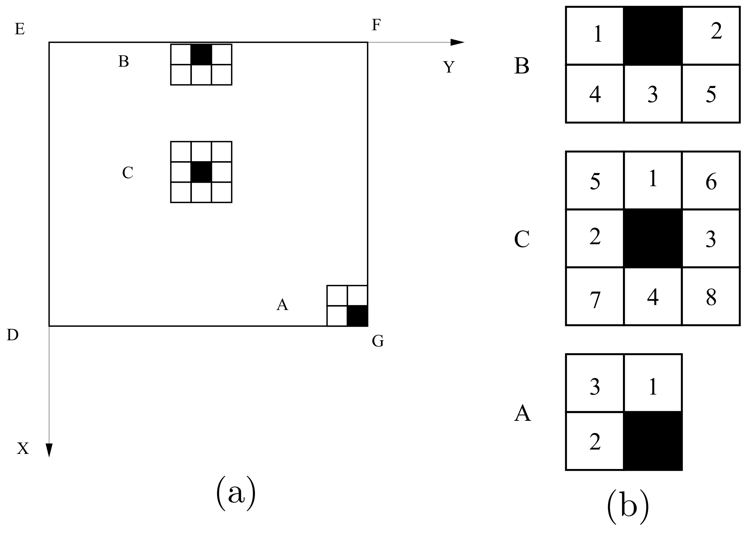
In the current work, each pixel is square shaped, i.e., a pixel presents the same absolute dimension in both horizontal and vertical directions.
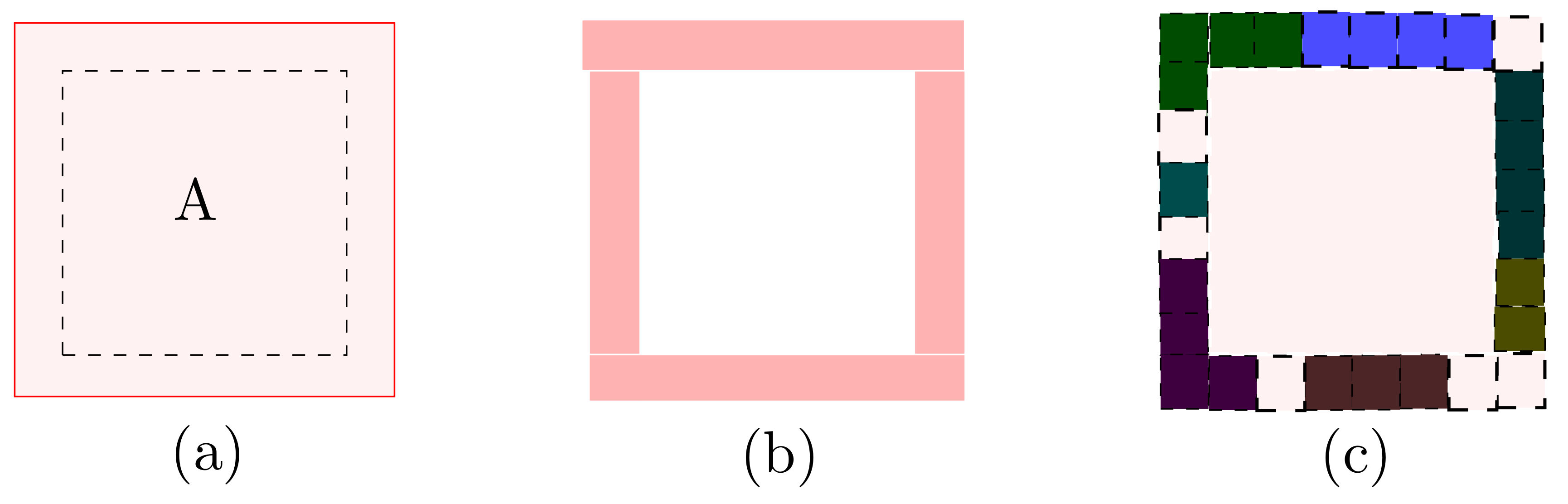
Figure 5a schematically shows a considered pixel (in black square) with its neighbors in an image in the ASCII format. The region DEFG in
Figure 5a presents a microstructure. The point E coincides with the coordinate origin. In
Figure 5a, the pixel shown in a black square is the current considered pixel. For pixel types A, B, and C in
Figure 5a, the number of total neighboring pixels is used as the categorizing condition. In our example, the SnO
2 particle phase has a higher volume fraction than the real one. The color alteration will happen only to the outer boundary pixels of the SnO
2-phase. Such pixels have neighbors which present Ag grains. If neighboring pixels have more than one different colors, a priority criterion should be given to determine the new color for the considered pixel.
Figure 5b demonstrates one of the possibilities. In
Figure 5b, the smaller numbers have priority compared to larger numbers. Supposing that the particle phase has a smaller volume fraction than the real one, the pixel color assignment would be easier than in the aforementioned case. The neighboring pixels (Ag grain pixels) would just change into the color black. No priority for the color assignment is required.
It is supposed that a 2D image has
and
pixels in the X and Y direction, respectively (for directions, see
Figure 5a).
and
present integers. The number of total pixels will be
. The pixel position can be identified as
with
,
and
. Each pixel with a square shape has four peak points. They can be presented as four nodes with possible coordinates of
to
. The
x and
y values in
to
have ranges
and
in the X and Y direction, respectively. To reach the real material composition,
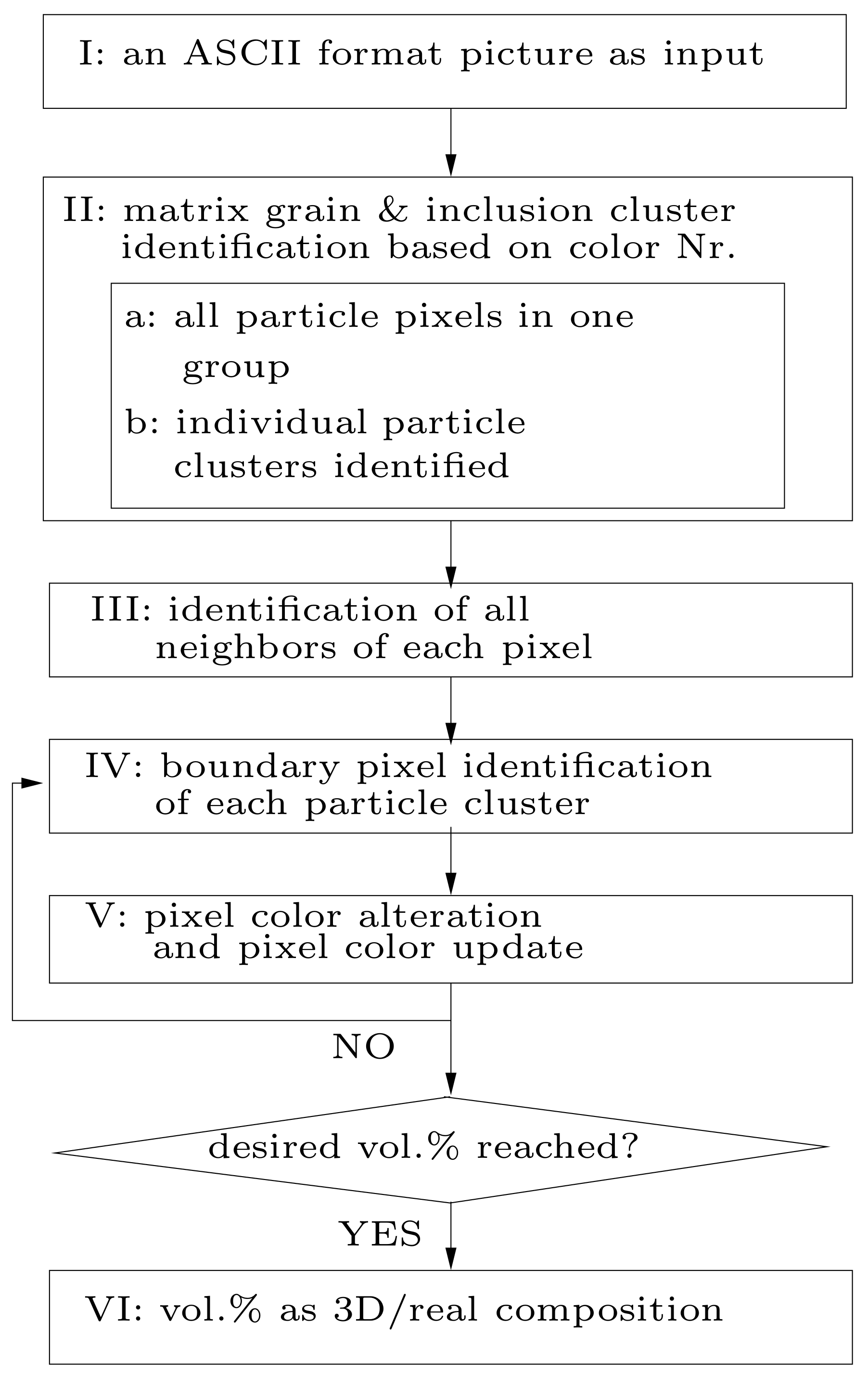
Figure 6 describes this modification process in 5 steps (I–V):
For step-I, the free software GIMP with an open access is used. The given example (
Figure 2c) possesses 171 Ag grains. It means that 172 color numbers (172 pixel groups) are enough to identify every Ag grain and the SnO
2 phase for step-I. For a more complex structure with more than 256 grains/clusters, our method is still applicable. The method described in step-II-b can be used to separate grains/clusters with the same pixel color number.
In step-II, all the information concerning a pixel should be coupled (linked with each other). It includes the pixel position (), the pixel group number, four node coordinates ( to ) and the color number. The number of total pixel groups is identical to the number of total pixel colors at this stage. It means that pixels with the same color are in the same group, even though they may belong to different pixel groups later on. Step-II-a is automatically done by reading the input data, since all the particles have the same color. Step-II-b is a key point for the pixel color alteration. A “glue” process is iteratively applied here. As the starting point, the code takes an arbitrary pixel (pixel-a) in the considered range. This range means a considered phase or grain. The aforementioned starting pixel belongs to a certain cluster A. It means that different clusters will be identified from the particle phase. Each cluster starts with a pixel. The cluster A is also the pixel group A. If another pixel fulfills two conditions: (i) being inside the considered range (black color in the example); (ii) having at least one shared node ( to ) with the pixels inside the pixel group-A (already identified), this pixel will be included to the pixel group A. Thus, the number of total pixels in group A increases. Then, the code will search for the next possible pixel. During the search, there are parallel sub-groups for a pixel group, since the iterative loop is done for pixels one after another. It begins with and , and goes to and . After the pixel , will be the next pixel to be considered. It implies that this “glue” process includes: (a) sticking pixels to pixels; (b) sticking sub-groups to sub-groups; (c) sticking pixels and sub-groups. As a final result of step-II-b, individual particle clusters are identified.
Step-III links together the information attached to a pixel. It can be relatively easily done compared to the step-II. For each identified particle cluster, a new pixel color is required to distinguish it from other clusters and Ag grains. When it requires more than 256 grains/clusters in a microstructure, some grains/clusters will have the identical pixel color number. In this case, in order to track each grain/cluster, one can resort to the integer assigned by the code (mentioned in Step-I). No neighboring grains/clusters share the same pixel color number. The considered field is the microstructural features of alloys. The possibility should be nearly zero for one grain/cluster with more than 255 neighbors. Another way would be to use the colored pixels. For such pixels, 3 numbers (red-green-blue RGB color) describe one pixel color. But the work of the pixel color comparison for the code will be much higher than the comparison work used by the greyscale color.
Step-IV identifies the outer boundary pixels of an individual pixel group inside the considered range. In our case, this range refers to SnO
2 clusters. This step is another key point of the algorithm. The criterion is that a SnO
2 pixel has at least one neighbor with a pixel color number of Ag grains. As a verification, all the pixels on the outer boundary must have at least one shared node with one of the other pixels in the same pixel group (the boundary pixel group, not the cluster pixel group). Each boundary pixel group composes a closed loop which encloses the given grain/cluster. Such closed loops can be referred to, e.g., the particle surrounded by a green oval line in
Figure 7b,e (for particles inside the cut-out, not the ones cut by the microstructure edges). It is pointed out that some SnO
2 boundary pixels are not shown in
Figure 7b,c,e. Such pixels locate on the edge of the microstructure cut-out. By adding such pixels in
Figure 7b,c,e, closed loops will also be shown for particles cut by the microstructure edges. Such images with closed loops for all the particles would not be presented in the current work, since it is just a matter of choosing the image illustration and has no influence on our method. SnO
2 boundary pixels located on microstructure edges do not have Ag neighbors, so they are excluded of the pixel color alteration process. It also means that their color is maintained during the pixel color modification process.
Step-V alters and updates the pixel colors. If the desired volume fraction is not yet reached, the update of the neighborhood information will also be done so that it is ready for the next layer of the BPCA process. As a final result, the real composition is achieved, and the pattern of the original microstructure is maintained, as well.
In our early work [
35], where no method description is available due to predefined page limit, a small cut-out with only 11 Ag grains and 3 SnO
2 clusters (upper left corner in
Figure 2b) was used to test the aforementioned BPCA process. By taking
Figure 2c (80
2 μm
2) as the starting microstructure,
Figure 7a–f show the intermediate and the final results of this modification process. Based on our experience, the grain and particle boundaries are already well recognizable in an image with 200
2–300
2 pixels for the aforementioned size (80
2 μm
2). The particle phase amounts to 23.96 vol.% in
Figure 2b,c.
Figure 7a shows the identified particle phase as a whole. It means that all the particle pixels are in the same pixel group at this stage and have the same color black.
Figure 7b presents the boundaries of 25 identified particles, where each individual one has its own color. Here, only the pixels of the particle phase (on particle boundaries) are shown, which have neighboring pixels belonging to Ag grains. It is pointed out that some particles may not be well identified by naked eyes in
Figure 7b.
For a given microstructure, the number of total pixels
is fixed.
i refers to the number of an individual particle/cluster in a given microstructure. In our case,
(
Figure 7b,c,e).
denotes the
cluster volume/area fraction.
presents the SnO
2 phase volume/area fraction, i.e.,
. For the given example (
Figure 7),
= 23.96% before the modification (
Figure 7a) and
= 17% after the modification (
Figure 7f).
is the difference of the particle phase volume fraction between the original 2D microstructure cut-out and the 3D/real one, i.e.,
.
presents the total pixel number of the ith particle cluster at the beginning of this modification process, and
. If
indicates the number of total modified pixels on the boundary of the cluster
i, then (
):
In our example (
Figure 2c),
,
and
. The largest particle cluster has 2882 pixels (
). For this particle, it holds
and
The number of total SnO
2 pixels with a color alteration will be
for the particle phase in our example. It also means that a particle with a smaller volume would have fewer pixels changed into Ag colors. As a result, all particles in the original microstructure are involved in the BPCA process, as well as maintained in the final microstructure (after the pixel color modification). From
Figure 7b,c, some pixel colors of the SnO
2 phase are changed into the color of polycrystalline Ag grains. These Ag grains must include pixels which are neighbors of particle pixels in
Figure 7b. The involved pixels in
Figure 7b,c are at the same positions. But each grey colored pixel in
Figure 7c has the property of a Ag grain, not the property of SnO
2 anymore. It is worthy to mention that some pixels in
Figure 7c might not be identified by the naked eyes, since the color contrast to the white background is too weak. After the pixel color change for the first layer (outer boundaries of particle clusters), the resulted microstructure, not shown here, is similar to
Figure 2f, which is an intermediate result, since the SnO
2 phase has not yet reached its real volume fraction. The pixel color modification should go further, i.e., to the 2nd layer or (N + 1)th layer in order to reach the desired phase volume fraction. Before going to the next layer, the neighborhood update in the code is necessary for pixels located on particle boundaries, since the boundary pixels of the SnO
2 phase are not identical to the ones before the color change. All the neighbors of a pixel on boundaries of clusters need to be identified.
Some clusters of the SnO
2 phase might be sub-divided into sub-clusters due to the pixel color changing. If so, the presented code can still identify all the outer boundaries for the whole SnO
2 phase, since the iterative process in the code goes through all the pixels in the considered range, i.e., all pixels in color black. The particle marked with a red dashed oval line in
Figure 7b is separated into two particles (particles marked with a red oval line in
Figure 7e) after the pixel color alteration. Analogous to
Figure 7a,b,
Figure 7d,e illustrate the modification process for the 2nd layer, the starting state of which is
Figure 7d for the boundary pixels of the particle phase. The 2nd round of searching boundary pixels includes only the particles, the
of which in Equation (
7) is not yet reached. The final result is presented in
Figure 7f, which is completely ready for meshing. Based on our experience, the particle volume fraction after meshing, i.e., calculated from elements, has a deviation to the value calculated from pixels less than 1%, which is inside an acceptable tolerance. In our case, the former is slightly lower than the later. In such a case, one tip would be to modify the given cut-out to a particle fraction 0.5% higher than the real one.
The next work is to apply the resulted image in an axisymmetric (2.5D) two-scale FE model to simulate the extrusion process. Such FE calculations (phase field method [
36]) should predict the recrystallization mechanisms of Ag grains. Special attention will be paid to the formation of
-twins in Ag phase. After twice extruded, the resulting microstructure will be loaded under tension to investigate the
-twins influence on the texture evolution. FE results will be given in further reports.
Our BPCA method is also applicable to modify N (N > 1) phases in a microstructure. Each phase can be polycrystalline. In such a case, one way would be to perform BPCA for phases one after another. During the modification of the
phase (1 < m ≤ N), the pixels, which belong to the already modified pixels of phase k (1 ≤ k < m), should be preserved, i.e., not taking part in the BPCA procedure. This is to guarantee the correct volume/area fraction for the previously modified phases. Our code does not include this function to preserve pixels, since no such necessity, i.e., no modification of N phases, appears in our works until now. As mentioned in
Section 1, our method is also applicable to modify the size or size distribution of a phase or several phases, since it goes through every pixel and the pixel color alteration changes the size of the phase/grain. If a grain/cluster has necking regions (narrow regions between two or more broad regions), the BPCA process can separate it into two or more grains/clusters (e.g., the particle surrounded by a dashed red oval line in
Figure 7b,e). It indicates that the distribution of grains/clusters is modified. It is pointed out that the modification of the phase distribution is not the aim of the current work. Simply, a particle with a necking region is separated by the BPCA process (
Figure 7b,e). The original particle distribution pattern is mostly maintained in our example. As mathematically shown in
Appendix A, the phase volume fraction in a microstructure can be indifference to the microstructure’s position in an axisymmetric (2.5D) analysis (
Figure A1 in
Appendix A). Our microstructure modification method is even more meaningful, since the resulting microstructures can be applied in 2D, as well as in axisymmetric (2.5D) FE simulations.
2.3. Further Applications
To show the universality of the numerical finding, i.e., the phase volume fraction convergence in an axisymmetric simulation to its 2D area fraction, and to train our code, the same progress as given in
Figure 7 is applied for another three material microstructures.
As a kind of tool materials, tungsten carbide/cobalt (WC-Co) exhibits properties with exceptional combinations of hardness, toughness, strength and wear resistance. They are important for industrial manufacturing and daily life. Hard metal inserts share half of the market for cutting tools [
37]. For applications of hard metal components, such as cutting tools and drawing dies, the cemented WC-Co share about 98% of the market today [
38]. Concerning these WC-Co tool materials, most published results are for the ones with tungsten carbide phase as the major phase (matrix). Some of our studies concentrate on the deformation and the damage evolution in Co/WC/diamond MMCs with Co as the matrix. Our sample material, much less studied as compared to those with WC as the matrix, is also a kind of tool materials, e.g., for cutting and grinding. Such materials can show both ductile and quasi-brittle behaviors [
39,
40].
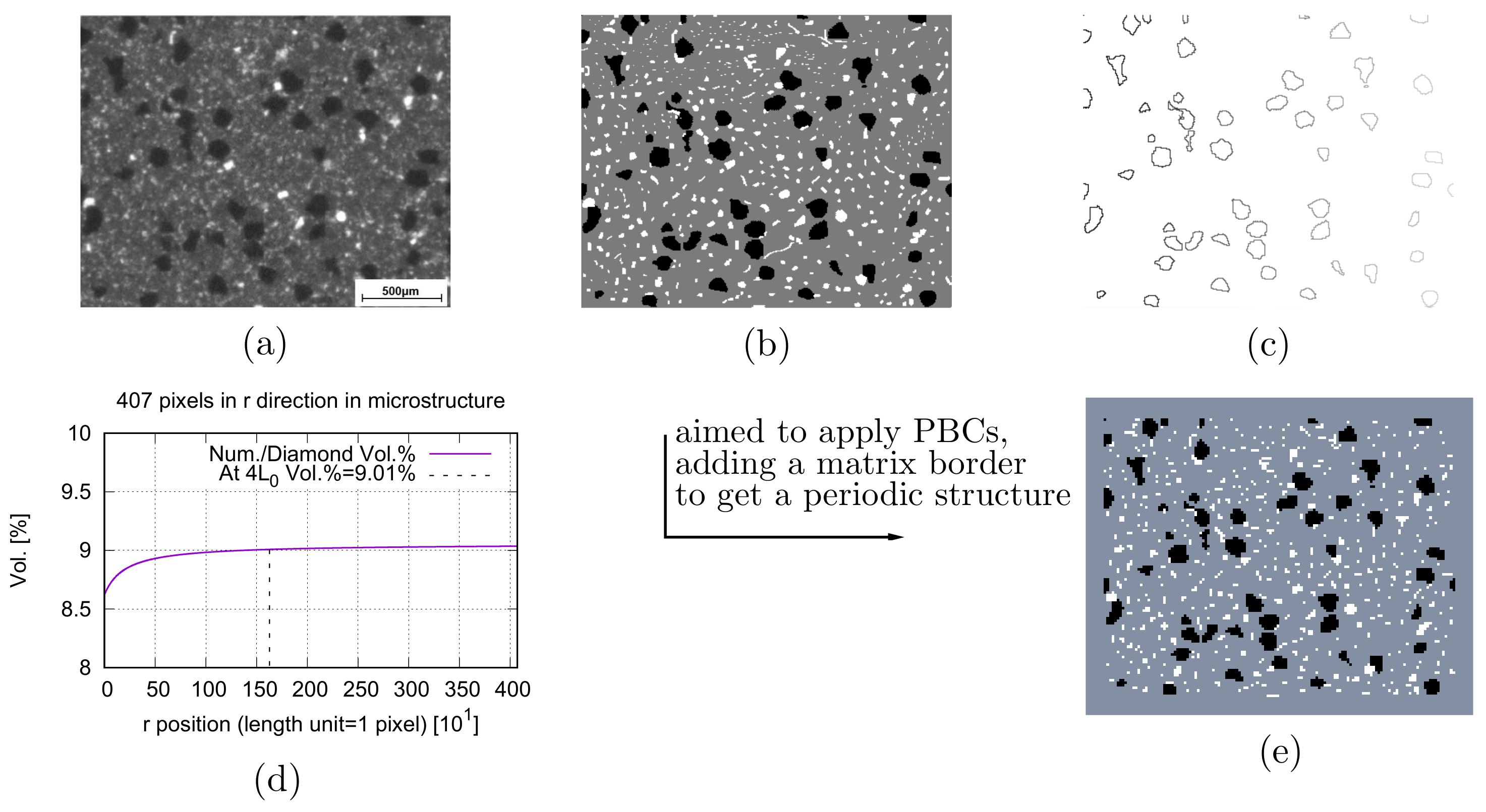
Figure 8a presents a real 2D microstructure cut-out of a Co/WC/diamond composite with 9.06 vol.% diamond, where the volume ratio of Co:WC:diamond is 90:5:5 for the commercial sample. After the pixel handling,
Figure 8b with a pixel resolution of 407 × 322 illustrates the same microstructure as given in
Figure 8a.
Figure 8c shows the identified boundary pixels of the 54 diamond particles, where each individual piece is assigned with a non-equal pixel color number. The diamond phase volume fraction in an axisymmetric analysis is presented according to the microstructure position in the macrostructure, where the length of one pixel is used as a unit length. The vol.% of the diamond phase with a value of 8.62 vol.% at the beginning of the calculation and 9.05 vol.% at the end (
Figure 8d) converges to its 2D area fraction of 9.06% in the microstructure. At the position with r = 4
, i.e., r =
unit lengths, the diamond volume fraction is 9.01 vol.%. There exist WC particles with a non-negligible volume fraction with a sub-micro-size, which cannot be captured by a microstructure. In this case, the size and strengthening effect of sub-micron sized WC particles are taken into consideration by using the homogenized matrix (Co + sub-micron-sized-WC) in the FE simulation, where the mechanism-based strain gradient theory [
41,
42] is applied in an axisymmetric simulation. The resulted homogenized matrix is further used in 2D FE simulations for the local damage evolution, since only a measured 2D local strain map is available due to limited experimental data. As mentioned in
Section 1, the analysis types, i.e., 2D, axisymmetry and 3D, have coexisted and will further coexist. For one-scale micromechanical FE simulations, periodic boundary conditions (PBCs) should lead to better predictions than homogeneous ones, since the latter set too strong constraints for degrees of freedom on boundary nodes. To apply PBCs, it requires periodic structures. Usually, real microstructures possess randomness, i.e., no periodicity of the structure. In simple cases, as
Figure 8a, artificial modification might be used to obtain the periodicity.
Figure 8e is a special periodic structure obtained by adding a border of
Figure 8b. For
Figure 8e, the PBCs can be used, but not for
Figure 8b. In order to find out a better way of FE prediction, it would be beneficial to compare the inaccuracy introduced by this artificial modification of the real microstructure and by the strong constraints of homogeneous BCs.
It is of technological and research interest to study metal alloys with microstructures consisting of two ductile phases, e.g.,
/
-titanium alloys, duplex steels, Cu–Nb, Ag–Ni, etc. [
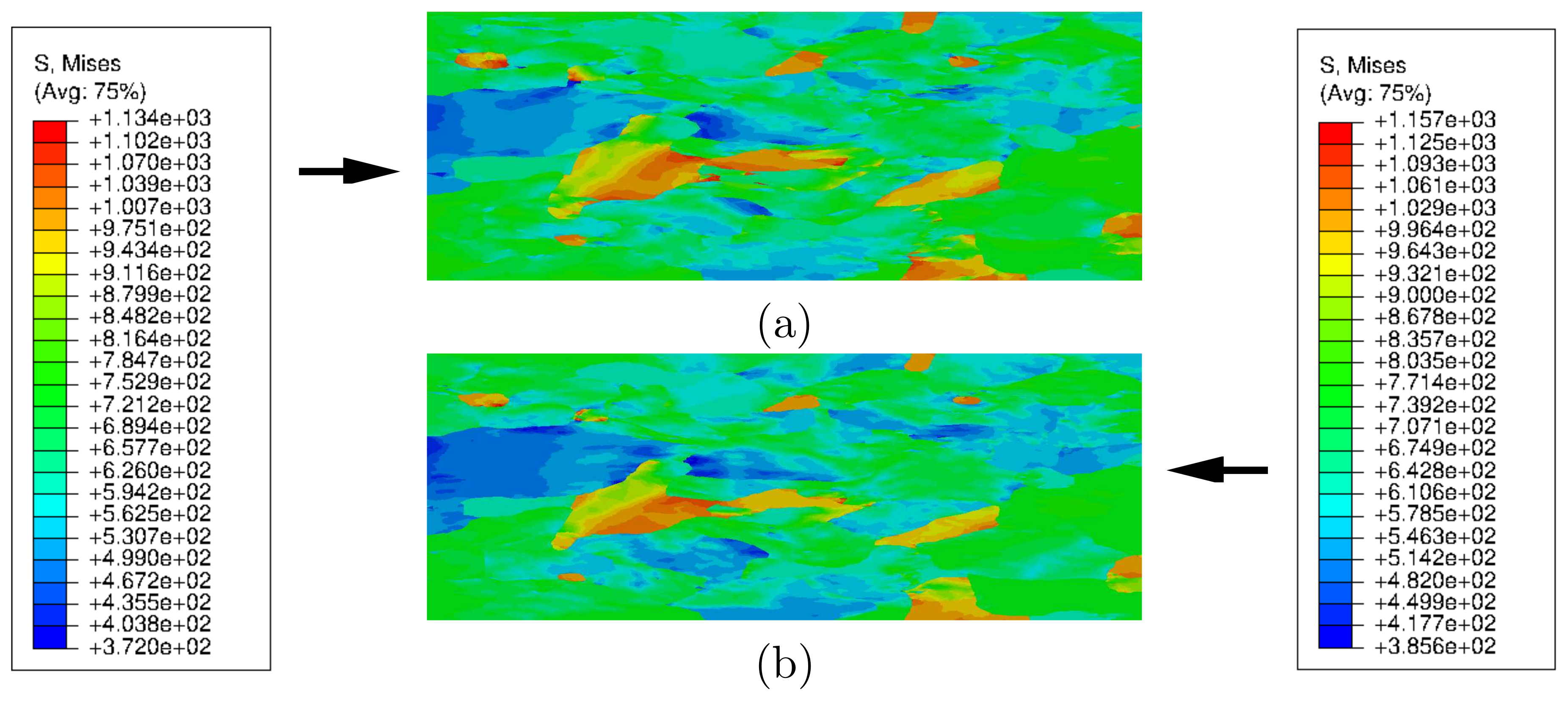
43]. Thereby, properties of crystallites in both phases will be “combined together” to determine the macroscopic properties of the mixture. The individual properties of each phase will be changed due to the presence of the other phase. The physical and mechanical mechanisms for the aforementioned two cases are of interest for the processing of materials and for the prediction of the deformation behavior. Commentz et al. [
43] experimentally and numerically studied the micro texture evolution and global stress-strain behavior of
-Fe/Cu MMCs according to
-Fe:Cu volume fractions, where both phases are polycrystalline. Their numerical study is based on a viscoplastic self-consistent (VPSC) model, which can be categorized into a physical approach. Schneider et al. [
7,
16] numerically studied the texture evolution by using FE simulations with an elasto-visco-plastic material model in a crystal plasticity approach, i.e., an approach by using theories of continuum mechanics. After meshing, the applied real microstructure has about 23 vol.%
-Fe grains (element volume) for an Fe17-Cu83 (Fe17 vol.%–Cu83 vol.%) MMC [
7].
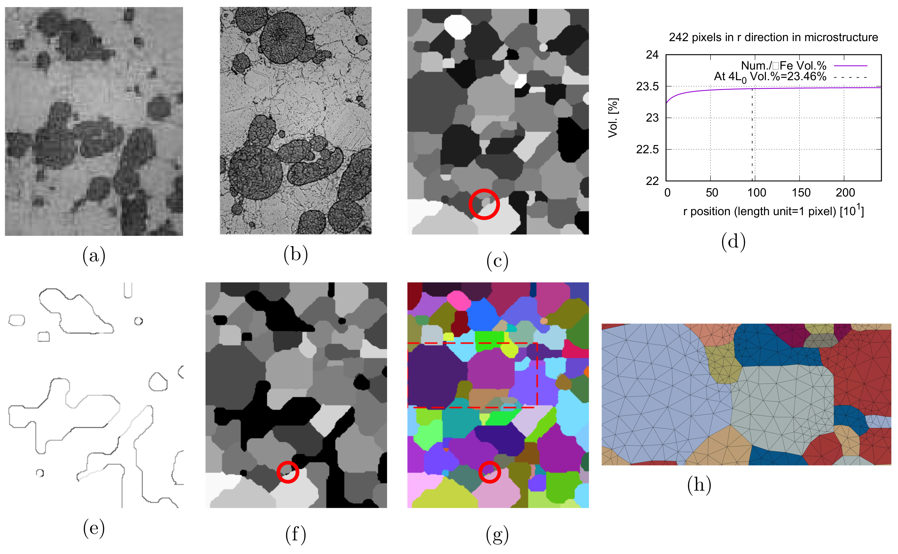
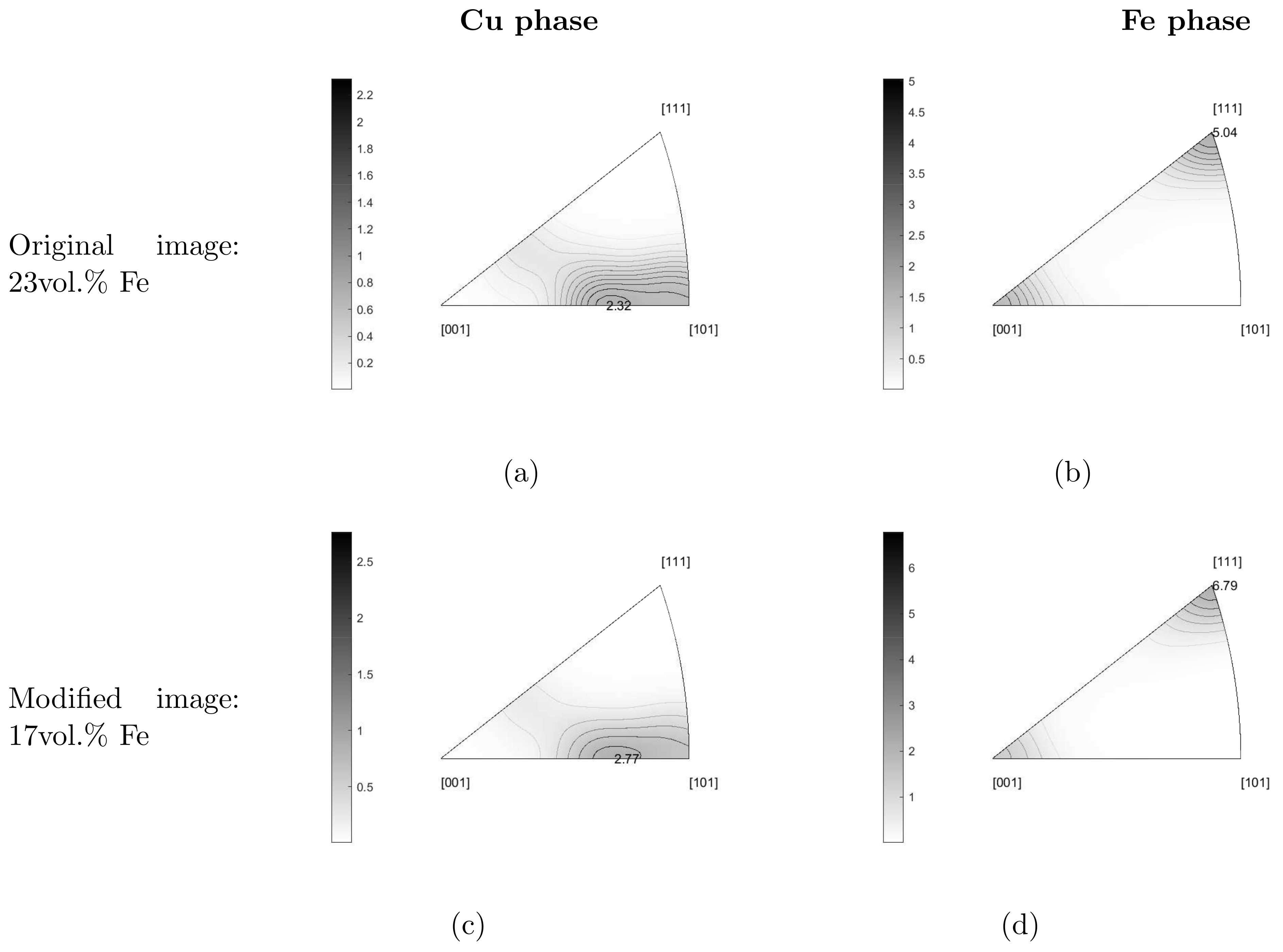
Figure 9a presents a microstructure cut-out of Fe17-Cu83 MMC [
43] and
Figure 9b is the same one with a better pixel resolution but a slightly smaller size [
7,
44]. Based on the morphologies given in
Figure 9a,b,
Figure 9c with the pixel resolution of 242 × 301 is obtained after the pixel handling [
7], where
-Fe has an area fraction of 23.49%. By an artificial and manual alteration of polycrystalline
-Fe into clusters with the same pixel color number, i.e., not polycrystalline
-Fe anymore (resulted image resembles
Figure 9f and will not be shown here). According to the structure position in the r direction in
Figure 3 for an axisymmetric analysis,
Figure 9d illustrates the volume fraction convergence of the
-Fe phase to its 2D area fraction. In
Figure 9d, the length of one pixel is used as a unit length. At the position with r = 4
=
unit lengths, the
-Fe volume fraction is 23.46%.
Figure 9e,f illustrate the identified boundary pixels of individual
-Fe clusters assigned with different pixel color numbers and the microstructure with 17 vol.%
-Fe, i.e., real one, after the BPCA process. For meshing, the originally polycrystalline
-Fe phase is needed, which is given through overlapping
Figure 9f by
Figure 9c for the
-Fe phase. The resulted microstructure with polycrystalline grains for both phases is demonstrated in
Figure 9g, where the colored pixels can be easily assigned during the overlapping by the code. The small
-Fe grain enclosed by a red circle in
Figure 9c becomes tiny after the application of the BPCA procedure (
Figure 9f,g). It is user dependent, whether such a tiny grain should be meshed, since for both cases the whole calculation amount will be acceptable in a 2D or axisymmetric simulation. By using
Figure 9c,g, FE predictions are compared for the homogenized stress-strain curve, the texture and local strain distribution. After meshing, the volume fraction of the
-Fe phase is 17.31 vol.%. It means that the volume fraction difference is 0.3 vol.% before (pixel) and after meshing (elements). The geometrical adaptive meshing for the region marked by a red rectangle with dashed lines in
Figure 9g is presented in
Figure 9h (meshing software [
45]). It is worth mentioning that from
Figure 9c to the geometrical adaptive meshing for the whole structure took only a few hours. The
-Fe vol.% (element volume) has a deviation less than 0.5%, compared to the real one (pixel volume). By finely meshed structures, this value can be closer to the real one and the FE simulation can still properly run, since the total number of elements in an axisymmetric or 2D meshing is still within the calculation capacity, while it often exceeds the calculation capacity for 3D cases.
Austenitic-ferritic steel is often used in high temperature environments. For such materials, chromium oxide scale is widely used as a protection film to resist high-temperature oxidation [
46], where “scale” means an oxidized film. Aluminum oxide scale exhibits substantially greater thermodynamic stability than chromium oxide scale in many aggressive environments. For the Al alloyed austenitic steels, the volume fraction of the austenitic phase and of the ferritic phase is significantly influenced by the amount of alloyed Al elements, which is a kind of typical ferritic forming (chemical) elements. Unlike MMCs, e.g., Ag/17 vol.%SnO
2 and
-Fe17-Cu83 mentioned above, the exact austenitic-ferritic volume ratio on the microscale cannot be accurately determined by the weight or volume ratios of alloyed chemical elements.
Figure 10a presents a microstructure cut-out of an austenitic-ferritic steel with the austenitic phase shown in lighter color. After the pixel handling (
Figure 10b with a pixel resolution of 320 × 240), the ferritic phase has an area fraction of 21.70%. In
Figure 10c, the ferritic phase volume fraction, which starts with the value of 23.43% and ends at 21.80%, converges to its 2D area fraction of 21.70% in an axisymmetric analysis. At r = 4
= 960 μm, the austenitic phase area fraction is 21.80%.
Figure 10d presents the identified boundary pixels of the austenitic phase in
Figure 10b. To show the phase volume convergence in an axisymmetric analysis, all the above three numerical calculations,
Figure 3c,
Figure 8d, and
Figure 9d, present the case that the original phase volume fraction is higher than the real one. For
Figure 10b, it is assumed that the desired volume fraction of the austenitic phase is higher than the one in the original microstructure. In
Figure 10e, the austenitic phase amounts to 30.10%, i.e., a dual-phase steel (austenitic vol.% no less than 30%). To illustrate that the original morphologies are maintained,
Figure 10f shows the overlapping result of
Figure 10d (in red) and
Figure 10e (in blue). It means that our BPCA method can improve the real microstructure representativeness, as well as can maintain the main characteristics of the original morphology.


 ,
, 