Article

Interplay of Active Stress and Driven Flow in Self-Assembled, Tumbling Active Nematics

Department of Physics, Hong Kong University of Science and Technology, Clear Water Bay, Kowloon, Hong Kong, China
*
Author to whom correspondence should be addressed.
Crystals 2021, 11(9), 1071; https://doi.org/10.3390/cryst11091071
Submission received: 31 July 2021 / Revised: 30 August 2021 / Accepted: 31 August 2021 / Published: 4 September 2021
(This article belongs to the Special Issue Self-Assembly in Liquid Crystalline Materials)

Abstract

:
Lyotropic chromonic liquid crystals (LCLCs) are a special type of hierarchical material in which self-assembled molecular aggregates are responsible for the formation of liquid crystal phases. Thanks to its unusual material properties and bio compatibility, it has found wide applications including the formation of active nematic liquid crystals. Recent experiments have uncovered tumbling character of certain LCLCs. However, how tumbling behavior modifies structure and flow in driven and active nematics is poorly understood. Here, we rely on continuum simulation to study the interplay of extensile active stress and externally driven flow in a flow-tumbling nematic with a low twist modulus to mimic nematic LCLCs. We find that a spontaneous transverse flow can be developed in a flow-tumbling active nematic confined to a hybrid alignment cell when it is in log-rolling mode at sufficiently high activities. The orientation of the total spontaneous flow is tunable by tuning the active stress. We further show that activity can suppress pressure-driven flow of a flow-tumbling nematic in a planar-anchoring cell but can also promote a transition of the director field under a pressure gradient in a homeotropic-anchoring cell. Remarkably, we demonstrate that the frequency of unsteady director dynamics in a tumbling nematic under Couette flow is invariant against active stress when below a threshold activity but exhibits a discontinuous increase when above the threshold at which a complex, periodic spatiotemporal director pattern emerges. Taken together, our simulations reveal qualitative differences between flow-tumbling and flow-aligning active nematics and suggest potential applications of tumbling nematics in microfluidics.

Graphical Abstract

1. Introduction

Liquid crystal (LC) is a state of condensed matter intermediate between disordered liquid phase and highly ordered crystalline phase [1]. A commonly studied LC phase is called the nematic phase in which anisotropic units, namely mesogens, of the LC develop long-range orientational ordering but remain spatially disordered [2]. Owing to the sensitivity of its orientational ordering relative to external stimuli and internal physicochemical events, nematic LCs have found wide applications in display, photonic devices and biosensing [3,4]. More recent applications of nematic LCs include directed self-assembly of colloids [5,6,7] and amphiphilic molecules [8,9]. In these applications, equilibrium structures and their thermodynamic stability at different conditions are concerned. In the recent decade, there is a trend to understand and control transport and dynamics of nematic LCs [10,11,12]. On the one hand, applications of nematic LCs in microfluidics, which require a deep understanding of nematic flows, are in its early stage [13,14,15,16,17,18]. On the other hand, recent discoveries of LC phases in in vivo and in vitro biological systems have rejuvenated the research of LC flows [19,20,21]. Due to the nonequilibrium nature of these biological systems, they are termed “active liquid crystals”, which has seen a surge of interests in recent literature [22,23,24,25]. In some types of active nematic LCs, their constituents can self-propel, as is the case for two-dimensional sheets of microtubule and kinesin [26], or actin and myosin [27] and dense bacteria suspensions [28]. Another class of active nematics is often called “living nematic” in which bacteria are swimming in a nontoxic, lyotropic chromonic LC [29,30,31,32]. An analogous system consists of active biopolymers suspended in a passive colloidal nematic LC [33]. Despite the fact that a rich body of literature is devoted to understanding the intriguing phenomena of active LCs, its rheology remains much less studied [34,35].
Lyotropic Chromonic LCs (LCLCs) are comprised of disk-like molecules in a solution, stacking into self-assembled cylinders, which serve to form different LC phases including nematic and columnar phases [36]. Examples of LCLCs are disodium cromoglycate (DSCG) solutions [37] and Sunset Yellow solutions [38]. These types of nematic materials exhibit disparate elastic constants. In particular, experiments have shown that, in the nematic phase, LCLC’s twist modulus K 2 is one order of magnitude smaller than splay and bend moduli [39]. This feature has resulted in the spontaneous formation of symmetry-broken chiral structures in this achiral system [40,41,42,43]. The unusual material properties and biocompatibility of certain LCLCs have shown its promise in applications in, for example, optics [44], sensing [45], microfluidics [46] and active matter [47]. However, our knowledge of its rheology is limited. The response of a nematic liquid to a simple shear flow can be categorized into two types. For a flow-aligning nematic with Leslie viscosity coefficient α 3 < 0 and α 2 < 0 , directors can find a stationary within the shear plane orientation under a high shear rate, making a so-called “Leslie angle” with respect to the flow direction. For a flow-tumbling nematic with α 3 > 0 and α 2 < 0 , however, directors cannot settle into a stationary orientation and thereby tumble persistently. Recent experiments of nematic DSCG solutions have uncovered its tumbling character, manifested by the emergence of a log-rolling state at intermediate shear rates [48,49]. In this state, directors tend to rotate out of the shear plane and roll with respect to the vorticity direction, reminiscent of logs rolling on the ground [48].
Several active LCs, for instance living nematic, are flow-tumbling. However, how tumbling character, including log-rolling behavior, influences the dynamics of active nematics is overlooked in literature. Recent continuum simulation works have found that flow-tumbling character can suppress activity-driven hydrodynamic instability [50] and can promote more topological defects in two-dimensional active nematics [51]. Another study predicts that the tumbling character can even induce a coherent and spontaneous flow in an LC above the nematic-isotropic transition point [52]. These existing simulation studies of tumbling active nematics, however, use one-elastic-constant approximation. The log-rolling mode is intrinsically a three-dimensional (3D) phenomenon and requires low twist constant [48,53]. To the best of our knowledge, 3D tumbling dynamics in active nematics have not been discussed.
Here, we study spontaneous and driven flows in tumbling active nematics confined to a cell with different anchoring conditions and contrast their behavior to that of flow-aligning nematics. We perform hybrid lattice Boltzmann simulation in order to simultaneously solve Beris–Edwards equation and Navier–Stokes equation. We first validate our method by simulating Couette flow for flow-aligning passive and active nematic within a planar-anchoring cell and by comparing numerical solutions of the Leslie–Ericksen theory. We next study activity-induced spontaneous flows. Our calculations show that for flow-aligning nematics, extensile active stress can drive a net flow in a hybrid alignment cell (planar and homeotropic anchoring condition for each wall) thanks to its viscosity anisotropy. For a flow-tumbling nematic in the same hybrid cell, however, we find that a net flow along transverse direction can be developed in splay-bend tumbling nematic when the log-rolling mode appears at sufficiently high activity level. The ratio between the transverse flow rate and the easy-axis flow rate or the direction of the total flow can be varied by varying activity level. Note that in flow-aligning active nematics, activity and twist do not explicitly interplay because activity promotes solely bend and splay distortions, and these distortions solely give rise to active flows. Our prediction of a spontaneous transverse flow in log-rolling nematics provides a possible mechanism to couple active stress and twist deformation in active nematics.
We further study how activity modifies driven, steady flows and focus on uniform anchoring condition. For a planar-anchoring cell, we find that pressure-driven flow can be enhanced and suppressed in flow-aligning and flow-tumbling nematic, respectively, due to the fact that the directors rotate in opposite handed directions for these two types of nematics. For a homeotropic-anchoring cell, we show that activity can lower the critical pressure gradient at which a “bowser” state can transition into a “dowser” state. By making the nematic tumble more by tuning down the flow aligning parameter, one can also lower the critical pressure gradient.
Lastly, we examine the effect of activity on driven, unsteady flows. Specifically, we consider the unsteady dynamics of a tumbling nematic under a Couette flow. We observe a shear-rate-dependent critical activity, below which the frequency of log-rolling dynamics is independent of activity and above which there is a discontinuous increase in frequency. Such jumps in frequency are attributed to the emergence of a complex, spatiotemporal pattern of the nematic field above the critical activity. Furthermore, we discover a new dimensionless number where different shear-rate systems transition into complex patterns at the same threshold.
In summary, our results highlight several qualitative differences between flow-aligning and flow-tumbling active nematics in terms of spontaneous flows and steady and unsteady driven flows. Our predications of tunable 3D spontaneous flows and digital response of tumbling frequency relative to activity suggest potential applications of tumbling nematics in microfluidics.

2. Methods

2.1. Hybrid Lattice Boltzmann Method

Here, we describe our hybrid lattice Boltzmann method (LBM). The microstructure and hydrodynamic flow of a nematic LC are described by a tensorial order parameter Q and a vector u , respectively. For a uniaxial nematic, it can be written as Q = S ( nn I / 3 ) in which the unit vector n represents the nematic director field, S is the scalar order parameter of the nematic and I is the identity tensor. By defining strain rate D = ( u + ( u ) T ) / 2 and vorticity Ω = ( u ( u ) T ) / 2 , one can introduce an advection term S = ( ξ D + Ω ) · ( Q + I 3 ) + ( Q + I 3 ) · ( ξ D Ω ) 2 ξ ( Q + I 3 ) ( Q : u ) , where ξ is the flow aligning parameter that determines the Leslie angle θ 0 via ξ cos ( 2 θ 0 ) = 3 S 0 / ( 2 + S 0 ) with S 0 being the equilibrium scalar order parameter [50,54]. Therefore, there exists a critical parameter ξ c = 3 S 0 / ( 2 + S 0 ) such that the nematic is flow-aligning when ξ > ξ c , and it is flow-tumbling when ξ < ξ c . This critical flow aligning parameter can also be derived by solving for α 3 = 0 in Equation (A1) in Appendix A.1.
The governing equation of the Q-tensor, namely the Beris–Edwards equation, is written as follows [55]:
Q t + u · Q S = Γ H ,
where Γ is related to the rotational viscosity of the underlying nematic via γ 1 = 2 S 0 2 / Γ [54] and H is molecular field defined as H = ( δ F δ Q I 3 Tr ( δ F δ Q ) ) , which drives the system towards thermodynamic equilibrium with a free energy functional F = V f LdG d V + V f elastic d V + V f surf d S . The first term is the short-range Landau–de Gennes free energy density, which reads f LdG = A 0 2 ( 1 U 3 ) Tr ( Q 2 ) A 0 U 3 Tr ( Q 3 ) + A U 0 4 ( Tr ( Q 2 ) ) 2 , with a phenomenological coefficient A 0 setting the energy scale and U controlling the magnitude of S 0 via S 0 = 1 4 + 3 4 1 8 3 U [56]. The second term, the long-range elastic energy density, reads f elastic = 1 2 L 1 Q i j , k Q i j , k + 1 2 L 2 Q j k , k Q j l , l + 1 2 L 3 Q i j Q k l , i Q k l , j + 1 2 L 4 Q j k , l Q j l , k , where Q i j , k denotes k Q i j . We have assumed the Einstein summation convention in the above expression. Elastic constants L 1 to L 4 can be mapped onto the more commonly used Frank elastic moduli via [27] the following:
L 1 = 1 2 S 0 2 K 2 + 1 3 ( K 3 K 1 ) , L 2 = 1 S 0 2 ( K 1 K 24 ) , L 3 = 1 2 S 0 3 ( K 3 K 1 ) , L 4 = 1 2 S 0 3 ( K 3 K 1 ) .
where K 1 , K 2 , K 3 and K 24 denote splay, twist, bend and saddle-splay Frank elastic moduli, respectively. Under one-elastic-constant approximation, L 1 = 1 and L 2 = L 3 = L 4 = 0 correspond to K 1 = K 2 = K 3 = K 24 K (Equations (2)). Nematic coherence length can thereby be defined as ξ N = L 1 / A 0 [56], which sets the length unit in our simulation. Surface free energy density f surf = 1 2 W ( Q Q 0 ) 2 imposes a boundary (anchoring) condition to the Q -tensor by quadratically penalizing any deviation of Q on a surface from its preferred order parameter Q 0 S 0 ( n 0 n 0 I / 3 ) . Parameter W is the anchoring strength. In what follows, we consider two anchoring conditions. One is homeotropic anchoring: n 0 = ν with ν being the surface normal. The other is planar anchoring: n 0 = y with y being the easy axis.
Local fluid density ρ and velocity u are governed by the Navier–Stokes equations: [31,57]
ρ t + u · u = · Π + G y ,
where the total stress tensor Π = Π p + Π a is a sum of a passive and an active stress. The viscoelastic properties of the nematic are lumped in the passive stress, which is a sum of viscous and elastic terms. The passive stress is written as Π p = 2 η D P 0 I + 2 ξ ( Q + I 3 ) ( Q : H ) ξ H · ( Q + I 3 ) ξ ( Q + I 3 ) · H Q : δ F δ Q + Q · H H · Q , in which η is the isotropic viscosity and P 0 is the isotropic bulk pressure. The active stress is Π a = α Q , where α is the activity parameter with α > 0 for extensile systems and α < 0 for contractile ones. In this manuscript, we focus on extensile active stress by restricting α > 0 in the simulation. We define α 0 = L ξ N L z as a unit activity. The last term in Equation (3) is switched on to simulate pressure-driven flow along + y direction. Otherwise, we switch off this term. When external flow is present, we can define an Ericksen number in order to describe the strength of viscous force relative to elastic force. Specifically, the Ericksen number is defined as Er = γ 1 u 0 L z / K 1 for the Couette flow and Er = G L z 2 / K 1 for the pressure-driven flow.
We employ a hybrid lattice Boltzmann method to solve the coupled governing partial differential equations (Equations (1) and (3)) [31,57,58]. The simulation box size was [ L x , L y , L z ] = [51, 101, 51], with periodic boundary coditions in the x-direction and y-direction. The simulation is reported in τ = 2000 in simulation units. We chose the following parameters throughout the simulation: η = 1 / 3 and Γ = 0.1 , ξ = 0.6 , U = 3.5 , which results in S 0 0.62 and ξ c 0.7 . We further used A 0 = 0.1 and L 1 = 0.1 for flow-aligning nematics. For flow-tumbling nematics, A 0 = 0.01 , L 1 = 0.01 , L 2 = L 3 = L 3 = 0 and L 4 = 0.18 , corresponding to K 1 = 10 K 2 = K 3 = K 24 (Equations (2)). The no-slip boundary condition is imposed at two z-walls. In LBM simulation, the range of the Ericksen number 0 Er 300 is examined.

2.2. Leslie–Ericksen Theory

Here, we present the Leslie–Ericksen (LE) theory in terms of equations of motion augmented by active stress and driven flow. The velocity u and the director field n describe the active nematodynamics. In the coordinate of the inset in Figure 1, θ and ϕ are the polar angle and the azimuthal angle for describing the director n and n = sin θ cos ϕ , sin θ sin ϕ , cos θ . The active stress is represented by α n n , where α is the activity parameter and α > 0 . The velocity u is governed by the linear momentum equation:
z ( η eff u y z α sin θ cos θ sin ϕ ) = G ,
where η eff is the effective viscosity and G is the pressure gradient along the y-direction (Figure 1). For Couette flow, we set G = 0 . The effective viscosity is a function of the director field n , Leslie viscosities ( α 1 and α 4 ) and Miesowicz viscosities with η b < η c and yields the following.
η eff = α 1 sin 2 θ cos 2 θ sin ϕ + η b sin 2 θ sin 2 ϕ + η c cos 2 θ + 1 2 α 4 sin 2 θ cos 2 ϕ .
The director field n is governed by the following angular momentum equations:
K sin 2 ϕ z 2 + 2 cos θ θ z ϕ z = γ 1 sin θ ϕ t + α 2 γ ˙ cos θ cos ϕ ,
K 2 θ z 2 sin θ cos ϕ ϕ z 2 = γ 1 θ t + α 2 cos 2 θ α 3 sin 2 θ γ ˙ sin ϕ ,
in which the shear rate is γ ˙ = u y , z . We have assumed one-elastic-constant approximation (K) in the above. We numerically solved Equations (4), (6), (7) and used it as the benchmark for validation of our LBM simulation.

3. Results

We first consider a Couette flow and study how extensile activity modifies its behavior. We compare LBM simulation results to numerical solutions of the equations of motion based on LE theory. To ease the comparison, here we consider infinite nondegenerate anchoring condition for both walls ( W = ) and use one-elastic-constant approximation. Specifically, we compare LBM simulation and LE theory in terms of a flow-aligning nematic LC ( ξ = 0.8 ) in a planar cell (Figure 1). Our calculations show that the steady-state results of LBM and LE theory agree with one another in terms of polar angle and flow velocity profile for both passive and active nematic (zero or low activity) (Figure 1a–d). In the limit of a positive infinite shear rate, γ ˙ 0 , the director at steady state is dictated by the competition between two viscous torques: Γ x ( 3 ) = α 3 γ ˙ sin 2 θ x (counter clockwise for flow-aligning nematics as α 3 < 0 ) and Γ x ( 2 ) = α 2 γ ˙ cos 2 θ x (clockwise for most materials because α 2 < 0 ) [2]. These two torques cancel each other at the Leslie angle tan θ 0 = α 2 α 3 [2]. In our simulation, θ 0 76 ° . Therefore, the polar angle asymptotically approaches 76 ° as shear rate increases (Figure 2a,c).
We find that the two methods slightly deviate at low shear rates. This is due to the spatial variation of the scalar order parameter ( δ S / u 0 ). In LBM, the active stress is written as Π a = α Q with Q = S ( n n I 3 ) . The scalar order parameter S is a variable dependent on the director gradient. However, in LE theory, the scaled active stress is written as Π a = α n n . Thus, α = α S . When the imposed shear rate is relatively weak compared to the activity, as is the case for low shear rate simulations, the spatial variation of S is pronounced, which gives rise to minor mismatch between the two methods.
We next study activity-driven spontaneous flows in a nematic cell. Since extensile active stress in a perfectly uniform director field generally cannot drive spontaneous flows unless over a threshold [59,60], here we consider a hybrid cell in which a director gradient is present at equilibrium. Under one-elastic-constant approximation, we use the LE theory to examine the spontaneous flow of a flow-aligning active nematic ( ξ = 0.8 ). At low activity, α / α 0 = 2.6 , the spontaneous flow is similar to a bidirectional flow as the local active force changes sign from the bottom wall to the top wall (Figure 3b), which is reminiscent of the bidirectional flow predicted in an active nematic confined to a capillary [61]. Figure 3a shows that active stress can distort the director field, and a higher activity will render the director field more distorted and irregular. We analyze the velocity profile and, as shown in Figure 3b, there is a net flow in the + y direction. Such net flow increases with the increase in the activity (Figure 3d), similar to what is reported in Reference [60]. In order to better understand the net flow, we calculate the effective viscosity distribution in the cell using Equation (5). Here, all directors are within the shear plane, i.e., the azimuthal angle ϕ = 90 ° . The calculated effective viscosity in the cell exhibits a strong nonlinear spatial distribution, with η eff much greater near the bottom wall than near the top wall (Figure 3c). Such spatial disparity of the local viscosity in our hybrid cell is originally due to the nonuniform distribution of the polar angle θ and is enhanced by the activity (Figure 3c). Near the bottom wall, the local active force α · ( n n ) induces spontaneous flow in the y direction, whereas the local active force is driving a spontaneous flow in the + y direction near the top wall. The spatially disparate viscosity breaks the symmetry of the two near-wall regions and promotes spontaneous flow near the top wall where the effective viscosity is much lower. Therefore, the system eventually engenders a net flow in the + y direction at steady state (Figure 3b). Green and Vitelli have also discussed a spontaneous flow of an active nematic confined to a hybrid cell [62]. They considered an approximation of isotropic viscosity for a weak nematic in which a net flow is produced due to disparate elastic constants, K 1 K 3 [62]. By contrast, our calculation shows that viscosity anisotropy can give rise to a net flow under one-elastic-constant approximation.
Next, we study activity induced spontaneous flows in a flow-tumbling active nematic with flow aligning parameter ξ = 0.6 . In what follows, we chose elastic constants K 1 = 10 K 2 , K 1 = K 3 = K 24 in LBM simulation to mimic nematic DSCG solutions [40,41,63]. Again we consider a hybrid cell here. At low activity ( α / α 0 5.1 ), the polar angle profiles and the velocity profiles (Figure 4a,c) are similar to those in flow-aligning nematics (Figure 3a,b). Remarkably, when above a threshold activity α / α 0 5.1 , we find that the extensile active stress induces a spontaneous transverse flow (in x direction) (Figure 4d), in contrast to flow-aligning nematics in which the spontaneous flow is usually within the y z plane defined by the easy axis and the surface normal. Several works have studied escaped 3D flow from 2D extensile active nematics in which the mechanism is through bending instability [64,65]. By contrast, our escaped 3D flow here is due to the log-rolling mode. Above this threshold activity, bending deformation near the bottom wall is enhanced by the activity (Figure 4a) and becomes elastically unfavorable. Consequently, the directors escape from the y z plane, forming the so-called log-rolling state, trading splay-bend energy with twist energy. Log-rolling state has been studied in nematic DSCG solution experiments under different external flow conditions, where the directors are found pointing towards the vorticity direction at certain shear rates [48,49]. The stability of this state requires a low twist modulus [53], as is considered in our simulation. Our findings are different from the previous works in that the log-rolling state we discover can spontaneously emerge through an extensile active stress. Note that twist alone cannot produce spontaneous flows. Through a combination of splay-bend structure and twist, the log-rolling region can give rise to a net flow in the transverse direction (Figure 4d).
We now focus on a higher activity level for the above flow-tumbling system. In Figure 5, we showed the time sequence of the hybrid cell at activity α / α 0 = 20.4 . At t = 0 , the system started from an equilibrium state with a linear profile of θ (Figure 5b). Immediately after ( t 2 τ ), the directors near the bottom wall exhibit a high bend distortion (Figure 5a), where the polar angle shows an overshoot (Figure 5b). This region cannot sustain a high elastic energy cost and undergoes local melting, after which the directors have jumped from a counter-clockwise to a clockwise splay-bend configuration (Figure 5a,c). This transient defect generation event is similar to the “bowser-dowser” transition observed in nematic channel flow [17] and is also reminiscent of external flow driven parafield-diafield transition of the nematic flow predicted in a hybrid cell [58]. During this abrupt transition of the director field, there is a strong, transient net flow in the y direction due to the dominant splay distortions during t = 2 τ and 71 τ (Figure 5a,d). Towards the final state, the directors near the bottom wall adopt a log-rolling mode, as evidenced by the azimuthal angle profile (Figure 5c) and the transverse flow profile (Figure 5e). The final state is similar to that at low to intermediate activity. One difference is found in the director field, as the splay-bend structure has transitioned from a counter-clockwise to a clockwise configuration. The other difference is the easy-axis flow profile. For low to intermedate activity, the peak velocity appears near the top wall (Figure 4c). For high activity, by contrast, the peak velocity apears near the bottom wall (Figure 5d).
We further compare the behavior of a flow-tumbling active nematic in a hybrid cell at different activities, with α / α 0 ranging from 2.6 to 35.7 (Figure 6). We measure the steady-state net flow rate per cross-sectional area q y = 1 L x L z u y d x d z along the easy-axis and q x = 1 L y L z u x d y d z along the transverse direction, respectively. We find two transitions when activity increases. The first transition happens when α / α 0 > 5.1 , the directors enter a log-rolling state by rotating from within the y z plane towards the x-direction (Figure 6b). A subsequent transverse spontaneous flow is developed (Figure 6d), as evidenced in Figure 6f that a nonzero q x emerges. After this transition, q y decreases as activity increases (Figure 6e), compensated by an increase in q x (Figure 6f) because the directors rotate further towards the transverse direction (Figure 6b). When α / α 0 20.4 , we witness a second transition at which transient defects emerge during the evolution, and the handedness of the director field has flipped (Figure 5a and Figure 6b). After this transition, easy-axis flow rate grows again (Figure 6e) as the directors start to rotate towards the y z plane (Figure 6b). We also introduce an angle ψ to denote the orientation of the total net flow per volume q = 1 L x L y L z u d x d y d z . The magnitude of the total net flow per volume, q = q x 2 + q y 2 , increases monotonically as activity increases (Figure 6e). Its orientation ψ is tunable and is also sensitive to the activity level (Figure 6f).
In what follows, we turn on external flow and examine how activity modifies steady driven flow. We first consider a pressure-driven flow in a planar-anchoring cell. A fixed pressure gradient G = 2 × 10 5 , corresponding to Er = 35, is applied to the cell, and we systematically vary activity α and the flow aligning parameter ξ and measure the resultant flow rate per volume q at a steady state (Figure 7a). When the activity is switched off, i.e., α = 0, q is nonmonotonic with respect to ξ , with q being the minimum at ξ = 0.6. Flow rate per volume q firstly increases as ξ increases from 0.6 to 0.7 and later decreases as ξ continues to increase to 0.8 . When ξ = 0.7, the system has the maximum flow rate. When activity is switched on, q exhibits a linear behavior, with a negative, near-zero and positive slope for ξ = 0.6 , 0.7 and 0.8 , respectively (Figure 7a). At sufficiently high activity, therefore, q becomes monotonic with respect to ξ , with higher q for higher ξ . In order to understand these results, we use Equation (5) to calculate local viscosity distributions based on polar angle profiles (Figure 7c). As shown in Figure 7b, viscosity is the smallest when ξ = 0.7 , as the directors do not rotate under shear (Leslie angle θ 0 90 ° ), giving rise to the highest flow rate. When ξ < 0.7 and ξ > 0.7 , however, directors will respond to flow in opposite manners (Figure 7c). Since the average viscosity for ξ = 0.6 is much higher than that for ξ = 0.8 , the former results in the smallest flow rate, and the latter shows an intermediate flow rate. We further use polar angle profile to calculate the local active force according to the following.
F active = α · ( n n ) .
As shown in Figure 7d, a positive (negative) active force occurs along (against) the direction of the pressure-driven flow. We can, therefore, understand the slop of q plotted in Figure 7a. When ξ = 0.6 , the active force in the middle of the cell is negative. Although the active force near the two walls is positive, most of the driven flow is near the center of the channel. Overall, activity will suppress the flow, resulting in a negative slope for the q curve for ξ = 0.6 in Figure 7a. When ξ = 0.8 , active force in the middle of the cell is positive and can promote flow. Meanwhile, the active force near the boundary is negative. For a similar reason, active force will enhance the driven flow, giving rise to a positive slope for the q curve for ξ = 0.8 shown in Figure 7a.
We next study the effect of activity on external flow in a homeotropic-anchoring cell. Under a pressure-driven flow, a nematic cell with homeotropic anchoring has two possible steady states, which are namely “bowser" and “dowser" states (insets in Figure 8b). In the “bowser” state, polar angle θ at the center of the cell remains in the z-direction (Figure 8a). It can relax back to a homogenous state when flow is turned off and is thereby the stable state at low pressure gradient [66,67]. In “dowser” state, on the contrary, polar angle θ at the center of the cell becomes flow-aligned (Figure 8a). It cannot relax back to the ground state of the system without generating transient defects [58] and is the stable state at high pressure gradient [66]. Therefore, by increasing pressure gradient, “bowser” state can transform into “dowser” state. We find that as we increase activity, the transition pressure gradient G is lowered. Since extensile stress driven spontaneous flow occurs along the same direction ( + y ) as the external flow, the former can enhance the latter, promoting the transition into “dowser” state. As shown in the state diagram Figure 8b, we further find that flow aligning parameter ξ can shift the state boundary towards higher α and G for higher ξ . This implies that the lower the parameter ξ , the easier the transition can occur. Leslie viscosity coefficient α 3 led viscous torque Γ x ( 3 ) is suppressing vorticity-driven director rotation for flow-aligning nematic. Since for a positive shear rate γ ˙ > 0 , Γ x ( 3 ) = α 3 γ ˙ sin 2 θ < 0 is rotating the director in a counter clockwaise manner. When ξ drops below ξ c 0.7 , this term will change sign and adopts the same handedness as the α 2 led viscous torque Γ x ( 2 ) . For ξ = 0.6 < ξ c , therefore, both torques are promoting vorticity-driven director rotations. Under the parabolic flow condition considered here, stronger director rotation will push the system towards a more distorted “bowser” state, promoting the transition into “dowser” state.
We are now in a position to examine the interplay of activity and externally driven, unsteady flows. We focus on flow-tumbling nematics ( α 3 > 0 ) subjected to a Couette flow. When such tumbling nematic is free of elastic distortions and boundary constraints, its non-vanishing viscous torque forces it to undergo free tumbling with its directors constantly rotating within the shear plane (clockwise for a positive shear rate u y , z = γ ˙ > 0 ) [50]. Since α 2 α 3 < 0 for tumbling nematics, we show in Appendix A.2 that the angular frequency ( ω = 2 π / T with T being the period) of free tumbling dynamics is as follows.
ω = ω tumbling = α 2 α 3 γ 1 γ ˙ .
Note that free tumbling frequency is proportional to γ ˙ . Thus, it is convenient to use a scaled angular frequency ω / γ ˙ , which is a sole function of material constants (viscosity coefficients). For a nematic with very small twist modulus, the system can enter a log-rolling state at certain shear rates, with directors rolling while pointing nearly normal to the shear plane [48,49,53]. Our perturbation analysis detailed in Appendix A.2 shows that the frequency of log-rolling mode is identical to the free tumbling frequency ω log - rolling = ω tumbling , indicating that the two types of unsteady dynamics found in flow-tumbling nematics are governed by the same intrinsic material-dependent time scale.
We first used LBM simulation to study free tumbling, passive nematic with zero-anchoring conditions subjected to different shear rates. We calculated the angular frequency by inspecting the time series of polar angle and azimuthal angle in simulation. The stead-state scaled angular frequency ω / γ ˙ in simulation matches well with theoretical Equation (9) (Figure 9a). We further impose a planar anchoring condition relative to the shearing walls and compute ω / γ ˙ as a function of activity. The simulation started from a log-rolling state. The calculated scaled angular frequency in log-rolling mode at low activity level again matches with our analytical formulas for different shear rates (Figure 9b). The fact that low activity cannot modify the scaled frequency of log-rolling mode is consistent with our perturbation analysis that activity does not explicitly enter the equations of motion for the two angles. When activity reaches a shear-dependent critical value, however, simulation shows that the scaled frequency shows discontinuous increase when activity passes a critical point (Figure 9b). Interestingly, this critical activity is higher for higher shear rate (Figure 9b). When above the critical activity, ω / γ ˙ becomes dependent on both γ ˙ and α , with higher scaled angular frequency for higher shear rate or higher activity (Figure 9b).
In order to elucidate the discontinuous jump of the dynamic angular frequency, we show spatial structure of the director field below and above the critical activity discussed above. As shown in Figure 10a, below the critical activity the directors are permanently in the log-rolling state, with a steadily decaying rolling amplitude, as indicated in the θ - ϕ trajectory in the late stage of the simulation (data collected between 40 τ and 200 τ ) (Figure 10c). However, the frequency of the log-rolling mode remains unchanged. There is also a spatial variation of the azimuthal angle due to the anchoring condition at walls (Figure 10h). Note again that it is key to use a small twist modulus to stabilize this mode. When the activity is above the critical value, a complex spatiotemporal structure of the directors is found (Figure 10b, Movie S1). Such structure consists of alternating stripes, with one stripe in log-rolling mode and the other with directors in the shear-plane (Movie S1). These stripes deform, coalesce and reform over time in a periodic fashion and resulted in complex spatiotemporal dynamics with non-vanishing director rotations (Movie S1). In Figure 10d–f,k,l, we plotted θ - ϕ trajectory at different locations in the cell. They all exhibit complex, periodic oscillations with larger oscillation amplitude near the center of the cell. They also show complex spatial variations (Figure 10i,j). Clearly, this oscillation is different from tumbling or log-rolling dynamics in which the directors rotate synchronously with respect to the vorticity (x) direction. Therefore, this activity-driven dynamic frequency is expected to deviate from our analytical expression for free tumbling and log-rolling mode. Note that activity does not appear in the angle Equations (6) and (7), but can still distort the director field and even nucleate topological defects in active nematics [26,59]. Therefore, the spatiotemporal pattern that we report here is plausible, given that the tumbling nematics can enter log-rolling mode.
We further construct a state diagram in terms of activity and shear rate according to whether the tumbling dynamics is spatially synchronous or not (Figure 9c). Specifically, we used Ericksen number Er in order to non-dimensionlize the shear rate. We are able to find a new dimensionless number α L z / K 1 γ 1 γ ˙ to non-dimensionlize activity. Using these two dimensionless numbers, our state boundary becomes a horizontal line (Figure 9c). When α L z / K 1 γ 1 γ ˙ 2.6 , the tumbling dynamics is synchronous and its scaled angular frequency ω / γ ˙ is invariant against activity. When α L z / K 1 γ 1 γ ˙ 2.6 , however, the tumbling dynamics become spatially asynchronous, and ω / γ ˙ exhibits a discontinuous jump and also becomes sensitive to the activity level. Further research is required in order to elucidate the physics of this new dimensionless number.

4. Conclusions

We have performed a hybrid lattice Boltzmann simulation to study the interplay of extensile active stress and externally driven flow for variable flow aligning parameter. Note that the continuous phase in a living nematic is an LCLC, which exhibits low twist modulus and flow-tumbling character. How these two features, including the log-rolling mode, influence the dynamics of active LCs are not well studied. Therefore, we chose to use unequal elastic constants and compare flow-aligning and flow-tumbling active nematics in terms of spontaneous and driven flows. Specifically, we used the low twist modulus in the simulation to mimic self-assembled nematic LCLC and to interrogate whether flow aligning parameter can qualitatively alter the spontaneous flow and spatiotemporal pattern in active and driven nematics. We validate our simulation by comparing to numerical solutions of Leslie–Ericksen theory in terms of a Couette flow.
We first consider activity-driven spontaneous flow. To this end, we focus on hybrid cell. For a flow-aligning nematic, viscosity anisotropy breaks the symmetry and gives rise to a net flow along the easy axis. For a flow-tumbling nematic, however, we find a spontaneous transverse flow when the nematic enters the log-rolling mode at sufficiently high activity. At log-rolling mode, directors in the bulk are perpendicular to the plane determined by the surface normal and the easy axis, and the twisted splay-bend structure induces a spontaneous flow in the transverse direction. The orientation of the total flow can be tuned by tuning the flow aligning parameter, rendering it possible to control the direction of spontaneous flow in microfluidics.
We next turn to the uniform anchoring condition and study externally driven, steady flow in the presence of activity. For a planar-anchoring cell, we find that activity can linearly tune the driven flow rate in opposite manners for flow-aligning and flow-tumbling nematics. In particular, activity can enhance the pressure-driven flow in flow-aligning nematics but suppresses such external flow in flow-tumbling nematics. For a homeotropic-anchoring cell, however, the tumbling character can promote external flow. In particular, we studied the critical pressure gradient above which a “bowser” state can transition into a “dowser” state. Our state diagram shows that increasing activity and strengthening tumbling character can help lower the transition pressure gradient.
Finally, we investigate externally driven, unsteady flow in the presence of activity. We ask whether activity can modify the frequency of unsteady dynamics in a tumbling nematic subjected to a Couette flow. When activity is low, the frequency of log-rolling mode is found independent of activity. When activity is above a critical level, however, the frequency of the unsteady dynamics exhibits a discontinuous increase and also becomes dependent on activity level. Above this critical activity, we observe a complex spatiotemporal pattern consisting of dynamically evolving stripes of alternating directors. We also find a new dimensionless number where the transition value becomes independent of shear rates.
Our simulations demonstrate several qualitative differences between flow-aligning and flow-tumbling active nematics. When external flow is absent, the difference rests on the possible direction of the spontaneous flow. When external flow is present, activity serves an opposite role in promoting or suppressing pressure-driven flow. Remarkably, the intrinsic time scale set by the tumbling period can be fundamentally changed when above a shear-rate-dependent threshold activity, which is a new feature that can be harnessed in order to implement digital material responses and to measure activity in active LCs.

Author Contributions

Conceptualization, R.Z.; Investigation, W.W. Both authors have read and agreed to the published version of the manuscript.

Funding

This research is fully supported by the Hong Kong Research Grants Council via Grant No. 26302320.

Data Availability Statement

Data are available upon request.

Acknowledgments

We acknowledge helpful discussions with Qing Zhang.

Conflicts of Interest

The authors declare no conflict of interest.

Appendix A

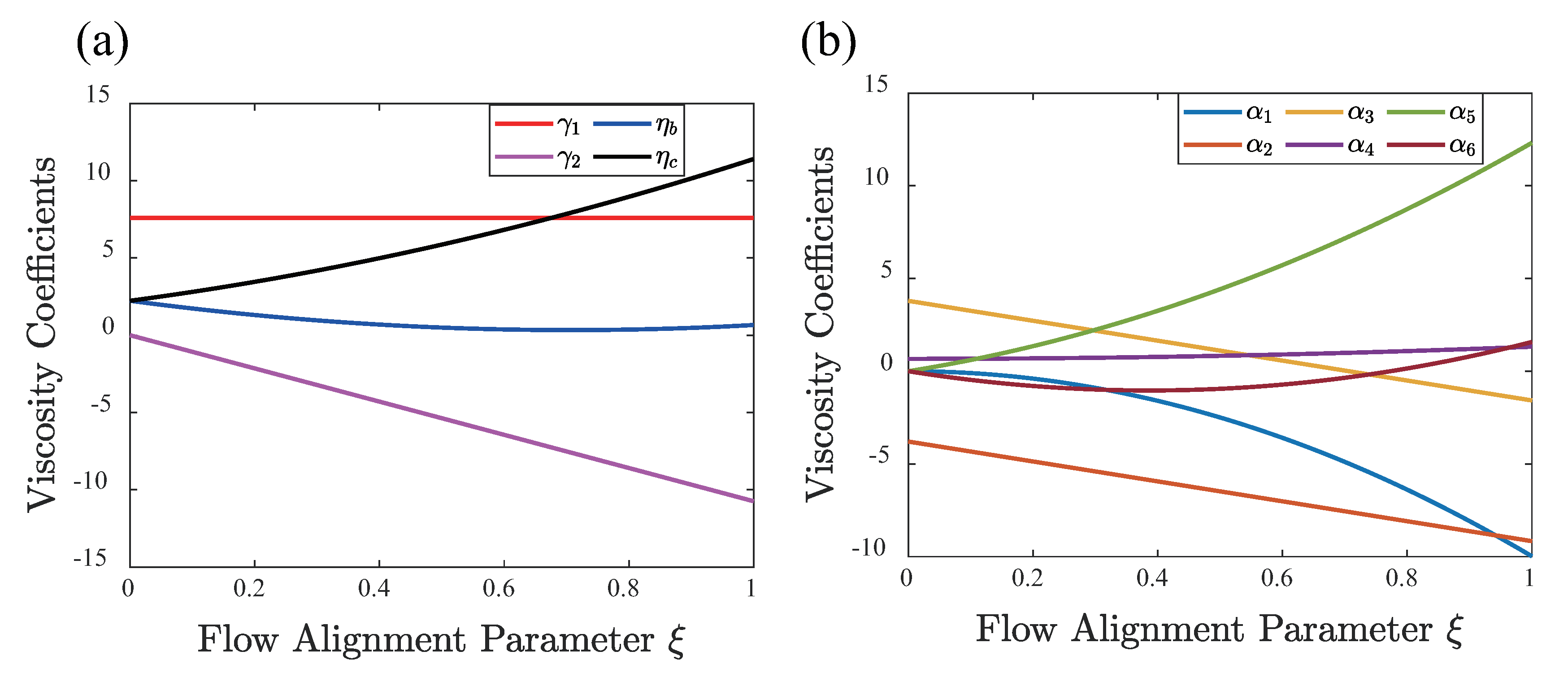
Appendix A.1. Mapping of Leslie Viscosity Coefficients

The six Leslie viscosity coefficients α i with i = 1 , 2 , . . . , 6 in LBM can be mapped according to the following [54].
α 1 = 2 3 S 0 2 ( 3 + 4 S 0 4 S 0 2 ) ξ 2 / Γ , α 2 = 1 3 S 0 ( 2 + S 0 ) ξ S 0 2 / Γ , α 3 = 1 3 S 0 ( 2 + S 0 ) ξ + S 0 2 / Γ , α 4 = 4 9 ( 1 S 0 ) 2 ξ 2 / Γ + 2 η , α 5 = 1 3 S 0 ( 4 S 0 ) ξ 2 + 1 3 S 0 ( 2 + S 0 ) ξ / Γ , α 6 = 1 3 S 0 ( 4 S 0 ) ξ 2 1 3 S 0 ( 2 + S 0 ) ξ / Γ .
Rotational viscosity reads as follows. [54]
γ 1 = α 3 α 2 = 2 S 0 2 Γ .
The above relations are used to facilitate the comparison between LBM simulation and LE theory. In Figure A1, we plotted these viscosity coefficients as functions of flow aligning parameter ξ with fixed Γ = 0.1 and S 0 0.62 .
Figure A1. Viscosity Coefficients in LBM Simulation. (a): Rotational viscosity γ 1 and Miesowicz viscosities as functions of flow aligning parameter ξ . (b): Leslie viscosity coefficients as functions of flow aligning parameter ξ . Values are reported in simulation units.
Crystals 11 01071 g0a1

Appendix A.2. Derivation of Tumbling Frequency

When the nematic LC is subjected to a simple shear flow without any elastic distortion due to anchoring, the governing equations of its director field can be simplified as follows:
γ 1 ϕ ˙ sin θ = γ ˙ α 2 cos θ cos ϕ ,
γ 1 θ ˙ = γ ˙ α 2 cos 2 θ + α 3 sin 2 θ sin ϕ ,
where γ 1 is the rotational viscosity of the LC and γ ˙ is the shear rate. By assuming flow-tumbling nematic, we chose Leslie viscosity coefficient α 2 < 0 and α 3 > 0 . Consider the director freely tumbling within the shear plane, ϕ π 2 . By integrating Equation (A4), we have the following:
0 π / 2 d θ α 2 cos 2 θ + α 3 sin 2 θ = 0 T / 4 γ ˙ γ 1 d t = γ ˙ γ 1 T 4
where T is the period of free tumbling. Solving the above integral, we arrive at Equation (9).
ω = ω tumbling = 2 π T = α 2 α 3 γ 1 γ ˙ .
Note that the angular frequency is proportional to the shear rate γ ˙ . Therefore, we report scaled angular frequency ω / γ ˙ = α 2 α 3 γ 1 in Figure 9. We compare the scaled angular frequency measured in the LBM simulation to Equation (9) and observe good agreement (Figure 9a).
We next evaluate the frequency for log-rolling mode. When the directors are close to x-direction, we can assume that θ = π 2 + θ 1 , ϕ = 0 + ϕ 1 , with θ 1 and ϕ 1 being the two small variables. By inserting the above equations into Equations (A3) and (A4) and retaining first-order terms, we have the following.
γ 1 ϕ 1 ˙ = γ ˙ α 2 θ 1 γ 1 θ 1 ˙ = γ ˙ α 3 ϕ 1
Therefore, the following is the case.
γ 1 θ 1 ¨ = γ ˙ α 3 ϕ 1 ˙ = γ ˙ 2 α 2 α 3 γ 1 θ 1 .
By solving the above second-order differential equation, we obtain the following.
θ 1 = ϵ sin ( γ ˙ γ 1 α 2 α 3 t ) ,
where ϵ is the amplitude of the unsteady dynamics. Thus, we have proved that in the log-rolling mode, the angular frequency is identical to Equation 9: ω log - rolling = ω tumbling = α 2 α 3 γ 1 γ ˙ .

References

  1. de Gennes, P.; Prost, J. The Physics of Liquid Crystals; Oxford University Press, Inc.: Oxford, UK, 1995. [Google Scholar]
  2. Kleman, M.; Laverntovich, O.D. Soft Matter Physics: An Introduction; Springer Science & Business Media: New York, NY, USA, 2007. [Google Scholar]
  3. Lin, I.H.; Miller, D.S.; Bertics, P.J.; Murphy, C.J.; De Pablo, J.J.; Abbott, N.L. Endotoxin-induced structural transformations in liquid crystalline droplets. Science 2011, 332, 1297–1300. [Google Scholar] [CrossRef] [Green Version]
  4. Sadati, M.; Apik, A.I.; Armas-Perez, J.C.; Martinez-Gonzalez, J.; Hernandez-Ortiz, J.P.; Abbott, N.L.; de Pablo, J.J. Liquid crystal enabled early stage detection of beta amyloid formation on lipid monolayers. Adv. Funct. Mater. 2015, 25, 6050–6060. [Google Scholar] [CrossRef]
  5. Muševič, I.; Škarabot, M.; Tkalec, U.; Ravnik, M.; Žumer, S. Two-Dimensional Nematic Colloidal Crystals Self-Assembled by Topological Defects. Science 2006, 313, 954–958. [Google Scholar] [CrossRef] [PubMed]
  6. Whitmer, J.K.; Wang, X.; Mondiot, F.; Miller, D.S.; Abbott, N.L.; de Pablo, J.J. Nematic-Field-Driven Positioning of Particles in Liquid Crystal Droplets. Phys. Rev. Lett. 2013, 11, 227801. [Google Scholar] [CrossRef] [Green Version]
  7. Rahimi, M.; Roberts, T.F.; Armas-Pérez, J.C.; Wang, X.; Bukusoglu, E.; Abbott, N.L.; de Pablo, J.J. Nanoparticle self-assembly at the interface of liquid crystal droplets. Proc. Natl. Acad. Sci. USA 2015, 112, 5297–5302. [Google Scholar] [CrossRef] [Green Version]
  8. Wang, X.; Miller, D.S.; Bukusoglu, E.; de Pablo, J.J.; Abbott, N.L. Topological defects in liquid crystals as templates for molecular self-assembly. Nat. Mater. 2015, 15, 106. [Google Scholar] [CrossRef] [PubMed]
  9. Wang, X.; Kim, Y.K.; Bukusoglu, E.; Zhang, B.; Miller, D.S.; Abbott, N.L. Experimental Insights into the Nanostructure of the Cores of Topological Defects in Liquid Crystals. Phys. Rev. Lett. 2016, 116, 147801. [Google Scholar] [CrossRef] [PubMed] [Green Version]
  10. Lavrentovich, O.D. Transport of particles in liquid crystals. Soft Matter 2014, 10, 1264–1283. [Google Scholar] [CrossRef] [PubMed] [Green Version]
  11. Mo, J.; Milleret, G.; Nagaraj, M. Liquid crystal nanoparticles for commercial drug delivery. Liq. Cryst. Rev. 2017, 5, 69–85. [Google Scholar] [CrossRef]
  12. Lavrentovich, O.D. Design of nematic liquid crystals to control microscale dynamics. Liq. Cryst. Rev. 2020, 8, 59–129. [Google Scholar] [CrossRef]
  13. Sengupta, A.; Tkalec, U.; Bahr, C. Nematic textures in microfluidic environment. Soft Matter 2011, 7, 6542–6549. [Google Scholar] [CrossRef]
  14. Sengupta, A.; Tkalec, U.; Ravnik, M.; Yeomans, J.M.; Bahr, C.; Herminghaus, S. Liquid crystal microfluidics for tunable flow shaping. Phys. Rev. Lett. 2013, 110, 048303. [Google Scholar] [CrossRef] [PubMed]
  15. Sengupta, A.; Herminghaus, S.; Bahr, C. Liquid crystal microfluidics: Surface, elastic and viscous interactions at microscales. Liq. Cryst. Rev. 2014, 2, 73–110. [Google Scholar] [CrossRef]
  16. Giomi, L.; Kos, Ž.; Ravnik, M.; Sengupta, A. Cross-talk between topological defects in different fields revealed by nematic microfluidics. Proc. Natl. Acad. Sci. USA 2017, 114, E5771–E5777. [Google Scholar] [CrossRef] [Green Version]
  17. Emeršič, T.; Zhang, R.; Kos, Ž.; Čopar, S.; Osterman, N.; De Pablo, J.J.; Tkalec, U. Sculpting stable structures in pure liquids. Sci. Adv. 2019, 5, eaav4283. [Google Scholar] [CrossRef] [PubMed] [Green Version]
  18. Čopar, S.; Kos, Ž.; Emeršič, T.; Tkalec, U. Microfluidic control over topological states in channel-confined nematic flows. Nat. Commun. 2020, 11, 1–10. [Google Scholar] [CrossRef]
  19. Rey, A.D. Liquid crystal models of biological materials and processes. Soft Matter 2010, 6, 3402–3429. [Google Scholar] [CrossRef]
  20. Saw, T.B.; Doostmohammadi, A.; Nier, V.; Kocgozlu, L.; Thampi, S.; Toyama, Y.; Marcq, P.; Lim, C.T.; Yeomans, J.M.; Ladoux, B. Topological defects in epithelia govern cell death and extrusion. Nature 2017, 544, 212–216. [Google Scholar] [CrossRef] [PubMed]
  21. Kawaguchi, K.; Kageyama, R.; Sano, M. Topological defects control collective dynamics in neural progenitor cell cultures. Nature 2017, 545, 327–331. [Google Scholar] [CrossRef]
  22. Marchetti, M.C.; Joanny, J.F.; Ramaswamy, S.; Liverpool, T.B.; Prost, J.; Rao, M.; Simha, R.A. Hydrodynamics of soft active matter. Rev. Mod. Phys. 2013, 85, 1143. [Google Scholar] [CrossRef] [Green Version]
  23. Doostmohammadi, A.; Ignés-Mullol, J.; Yeomans, J.M.; Sagués, F. Active nematics. Nat. Commun. 2018, 9, 3246. [Google Scholar] [CrossRef]
  24. Needleman, D.; Dogic, Z. Active matter at the interface between materials science and cell biology. Nat. Rev. Mater. 2017, 2, 1–14. [Google Scholar] [CrossRef]
  25. Zhang, R.; Mozaffari, A.; de Pablo, J.J. Autonomous materials systems from active liquid crystals. Nat. Rev. Mater. 2021, 6, 437–453. [Google Scholar] [CrossRef]
  26. Sanchez, T.; Chen, D.T.; DeCamp, S.J.; Heymann, M.; Dogic, Z. Spontaneous motion in hierarchically assembled active matter. Nature 2012, 491, 431–434. [Google Scholar] [CrossRef] [Green Version]
  27. Kumar, N.; Zhang, R.; de Pablo, J.J.; Gardel, M.L. Tunable structure and dynamics of active liquid crystals. Sci. Adv. 2018, 4, eaat7779. [Google Scholar] [CrossRef] [Green Version]
  28. Li, H.; Shi, X.; Huang, M.; Chen, X.; Xiao, M.; Liu, C.; Chaté, H.; Zhang, H. Data-driven quantitative modeling of bacterial active nematics. Proc. Natl. Acad. Sci. USA 2019, 116, 777–785. [Google Scholar] [CrossRef] [Green Version]
  29. Zhou, S.; Sokolov, A.; Lavrentovich, O.D.; Aranson, I.S. Living liquid crystals. Proc. Natl. Acad. Sci. USA 2014, 111, 1265–1270. [Google Scholar] [CrossRef] [Green Version]
  30. Genkin, M.M.; Sokolov, A.; Lavrentovich, O.D.; Aranson, I.S. Topological defects in a living nematic ensnare swimming bacteria. Phys. Rev. X 2017, 7, 011029. [Google Scholar] [CrossRef] [Green Version]
  31. Sokolov, A.; Mozaffari, A.; Zhang, R.; De Pablo, J.J.; Snezhko, A. Emergence of radial tree of bend stripes in active nematics. Phys. Rev. X 2019, 9, 031014. [Google Scholar] [CrossRef] [Green Version]
  32. Turiv, T.; Koizumi, R.; Thijssen, K.; Genkin, M.M.; Yu, H.; Peng, C.; Wei, Q.H.; Yeomans, J.M.; Aranson, I.S.; Doostmohammadi, A.; et al. Polar jets of swimming bacteria condensed by a patterned liquid crystal. Nat. Phys. 2020, 16, 481–487. [Google Scholar] [CrossRef] [Green Version]
  33. Duclos, G.; Adkins, R.; Banerjee, D.; Peterson, M.S.; Varghese, M.; Kolvin, I.; Baskaran, A.; Pelcovits, R.A.; Powers, T.R.; Baskaran, A.; et al. Topological structure and dynamics of three-dimensional active nematics. Science 2020, 367, 1120–1124. [Google Scholar] [CrossRef] [Green Version]
  34. Giomi, L.; Liverpool, T.B.; Marchetti, M.C. Sheared active fluids: Thickening, thinning, and vanishing viscosity. Phys. Rev. E 2010, 81, 051908. [Google Scholar] [CrossRef] [PubMed] [Green Version]
  35. Guillamat, P.; Ignés-Mullol, J.; Shankar, S.; Marchetti, M.C.; Sagués, F. Probing the shear viscosity of an active nematic film. Phys. Rev. E 2016, 94, 060602. [Google Scholar] [CrossRef] [Green Version]
  36. Lydon, J. Chromonic liquid crystalline phases. Liq. Cryst. 2011, 38, 1663–1681. [Google Scholar] [CrossRef]
  37. Zimmermann, N.; Jünnemann-Held, G.; Collings, P.J.; Kitzerow, H.S. Self-organized assemblies of colloidal particles obtained from an aligned chromonic liquid crystal dispersion. Soft Matter 2015, 11, 1547–1553. [Google Scholar] [CrossRef] [Green Version]
  38. Park, H.S.; Kang, S.W.; Tortora, L.; Nastishin, Y.; Finotello, D.; Kumar, S.; Lavrentovich, O.D. Self-assembly of lyotropic chromonic liquid crystal Sunset Yellow and effects of ionic additives. J. Phys. Chem. B 2008, 112, 16307–16319. [Google Scholar] [CrossRef]
  39. Zhou, S.; Neupane, K.; Nastishin, Y.A.; Baldwin, A.R.; Shiyanovskii, S.V.; Lavrentovich, O.D.; Sprunt, S. Elasticity, viscosity, and orientational fluctuations of a lyotropic chromonic nematic liquid crystal disodium cromoglycate. Soft Matter 2014, 10, 6571–6581. [Google Scholar] [CrossRef]
  40. Davidson, Z.S.; Kang, L.; Jeong, J.; Still, T.; Collings, P.J.; Lubensky, T.C.; Yodh, A. Chiral structures and defects of lyotropic chromonic liquid crystals induced by saddle-splay elasticity. Phys. Rev. E 2015, 91, 050501. [Google Scholar] [CrossRef] [Green Version]
  41. Nayani, K.; Chang, R.; Fu, J.; Ellis, P.W.; Fernandez-Nieves, A.; Park, J.O.; Srinivasarao, M. Spontaneous emergence of chirality in achiral lyotropic chromonic liquid crystals confined to cylinders. Nat. Commun. 2015, 6, 1–7. [Google Scholar] [CrossRef]
  42. Jeong, J.; Davidson, Z.S.; Collings, P.J.; Lubensky, T.C.; Yodh, A. Chiral symmetry breaking and surface faceting in chromonic liquid crystal droplets with giant elastic anisotropy. Proc. Natl. Acad. Sci. USA 2014, 111, 1742–1747. [Google Scholar] [CrossRef] [PubMed] [Green Version]
  43. Park, G.; Čopar, S.; Suh, A.; Yang, M.; Tkalec, U.; Yoon, D.K. Periodic Arrays of Chiral Domains Generated from the Self-Assembly of Micropatterned Achiral Lyotropic Chromonic Liquid Crystal. ACS Cent. Sci. 2020, 6, 1964–1970. [Google Scholar] [CrossRef]
  44. Lavrentovich, M.; Sergan, T.; Kelly, J. Planar and twisted lyotropic chromonic liquid crystal cells as optical compensators for twisted nematic displays. Liq. Cryst. 2003, 30, 851–859. [Google Scholar] [CrossRef]
  45. Shiyanovskii, S.V.; Lavrentovich, O.D.; Schneider, T.; Ishikawa, T.; Smalyukh, I.I.; Woolverton, C.J.; Niehaus, G.D.; Doane, K.J. Lyotropic chromonic liquid crystals for biological sensing applications. Mol. Cryst. Liq. Cryst. 2005, 434, 259–587. [Google Scholar] [CrossRef]
  46. Sharma, A.; Ong, I.L.H.; Sengupta, A. Time dependent lyotropic chromonic textures in microfluidic confinements. Crystals 2021, 11, 35. [Google Scholar] [CrossRef]
  47. Peng, C.; Turiv, T.; Guo, Y.; Wei, Q.H.; Lavrentovich, O.D. Command of active matter by topological defects and patterns. Science 2016, 354, 882–885. [Google Scholar] [CrossRef] [Green Version]
  48. Baza, H.; Turiv, T.; Li, B.X.; Li, R.; Yavitt, B.M.; Fukuto, M.; Lavrentovich, O.D. Shear-induced polydomain structures of nematic lyotropic chromonic liquid crystal disodium cromoglycate. Soft Matter 2020, 16, 8565–8576. [Google Scholar] [CrossRef]
  49. Zhang, Q.; Zhang, R.; Ge, B.; Yaqoob, Z.; So, P.T.C.; Bischofberger, I. Structures and topological defects in pressure-driven lyotropic chromonic liquid crystals. Proc. Natl. Acad. Sci. USA 2021, 118, e2108361118. [Google Scholar] [CrossRef]
  50. Thampi, S.P.; Golestanian, R.; Yeomans, J.M. Driven active and passive nematics. Mol. Phys. 2015, 113, 2656–2665. [Google Scholar] [CrossRef] [Green Version]
  51. Thijssen, K.; Metselaar, L.; Yeomans, J.M.; Doostmohammadi, A. Active nematics with anisotropic friction: The decisive role of the flow aligning parameter. Soft Matter 2020, 16, 2065–2074. [Google Scholar] [CrossRef] [Green Version]
  52. Chandragiri, S.; Doostmohammadi, A.; Yeomans, J.M.; Thampi, S.P. Flow states and transitions of an active nematic in a three-dimensional channel. Phys. Rev. Lett. 2020, 125, 148002. [Google Scholar] [PubMed]
  53. Pieranski, P.; Guyon, E.; Pikin, S. Nouvelles instabilités de cisaillement dans les nématiques. J. Phys. Colloq. 1976, 37, C1-3. [Google Scholar] [CrossRef]
  54. Denniston, C.; Orlandini, E.; Yeomans, J.M. Lattice Boltzmann simulations of liquid crystal hydrodynamics. Phys. Rev. E 2001, 63, 056702. [Google Scholar] [CrossRef] [PubMed] [Green Version]
  55. Beris, A.N.; Edwards, B.J. Thermodynamics of Flowing Systems: With Internal Microstructure; Number 36, Oxford University Press on Demand: Oxford, UK, 1994. [Google Scholar]
  56. Ravnik, M.; Žumer, S. Landau–de Gennes modelling of nematic liquid crystal colloids. Liq. Cryst. 2009, 36, 1201–1214. [Google Scholar] [CrossRef]
  57. Denniston, C.; Marenduzzo, D.; Orlandini, E.; Yeomans, J. Lattice Boltzmann algorithm for three–dimensional liquid–crystal hydrodynamics. Philos. Trans. R. Soc. London. Ser. Math. Phys. Eng. Sci. 2004, 362, 1745–1754. [Google Scholar] [CrossRef]
  58. Zhang, R.; Roberts, T.; Aranson, I.S.; De Pablo, J.J. Lattice Boltzmann simulation of asymmetric flow in nematic liquid crystals with finite anchoring. J. Chem. Phys. 2016, 144, 084905. [Google Scholar] [CrossRef]
  59. Giomi, L.; Bowick, M.J.; Ma, X.; Marchetti, M.C. Defect annihilation and proliferation in active nematics. Phys. Rev. Lett. 2013, 110, 228101. [Google Scholar] [CrossRef]
  60. Marenduzzo, D.; Orlandini, E.; Cates, M.; Yeomans, J. Steady-state hydrodynamic instabilities of active liquid crystals: Hybrid lattice Boltzmann simulations. Phys. Rev. E 2007, 76, 031921. [Google Scholar] [CrossRef] [PubMed] [Green Version]
  61. Ravnik, M.; Yeomans, J.M. Confined active nematic flow in cylindrical capillaries. Physical review letters 2013, 110, 026001. [Google Scholar] [CrossRef]
  62. Green, R.; Toner, J.; Vitelli, V. Geometry of thresholdless active flow in nematic microfluidics. Phys. Rev. Fluids 2017, 2, 104201. [Google Scholar] [CrossRef]
  63. Zhou, S.; Nastishin, Y.A.; Omelchenko, M.M.; Tortora, L.; Nazarenko, V.G.; Boiko, O.P.; Ostapenko, T.; Hu, T.; Almasan, C.C.; Sprunt, S.N.; et al. Elasticity of lyotropic chromonic liquid crystals probed by director reorientation in a magnetic field. Phys. Rev. Lett. 2012, 109, 037801. [Google Scholar] [CrossRef] [PubMed] [Green Version]
  64. Strübing, T.; Khosravanizadeh, A.; Vilfan, A.; Bodenschatz, E.; Golestanian, R.; Guido, I. Wrinkling instability in 3D active nematics. Nano Lett. 2020, 20, 6281–6288. [Google Scholar] [CrossRef] [PubMed]
  65. Nejad, M.R.; Yeomans, J.M. Extensile stress promotes out-of-plane flows in active layers. arXiv 2021, arXiv:2105.10812. [Google Scholar]
  66. Jewell, S.A.; Cornford, S.L.; Yang, F.; Cann, P.; Sambles, J.R. Flow-driven transition and associated velocity profiles in a nematic liquid-crystal cell. Phys. Rev. E 2009, 80, 041706. [Google Scholar] [CrossRef] [PubMed]
  67. Batista, V.M.; Blow, M.L.; da Gama, M.M.T. The effect of anchoring on the nematic flow in channels. Soft Matter 2015, 11, 4674–4685. [Google Scholar] [CrossRef] [PubMed] [Green Version]
Figure 1. Simulation setup. Two walls are in z-direction separated by a distance of L z . Easy axis is in the y-direction. Couette flow is imposed by moving top and bottom wall in y-direction with speed u 0 and u 0 , respectively. Poiseuille flow is imposed by applying a pressure gradient G along y-direction. Director field n is represented by a polar angle θ and an azimuthal angle ϕ .
Crystals 11 01071 g001
Figure 2. Steady -state Couette flow of a flow-aligning nematic. Infinite nondegenerate anchoring condition for both walls is considered. Polar angle θ (a) and y-velocity u y (b) for passive nematic (Er = 10, 50 and 100). Polar angle θ (c) and y-velocity u y (d) for active nematic with activity α / α 0 = 5.1 (Er = 10, 20, 30 and 40). In infinite planar anchoring with y-axis, the easy axis is considered for (ad). Results from Leslie–Ericksen theory and lattice Boltzmann method are represented by lines and triangles, respectively.
Crystals 11 01071 g002
Figure 3. Spontaneous flow of flow-aligning active nematic in a hybrid cell. (a) The director field of LC under different activity levels. Planar anchoring is imposed to bottom wall ( θ = 90°), and homeotropic anchoring is imposed to the top wall (0°). The color of the line represents different activity levels. The inset in (a) illustrates the director field in the hybrid cell; (b) y-velocity profile in the channel; (c) the effective shear viscosity in the channel; (d) net flow rate in y direction.
Crystals 11 01071 g003
Figure 4. Tumbling active nematic LC flow in a hybrid cell at low to intermediate activity. Top and bottom wall have planar and homeotropic finite nondegenrate anchoring condition, respectively. (a,b) Director field (polar angle and azimuthal angle) at different activity levels. The inset in (a) is the scalar order parameter profile. The inset in (b) illustrates director being at log-rolling state. The (c) y-velocity profile. The (d) x-velocity (transverse flow). Line color represents different activity levels.
Crystals 11 01071 g004
Figure 5. Evolution dynamics of tumbling active nematic flow in a hybrid cell at high activity. Top wall and bottom walls are planar and finite homeotropic anchoring, respectively, with W = 1 in simulation units and activity α / α 0 = 20.4 . (ac) Time sequence of the director field. (a) Sequential snapshots of the director field colored by scalar order parameter. Time evolution of polar angle θ (b), azimuthal angle ϕ (c), easy-axis flow profile u y (d) and transverse flow profile u x (e). Velocity is reported in simulation units. Color in (be) represents different times (legend in (c)).
Crystals 11 01071 g005
Figure 6. Spontaneous net flows of tumbling active nematic in a hybrid cell. Director field in terms of polar angle θ (a) and azimuthal angle ϕ (b) under different activity levels ranging from 2.6 to 35.7 (color from blue to red). Easy-axis flow profile u y (c) and the corresponding flow rate q y (blue circles in (e)). Transverse flow profile u x (d) and the corresponding flow rate q x (blue circles in (f)). Red triangles in (e) and (f) represent total flow rate q and flow rate ratio indicator ψ = arctan ( q x / q y ) , respectively.
Crystals 11 01071 g006
Figure 7. Activity suppressing and promoting Poiseuille flow in a nematic planar cell. (a) The flow rate (q) of an active nematic with different flow-alignment parameters ξ under a fixed pressure gradient G = 2 × 10 5 corresponding to Er = 35. (b) Effective viscosities in the cell with zero activity level. (c) Director field in the cell under pressure driven flow with zero activity level. (d) Active force (shown in Equation (8)) distribution under pressure-driven flow with activity α / α 0 = 5.1 . Black triangles, blue squares and red dots represent ξ = 0.6 , 0.7 and 0.8 , respectively.
Crystals 11 01071 g007
Figure 8. “Bowser-dowser” transition of an active nematic in a homeotropic cell. (a) Nematic LC under Poiseuille flow has two steady-states. Black line shows the director field of “bowser” state, and red line shows the director field of “dowser” state. (b) State diagram in terms of pressure gradient G and activity α / α 0 . Black solid line, blue dashed line and red dashed line represent ξ = 0.6, 0.7 and 0.8, respectively. Bottom left region is the “bowser” state, and top right region is the “dowser” state. The insets of different region show the schematic director field of the “bowser” and “dowser” state. Ericksen number is between Er = 17.5 ( G = 10 5 ) and Er = 63 ( G = 3.6 × 10 5 ).
Crystals 11 01071 g008
Figure 9. Tumbling dynamics frequency for an active nematic under Couette flow. (a) Scaled angular frequency ω / γ ˙ for free tumbling, passive nematic as a function of shear rate γ ˙ . Blue dots are from LBM simulation, and the dashed line is the theoretical value adopted from Equation (9). (b) Scaled angular frequency ω / γ ˙ for tumbling active nematic under Couette flow with finite nondegenerate planar anchoring as a function of scaled activity α / α 0 . Black dashed line is the theoretical value for passive nematics. Blue dots and red circles represent shear rate γ ˙ = 4 × 10 4 (Er = 100) and γ ˙ = 6 × 10 4 (Er = 50) in simulation units, respectively. (c) State diagram of tumbling nematics in terms of Ericksen number Er and activity-related dimensionless number α L z / K 1 γ 1 γ ˙ .
Crystals 11 01071 g009
Figure 10. Spatiotemporal pattern of tumbling active nematics. Snapshots of tumbling nematic under Couette flow at α / α 0 = 2.6 (a) and 7.1 (b). Shear rate is γ ˙ = 4 × 10 4 for both scenarios. Color represents out-of-plane director | n x | . Ticks and dots in (a) and (b) represent the projection of the directors in the shear plane. (c) θ - ϕ trajectory at black square area in (a). (dg) and (k,l): θ - ϕ trajectory in corresponding locations marked in (b). Red arrows indicate time arrow. (h) Polar angle profile in (a). Profiles of polar angle (i) and azimuthal angle (j) in (b).
Crystals 11 01071 g010
Publisher’s Note: MDPI stays neutral with regard to jurisdictional claims in published maps and institutional affiliations.

